Effect of hydrogen bond cooperativity on the behavior of water

Abstract

Four scenarios have been proposed for the low–temperature phase behavior of liquid water, each predicting different thermodynamics. The physical mechanism which leads to each is debated. Moreover, it is still unclear which of the scenarios best describes water, as there is no definitive experimental test. Here we address both open issues within the framework of a microscopic cell model by performing a study combining mean field calculations and Monte Carlo simulations. We show that a common physical mechanism underlies each of the four scenarios, and that two key physical quantities determine which of the four scenarios describes water: (i) the strength of the directional component of the hydrogen bond and (ii) the strength of the cooperative component of the hydrogen bond. The four scenarios may be mapped in the space of these two quantities. We argue that our conclusions are model-independent. Using estimates from experimental data for H bond properties the model predicts that the low-temperature phase diagram of water exhibits a liquid–liquid critical point at positive pressure.

Water’s phase diagram is rich and complex: more than sixteen crystalline phases Zheligovskaya , and two or more glasses Debenedetti-JPCM03 ; loerting ; gruner have been reported. The liquid state also displays interesting behavior, such as the density maximum for 1 atm at $4^{\circ}$C. The volume fluctuations $\left<(\delta V)^{2}\right>$, entropy fluctuations $\left<(\delta S)^{2}\right>$, and cross-fluctuations between volume and entropy $\left<\delta V\delta S\right>$, proportional to the magnitude of isothermal compressibility $K_{T}$, isobaric specific heat $C_{P}$, and isobaric thermal expansivity $\alpha_{P}$, respectively, show anomalous increases in magnitude upon cooling angelldiv . Further, these quantities display an apparent divergence for 1 atm at $-45^{\circ}$C angelldiv , hinting at interesting phase behavior in the supercooled region.

Microscopically, water’s anomalous liquid behavior is understood as resulting from the tendency of neighboring molecules to form hydrogen (H) bonds upon cooling, with a decrease of local potential energy, decrease of local entropy, and increase of local volume due to the formation of local open structures of bonded molecules. Different models include these H-bond features, but depending on the assumptions and approximations of each model, different conclusions are obtained for the low–T phase behavior. The relevant region of the bulk liquid state cannot be probed experimentally, and none of the theories tested, because crystallization of bulk water is unavoidable below the homogeneous nucleation temperature $T_{H}$ ($-38^{\circ}$C at 1 atm).

I Four scenarios for supercooled water

Due to the difficulty of obtaining experimental evidence, theoretical and numerical analyses are useful. Four separate scenarios for the pressure–temperature ($P-T$) phase diagram have been proposed:

(I) The stability limit (SL) scenario Speedy82 hypothesizes that the superheated liquid-gas spinodal at negative pressure re-enters the positive $P$ region below $T_{H}(P)$. In this view, the liquid state is delimited by a single continuous locus, $P_{s}(T)$, bounding the superheated, stretched and supercooled states. There is no reference to the phase into which the liquid transforms when $P\to P_{s}(T)$. As the spinodal is approached, $K_{T}$, $C_{P}$, and $\alpha_{P}\to\infty$. A thermodynamic consequence of the SL scenario is that the intersection of the retracing spinodal with the liquid–vapor coexistence line must be a critical point Debenedetti-JPCM03 . The presence of a such a critical point in the liquid–vapor transition, although possible, is not confirmed by any experiment. This fact poses a serious challenge to the SL scenario.

(II) The liquid–liquid critical point (LLCP) scenario pses hypothesizes a first–order phase transition line between two liquids — a low density liquid (LDL), and a high density liquid (HDL) — which terminates at a liquid–liquid critical point $C^{\prime}$. HDL is a dense liquid with a highly disordered structure, whereas LDL has a lower density and locally tetrahedral order. The experimentally observable high density amorphous (HDA) and low density amorphous (LDA) solids correspond, in this scenario, to a structurally arrested state of HDL and LDL respectively StarrPRE99 ; BellissentJCP95 . Starting from $C^{\prime}$, the locus of maxima of the correlation length $\xi$ (the Widom line) projects into the one–phase region Xu-PNAS05 . Asymptotically close to the critical point, response functions can be expressed in terms of $\xi$, hence, these too will show maxima, e.g., as a function of $T$ upon isobaric cooling. These maxima will diverge upon approaching $C^{\prime}$. Furthermore, for $P>P_{C^{\prime}}$, the pressure of $C^{\prime}$, the response functions will diverge by approaching the spinodal converging to $C^{\prime}$. Specific models suggest psgsa ; pses that $P_{C^{\prime}}>0$, but the possibility $P_{C^{\prime}}<0$ has also been proposed t .

(III) The singularity–free (SF) scenario sdss hypothesizes that the low-$T$ anticorrelation between volume and entropy is sufficient to cause the response functions to increase upon cooling and display maxima at non–zero $T$, without reference to any singular behavior. Specifically, Sastry et al. sdss consider the temperature of maximum density (TMD) line, where the density has a maximum as a function of temperature, and prove a general thermodynamic theorem establishing the proportionality between the slope of the TMD, $(\partial P/\partial T)_{\mathrm{TMD}}$, and the temperature derivative of $K_{T}$. Thus, since the TMD has negative slope in water, it follows that $(\partial P/\partial T)_{\mathrm{TMD}}<0$, and therefore $K_{T}$ must increase upon cooling, whether there exists a singularity or not.

(IV) The critical–point free (CPF) scenario a hypothesizes an order–disorder transition, with possibly a weak first–order transition character, separating two liquid phases and extending to $P<0$ down to the superheated limit of stability of liquid water. This scenario effectively predicts a continuous locus of stability limit spanning the superheated, stretched and supercooled state, because the spinodal associated with the first–order transition will intersect the liquid–gas spinodal at negative pressure. No critical point is present in this scenario.

These four scenarios predict fundamentally different behavior, though each has been rationalized as a consequence of the same microscopic interaction: the H bond. A question that naturally arises is whether the macroscopic thermodynamic descriptions are in fact connected in some way. Previous works have attempted to uncover relations between several of the scenarios, for example between (I) and (II) psgsa ; bds or (II) and (III) tdst ; tanaka2000 . Here we offer a relation linking all four scenarios showing that (a) all four can be included in one general scheme, (b) the balance between the energies of two components of the H bond interaction determines which scenario is valid. Morevover, we argue that current values for these energies support the LLCP scenario.

II Cooperative cell model of water

We analyze a microscopic model fs of water in which the fluid is divided into $N$ cells with nearest neighbor (n.n.) interactions. The division is such that each cell is in contact with four n.n., mimicking the first shell of liquid water. The case of a shared H bond, due to more than four molecules in the first shell, is assimilated with the case in which a H bond is broken, since the interaction energy of a shared bond is less than half the energy of a single H bond sfs ; ek .

The goal of the model is to represent, microscopically, the essential features of the interaction among water molecules, while being able to qualitatively understand the importance of each of these features. To this end the interaction among cells is separated into four distinct components.

The first component of the interaction is due to the short–range repulsion of the electron clouds. This is incorporated into the model by assigning to each cell $i\in[1,N]$ (a) a volume $v_{i}\geq v_{0}$, where $v_{0}$ is the exclusion volume per molecule, and (b) a maximum of one molecule.

The second component includes all the isotropic long–range attractive interactions, such as the instantaneous induced dipole-dipole (London) interactions between the electron clouds of different molecules or the isotropic part of the hydrogen bond hbond . We refer to this component as the van der Waals attractive interaction, keeping in mind, however, that this component includes not only the (weak) London dispersion interaction, but also the (stronger) isotropic interaction of the hydrogen bond. The overall sum of the isotropic —attractive and repulsive— interactions can be represented in different ways. The one we adopt in a mean field (MF) treatment is

$$\mathscr{H}_{\rm o}\equiv-\epsilon\sum_{\langle i,j\rangle}n_{i}n_{j},$$ (1)

where if $v_{0}/v_{i}\leq 0.5$ we set the index $n_{i}=0$, and if $0.5<v_{0}/v_{i}\leq 1$ we set $n_{i}=1$, hence $n_{i}=0$ if the density in the cell is gas-like, and $n_{i}=1$ if the density in the cell is liquid-like; $\epsilon>0$ is the characteristic energy of the attraction and the sum is over all n.n. pairs $\langle i,j\rangle$.

The characteristic feature of H₂O is its ability to form H bonds between neighboring molecules. This interaction has a strong directional component due to the dipole-dipole interaction between the highly concentrated positive charge on each H and each of the two excess negative charges concentrated on the O of another water molecule. Accordingly, the third component incorporated here is this orientational–dependent interaction, which includes the covalent component of the bond hbond0 . To account for the orientational degrees of freedom of each water molecule, we assign to each cell $i$ four bond variables $\sigma_{ij}=1,...,q$ (one for each n.n. cell $j$), representing the orientation of molecule $i$ with respect to molecule $j$. We choose the parameter $q$ by selecting 30^o as the maximum deviation from a linear bond, i.e. $q\equiv 180^{o}/30^{o}=6$, hence every molecule has $q^{4}=6^{4}\equiv 1296$ possible orientations. (The effect of choosing a different value for $q$ has been analyzed in fs-JPCM07 .) We say that a bond is formed between cells $i$ and $j$ if $\sigma_{ij}=\sigma_{ji}$.

Experiments show that formation of the H bonds leads to an open —locally tetrahedral— structure that induces an increase of volume per molecule Debenedetti-JPCM03 ; soperricci . This effect is incorporated in the model by considering the total volume to be given as

$$V\equiv Nv_{0}+N_{\rm HB}v_{\rm HB},$$ (2)

where

$$N_{\rm HB}\equiv\sum_{\langle i,j\rangle}n_{i}n_{j}\delta_{\sigma_{ij},\sigma_{ji}}$$ (3)

is the total number of H bonds, $\delta_{a,b}=1$ if $a=b$, $\delta_{a,b}=0$ if $a\neq b$, and $v_{\rm HB}$ is the volume increase per H bond sdss . Bond formation also leads to a decrease in the local potential energy, hence we add to the Hamiltonian in Eq. (1) the term

$$\mathscr{H}_{\rm HB}\equiv-JN_{\rm HB},$$ (4)

where $J>0$ is the characteristic energy of the directional component of the H bond.

Another key experimental fact is that at low $T$ the O–O–O angle distribution in water becomes sharper around the tetrahedral value ricci , suggesting an interaction that induces a cooperative behavior among bonds. For water, four–body and higher order interactions seem to be negligible with respect to the three–body term Pedulla-JCP96 ; Skinner-JPCB08 . Hence, the fourth component to the interaction potential is the many–body effect due to H bonds hbond1 ; hbond2 ; hbcoop , which minimizes the energy when the H bonds of nearby molecules assume a tetrahedral orientation. This is accomplished by further adding to the Hamiltonian in Eqs. (1) and (4) the term

$$\mathscr{H}_{\rm coop}=-J_{\sigma}\sum_{i}n_{i}\sum_{(k,\ell)_{i}}\delta_{\sigma_{ik},\sigma_{i\ell}},$$ (5)

where $J_{\sigma}>0$ is the characteristic energy of the cooperative component of the H bond, and $(k,\ell)_{i}$ indicates one of the six different pairs of the four bond variables of molecule $i$. This interaction introduces a cooperative behavior among bonds, which may be fine tuned by changing $J_{\sigma}$. Choosing $J_{\sigma}=0$ leads to H bonds which form independent of neighboring bonds sdss , while $J_{\sigma}\rightarrow\infty$ leads to fully dependent bonds sss . The total Hamiltonian is now given by

$$\mathscr{H}=\mathscr{H}_{\rm o}+\mathscr{H}_{\rm HB}+\mathscr{H}_{\rm coop}.$$ (6)

This model is studied using both MF analysis and Monte Carlo (MC) simulations fms ; kfs-PRL08 ; fs-JPCM07 ; fs-PhysA02 ; kfs-JPCM08 . Details of the MF and MC techniques are available elsewhere fs-JPCM07 ; mazza . In the following we adopt $\tilde{J}\equiv J/\epsilon$, $\tilde{J_{\sigma}}\equiv J_{\sigma}/\epsilon$ and $v_{\rm HB}=2v_{0}$.

III Mean-field results

Three qualitatively different phase diagrams are found, dependent on the strengths of the H bond energy parameters, $\tilde{J}$ and $\tilde{J_{\sigma}}$ (Fig. 1).

When $\tilde{J_{\sigma}}=0$ the model coincides with that proposed in sdss , which gives rise to the SF scenario (Fig. 1a). For $0<\tilde{J_{\sigma}}\leq\tilde{J}/2$ the model displays a liquid–liquid transition ending in a LLCP at $P_{C^{\prime}}\geq 0$ (Fig. 1b) fms . For $\tilde{J}/2<\tilde{J_{\sigma}}/<a+b\tilde{J}$, where $a=0.30\pm 001$ and $b=0.36\pm 0.01$ are fitting parameters, a LLCP occurs at $P_{C^{\prime}}<0$ (Fig. 1c). For $\tilde{J_{\sigma}}\geq a+b\tilde{J}$, a liquid-liquid transition with no critical point is found, consistent with the CPF scenario (Fig. 1d). In Fig. 2 we summarize these results in the $\tilde{J}$ vs. $\tilde{J_{\sigma}}$ parameter space.

III.1 Limiting behavior between the four cases

In the following we discuss how, by tuning $\tilde{J}$ and $\tilde{J_{\sigma}}$, we can pass from one scenario to another in a continuous way.

(i) By beginning with the LLCP scenario, and studying the limit $\tilde{J_{\sigma}}\rightarrow 0$, we find $T_{C^{\prime}}\rightarrow 0$. Moreover, we find that $K_{T}$ and $\alpha_{P}$ diverge as $|T-T_{C^{\prime}}|^{-1}$ for any value of $J_{\sigma}$, including $J_{\sigma}\rightarrow 0$ and $T_{C^{\prime}}\rightarrow 0$. Further, we find for the entropy $S$ that, for any value of $J_{\sigma}$, $(\partial S/\partial T)_{P}\propto|T-T_{C^{\prime}}|^{-1}$. Hence $C_{P}\equiv T(\partial S/\partial T)_{P}$ diverges as $|T-T_{C^{\prime}}|^{-1}$ when $T_{C^{\prime}}>0$. When $T_{C^{\prime}}=0$ ($\tilde{J_{\sigma}}=0$), $C_{P}$ is constant, as in the SF scenario rebelo . Therefore, the SF scenario coincides with the LLCP scenario in the limiting case of $T_{C^{\prime}}\rightarrow 0$, for $\tilde{J_{\sigma}}\rightarrow 0$ (Fig. 1a).

(ii) Again, beginning with the LLCP scenario, and increasing $\tilde{J_{\sigma}}$ while keeping other parameters constant, we observe that $C^{\prime}$ moves to larger $T$ and lower $P$, with $P_{C^{\prime}}<0$ for $\tilde{J_{\sigma}}\geq\tilde{J}/2$ (Fig.1c).

(iii) With further increase of $\tilde{J_{\sigma}}$, $C^{\prime}$ approaches, and eventually reaches, the liquid–gas spinodal. For larger values of $\tilde{J_{\sigma}}$ only the liquid–liquid transition remains, which is precisely the CPF scenario a (Fig. 1d). Hence the CPF scenario differs from the LLCP scenario only in that $C^{\prime}$ is now inaccessible, lying beyond the region of liquid states. The same result may be obtained by decreasing $\tilde{J}$, while fixing $\tilde{J_{\sigma}}$ and other parameters. Here a decrease of $J$ moves $C^{\prime}$ to lower pressure, i.e. towards the liquid spinodal, while the entire liquid-liquid phenomena moves to succesively lower temperature. In all cases, the location of $C^{\prime}$ varies continuously with variation of $\tilde{J}$ and $\tilde{J_{\sigma}}$.

(iv) In the case of the CPF scenario, we find that the superheated liquid-gas spinodal merges with the supercooled liquid-liquid spinodal, as in Ref. psgsa . This gives rise to a liquid spinodal which retraces in the $P$–$T$ plane. This feature resembles the main characteristic of the SL scenario, where the high-$T$ liquid has a limit of stability at $P<0$ that retraces toward $P>0$ at low $T$. Here this retracing locus is formed by two spinodal lines, with different signs of the slope, that merge at $P<0$. Therefore, in the framework of the present model, the CPF scenario and the SL scenario coincide, corresponding to the case in which the cooperative behavior is very strong.

III.2 Linearity of the lines separating one scenario from another in $\tilde{J}$–$\tilde{J_{\sigma}}$ plane

For the cell model, we can derive

$$T_{C^{\prime}}=\tilde{J}_{\sigma}/\alpha+\mathscr{O}(\tilde{J}_{\sigma}^{2})$$ (7)

and

$$P_{C^{\prime}}=(\tilde{J}^{*}/v_{\rm HB})+\beta T_{C^{\prime}}+\mathscr{O}(T_{C^{\prime}}^{2}).$$ (8)

Here $\alpha>0$ and $\beta<0$ are constants and, in the MF context, $\tilde{J}^{*}\equiv\tilde{J}+3\tilde{J}_{\sigma}$. Symbols $\mathscr{O}(X^{2})$, where $X$ is $\tilde{J}_{\sigma}$ or $T_{C^{\prime}}$, represent terms of order $X^{2}$ or higher, that are negligible when $X\ll 1$. Our MF results confirm the relations in Eq. (7) and (8), with $\alpha\simeq 0.74k_{B}/\epsilon$ and $\beta\simeq-7.4k_{B}/v_{0}$, with negligible $\mathscr{O}(X^{2})$ terms.

Therefore, we can rewrite the above relations as $\tilde{J}-P_{C^{\prime}}v_{\rm HB}/\epsilon=-(3+\beta v_{\rm HB}/\alpha)\tilde{J}_{\sigma}\equiv 2\tilde{J}_{\sigma}$, when $v_{\rm HB}=2v_{0}$. As a consequence, for the case $P_{C^{\prime}}=0$, we find $\tilde{J}_{\sigma}=\tilde{J}/2$, which is exactly what we find numerically in Fig. 2 along the line separating the LLCP scenario with $P_{C^{\prime}}>0$ (valid for $\tilde{J}_{\sigma}<\tilde{J}/2$) and the LLCP scenario with $P_{C^{\prime}}<0$ (valid for $\tilde{J}_{\sigma}>\tilde{J}/2$).

It is possible to show that Eq. (8) can be generalized to $P_{LL}=(\tilde{J}^{*}/v_{\rm HB})+\beta T_{LL}+\mathscr{O}(T_{LL}^{2})$, where $T_{LL}$ and $P_{LL}$ are the $T$ and $P$ along the liquid–liquid transition line. Our MF results are in good agreement with this prediction.

We can estimate the equation of the line separating the LLCP scenario with $P_{C^{\prime}}<0$ and the CPF/SL scenario in the $\tilde{J}$–$\tilde{J}_{\sigma}$ plane, by using the Eq. (8), together with the equation for the liquid–gas spinodal. In particular, we adopt a parametric fit, in terms of the parameter $\tilde{J}$, of the spinodal pressure with respect to the spinodal temperature, and we evaluate the line separating the LLCP and CPF/SL scenarios for $\tilde{J}\rightarrow 0$ when $C^{\prime}$ is on the spinodal. From this approximate approach, we derive that $\tilde{J}_{\sigma}=\tilde{J}_{\sigma}^{0}+\gamma\tilde{J}$, with $\tilde{J}_{\sigma}^{0}\simeq 0.2$, of the same order of magnitude of the fitting parameter $a\simeq 0.30$ in Fig. 2. Yet, $\gamma\neq 0.36$, the value of $b$ in Fig. 2, as a consequence of the strong approximations made.

IV Monte Carlo results

To test the validity of our MF calculations, we perform MC simulations in the $NPT$ ensemble mazza . To this end,

(i) we consider that the total volume is $V\equiv V_{MC}+N_{\rm HB}v_{\rm HB}$, where $V_{MC}\geqslant Nv_{0}$ is a dynamical continuous variable;

(ii) we assume that the system is homogeneous with all the variables $n_{i}$ set to 1; with this assumption the gas state occurs when $\rho\equiv N/V<0.5/v_{0}$;

(iii) we replace the isotropic repulsive and attractive terms of the Hamiltonian in Eq. (6) with a Lennard–Jones potential, more suitable for continuous distances $r$ between particles, with attractive energy $\epsilon>0$ plus a hard–core repulsion at distance $r_{0}$

$$U_{W}(r)\equiv\begin{cases}\infty&\text{if $r\leqslant r_{0}$,}\\ \epsilon\left[\left(\frac{r_{0}}{r}\right)^{12}-\left(\frac{r_{0}}{r}\right)^{6}\right]&\text{if $r>r_{0}$}.\\ \end{cases}$$ (9)

Here $r_{0}\equiv(v_{0})^{1/d}$ and $d$ is the system dimension fms (the hard–core repulsion reduces the computational cost and does not change the phase diagram); the distance between two n.n. molecules is $(V/N)^{1/d}$, and the distance $r$ between two generic molecules is the Cartesian distance between the centers of the cells in which they are enclosed.

(iv) We consider the system in $d=2$ dimensions. While the MF results are valid for any dimension so long as the number of n.n. molecules is four, the MC results hold for a system with coordination number four and two dimensions. Since the results in the two cases are qualitatively comparable, we do not expect a strong dependence of the phase diagram on dimension.

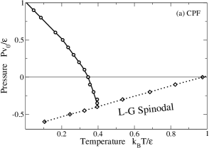
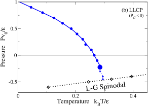
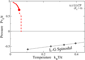
Figure 3: Phase diagrams from MC simulations. We fix the parameters $\tilde{J}=0.5$, $v_{\rm HB}/v_{0}=0.5$ and vary the parameter $\tilde{J}_{\sigma}$. (a) For $\tilde{J}_{\sigma}=0.5$ (i.e. $\tilde{J}_{\sigma}>a+b\tilde{J}$ where $a$ and $b$ are given in the text and both are approximately 1/3), we find a liquid–liquid phase transition (thick line with circles) ending on the superheated liquid-to-gas spinodal (dotted line with diamonds) as in the CPF scenario. (b) For $\tilde{J}_{\sigma}=0.3$ (i.e. $\tilde{J}_{\sigma}>\tilde{J}/2$), the liquid–liquid phase transition ends in a liquid–liquid critical point (LLCP) at negative pressure. (c) For $\tilde{J}_{\sigma}=0.05$ (i.e. $\tilde{J}_{\sigma}<\tilde{J}$), the LLCP ends at positive pressure and the line of specific heat maxima (crosses), emanating from the LLCP, is shown only for positive pressure. Errors are of the order of the symbol sizes. Lines are guides for the eyes. Other model parameters are as for MF calculations (see text).

We simulate this system for $N=10^{4}$ molecules arranged on a square lattice, adopting Wolff’s algorithm to equilibrate at low $T$ mazza , for different values of $\tilde{J_{\sigma}}$, keeping constant $\tilde{J}=0.5$, and $v_{\rm HB}/v_{0}=0.5$ (Fig. 3).

For large values of $\tilde{J_{\sigma}}$ ($\tilde{J_{\sigma}}=0.5>a+b\tilde{J}$), we find a HDL–LDL first–order phase transition that merges with the superheated liquid spinodal as in the CPF scenario (Fig. 3a). At lower $\tilde{J}_{\sigma}$ ($\tilde{J_{\sigma}}=0.3>\tilde{J}/2$), a HDL–LDL critical point appears at $P<0$, from which emanates the locus of $C_{P}$ maxima (used here as an approximation of the liquid–liquid Widom line), which intersects the superheated liquid spinodal (Fig. 3b). By further decreasing $\tilde{J_{\sigma}}$ ($\tilde{J_{\sigma}}=0.05<\tilde{J}/2$), the HDL–LDL critical point occurs at $P>0$, with the line of $C_{P}$ maxima intersecting the $P=0$ axis (Fig. 3c). For $\tilde{J_{\sigma}}=0.02$, approaching zero, we find that the temperature of the HDL–LDL critical point approaches zero and the critical pressure increases toward the value $P=\epsilon/v_{0}$ independent of $\tilde{J}_{\sigma}$. In this case, we can show that Eq. (8) still holds, but with $\tilde{J}^{*}\equiv\tilde{J}$. The line of $C_{P}$ maxima approaches the $T=0$ axis for $\tilde{J}_{\sigma}\rightarrow 0$. These results confirm the qualitative behavior found with the MF calculations.

V Comparison with other thermodynamic models

To show that our analysis offers a general framework within which to analyze the supercooled water phase diagram in terms of the interplay between the strengths of the directional contribution to the H bond interaction and its cooperative part, we compare our results with those from other thermodynamic models that can reproduce more than one scenario by tuning appropriate parameters psgsa ; bds ; tanaka2000 .

One free energy model with cooperative interactions is the one introduced by Tanaka tanaka2000 . He shows that, as in the SF scenario, water’s anomalies are the effect of the excitation of locally favored structures upon cooling, which have lower energy and larger volume than normal-liquid structures. As in our model, in Tanaka’s model increasing the cooperativity among excitations of locally favored structures leads to the LLCP scenario. Moreover, Tanaka’s model LLCP is regulated by relations such as our Eq.(7) and (8). Therefore, by increasing the strength of the cooperative interaction, the LLCP will eventually reach the limit of stability of the liquid, as in the CPF/SL scenario.

We next consider the free energy model introduced by Poole et al. psgsa , in which a van der Waals free energy is augmented to include the effect of H bond formation. The H bond interaction is characterized by two free parameters: the strength of the H bond, and a geometrical constraint on H bond formation. The fraction of molecules that form H bonds with decreased energy and entropy is determined by a distribution over molar volumes, the width of which is $\Delta$. Poole et al. show that, by keeping $\Delta$ fixed, their model displays a SL scenario for weak H bond energy, and a LLCP at positive pressure for strong H bond energy. This corresponds in our model to increase the H bond coupling $\tilde{J}$ from $\tilde{J}<(\tilde{J_{\sigma}}-a)/b$ to $\tilde{J}>2\tilde{J_{\sigma}}$, while keeping $\tilde{J_{\sigma}}>a$ fixed.

Next we study the effect of varying the other H bond parameter in the Poole et al. model, the width $\Delta$. Keeping the H bond energy fixed, we produce the LLCP phase behavior at large $\Delta$ and the SL phase behavior at small $\Delta$. Hence a decrease of $\Delta$ has the same effect on the phase diagram as an increase in the H bond cooperativity in our model.

This result is consistent with that of Borick et al.  bds for their Hamiltonian model that incorporates the cooperativity of H bonds trough the same mechanism used by Poole et al., i.e. by adopting a distribution with width $\Delta$ that makes the H bond strength density dependent. By decreasing $\Delta$, Borick et al. find that the LLCP moves to lower $P$ and higher $T$. This behavior makes sense physically, as a more all-or-nothing distribution of H bonds (small $\Delta$) implies a more cooperative process of bond formation. It also implies that the models of Poole et al. and Borick et al. give rise to the SF scenario only in the limiting case of infinite $\Delta$.

We conclude that all four models give a consistent physical picture. This suggests that our result, expressed in terms of strength of the directional and cooperative components of the H bond, as summarized in Fig. 2, is general.

VI Estimates from experimental data

In the framework of the scheme presented here, in which directionality and cooperativity are the two relvant physical parameters, we propose that the way to understand which scenario best describes water is to probe the energy of the covalent part of the H bond interaction hbond0 and the energy of the cooperative component of the H bond interaction hbond1 ; hbond2 ; hbcoop . Experiments measure H bonds in ice Ih to be approximately 3 kJ/mol stronger than in liquid water newref . Attributing this increase to a cooperative interaction among H bonds energy-coop , we can estimate the value of $J_{\sigma}$ in the cell model to be $\approx$ 1.0 kJ/mol. An estimate of the van der Waals attraction, based on isoelectronic molecules at optimal separation, yields $\epsilon\approx$ 5.5 kJ/mol energy-eps . The optimal H bond energy, $E_{\rm HB}$, has been measured to be $\approx$23.3 kJ/mol suresh . By considering tetrahedral clusters of H bonded molecules, with H bond and van der Waals interactions between n.n. molecules (and appropriately reduced van der Waals interactions between second and third n.n. molecules), we derive the value for the directional component of the H bond, $J\approx$ 12.0 kJ/mol. Other experimental estimates suggest that breaking the directional component of the H bond requires $\approx$ 6.3 kJ/mol newref2 .

Both estimates from experiments fall within the range of $1.1\leq\tilde{J}\leq 2.2$, with $\tilde{J}_{\sigma}\simeq 0.2$, i. e. with $\tilde{J}_{\sigma}<\tilde{J}/2$. Therefore, within our model, these values lead to the LLCP scenario with $P_{C^{\prime}}>0$. In particular, MF calculations with $\tilde{J}_{\sigma}=0.2$, $\tilde{J}=2.2$ and $v_{\rm HB}=2v_{0}$, predict a LLCP at $T_{C^{\prime}}=0.25\epsilon/k_{B}$ and $P_{C^{\prime}}=3.5\epsilon/(v_{0}k_{B})$.

VII Conclusions

We have shown that a microscopic cell model of water, by taking into account the cooperativity among H bonds, is able to produce phase behaviors consistent with any of the proposed scenarios for water’s phase diagram. It is the amount of cooperativity in relation to the strength of the directional component of the H bond that establishes which scenario holds. For no amount of cooperativity, the SF scenario is recovered. By increasing the amount of cooperativity in relation to the H bond directional strength, a liquid–liquid transition grows out from the $T=0$ axis, ending in a LLCP. With sufficiently strong cooperativity, this LLCP lies beyond the region of stable liquid states, leaving only the liquid–liquid transition, consistent with the CPF scenario. In this case the spinodal associated with the transition acts as the line predicted in the SL scenario.

Comparison with previous models gives consistent results. Hence we argue that each of the four scenarios proposed for the phase diagram of liquid water may be viewed as a special case of our general scheme. This scheme is based on the assumption that water-water interaction is characterized by an isotropic component, a directional component and a cooperative component, and that H bond formation leads to an open local structure. Alternative mechanisms, based only on isotropic interactions fmsbs ; jagla ; xu ; f ; deOFNB or only on directional interactions starr have been considered and their relevance for the water case is an open question. Finally, estimates for the three components of the H bond interaction, based on experimental data, lead to the conclusion that the LLCP scenario with a positive critical pressure holds for water.

Figure 1: Phase diagram predicted from MF calculations for the cell model with fixed H bond strength ($\tilde{J}=0.5$), fixed H bond volume increase ($v_{\rm HB}/v_{0}=0.5$), and different values of the H bond cooperativity strength $\tilde{J}_{\sigma}$. (a) Singularity-free scenario ($\tilde{J}_{\sigma}=0$). At high $T$, liquid (L) and gas (G) phases are separated by a first order transition line (thick line) ending at a critical point $C$, from which a L–G Widom line (double–dot–dashed line) emanates. In the liquid phase, maxima of $K_{T}$ and $\alpha_{P}$ converge to a locus (dot–dashed line). At $C^{\prime}$ both $K_{T}$ and $\alpha_{P}$ and have diverging maxima. The locus of the maxima is related to the L-L Widom line for $T_{C^{\prime}}\rightarrow 0$ (see text). (b) Liquid–liquid critical point scenario with positive critical pressure (for $\tilde{J}_{\sigma}=0.05$). At low $T$ and high $P$, a high density liquid (HDL) and a low density liquid (LDL) are separated by a first order transition line (thick line with HDL/LDL labeled) ending in a critical point $C^{\prime}$, from which the L-L Widom line (dot–dashed line) emanates. Other symbols are as in the previous panel. (c) Liquid–liquid critical point scenario with negative critical pressure (for $\tilde{J}_{\sigma}=0.35$). Here the L-L Widom line (dot–dashed line) is shown intersecting the L-G spinodal (dotted line). Other symbols are as in the previous panel. (d) Critical–point free scenario ($\tilde{J}_{\sigma}=0.5$). The HDL–LDL coexistence line extends to the superheated liquid region at $P<0$, reaching with the liquid spinodal (dotted line). The stability limit (SL) of water at ambient conditions (HDL) is delimited by the superheated liquid–to–gas spinodal and the supercooled HDL–to–LDL spinodal (dashed line), giving a re-entrant behavior as hypothesized in the SL scenario. Other symbols are as in the previous panels. In all panels, $k_{B}$ is the Boltzmann constant.

Figure 2: Possible scenarios for water for different values of H bond energies $\tilde{J}$, (directional component) and $\tilde{J}_{\sigma}$ (cooperative component), both in units of the van der Waals energy $\epsilon$, obtained from MF calculations. The ratio $v_{\rm HB}/v_{0}$ is kept constant. (i) If $\tilde{J}_{\sigma}=0$ (red line along x–axis), the singularity free (SF) scenario is realized, independent of $\tilde{J}$. (ii) For large enough $\tilde{J}_{\sigma}$, water would possess a first–order liquid–liquid phase transition line terminating at the liquid–gas spinodal—the critical point free (CPF) scenario; the liquid spinodal would retrace at negative pressure, as in the stability limit (SL) scenario (yellow region in top left). (iii) For other combinations of $\tilde{J}$ and $\tilde{J}_{\sigma}$, water would be described by the liquid–liquid critical point (LLCP) scenario. For larger $\tilde{J}_{\sigma}$, the LLCP is at negative pressure (ochre region between dashed lines). For smaller $\tilde{J}_{\sigma}$, the LLCP is at positive pressure (orange region in bottom right). Dashed lines separating the three different regions correspond to mean field results of the microscopic cell model. Equations for the lines are $\tilde{J}_{\sigma}=\tilde{J}/2$ and $\tilde{J}_{\sigma}=a+b\tilde{J}$, with $a\simeq 0.3$ and $b\simeq 0.36$. The $P-T$ phase diagram evolves continuously as $\tilde{J}$ and $\tilde{J}_{\sigma}$ change.

- (1) Zheligovskaya EA, Malenkov GG (2006) Crystalline water ices. Russian Chem Rev 75:57-76.
- (2) Debenedetti PG (2003) Supercooled and glassy water. J Phys: Condens Matter 15:R1669-R1726.
- (3) Loerting T, Giovambattista N (2006) Amorphous Ice: Experiments and Numerical Simulation. J. Phys: Cond. Mat. 18:R919-R977.
- (4) Kim CU, Barstow B, Tate MW, Gruner SM (2009) Evidence for liquid water during the high-density to low-density amorphous ice transition. Proc Natl Acad Sci USA 106:4597-4600.
- (5) Angell CA (1982) in Water: A Comprehensive Treatise eds Franks F (Plenum, New York), Vol. 7.
- (6) Speedy RJ (1982) Limiting forms of the thermodynamic divergences at the conjectured stability limits in superheated and supercooled water. J Phys Chem 86:3002-3005.
- (7) Poole PH, Sciortino F, Essmann U, Stanley HE (1992) Phase behaviour of metastable water. Nature 360:324-328.
- (8) Starr FW, =Bellisent-Funel MC, Stanley HE (1999) Phys. Rev. E 60:1084.
- (9) Bellissent-Funel MC and L. Bosio (1995) J. Chem. Phys. 102:3727.
- (10) Xu L, Kumar P, Buldyrev SV, Chen S-H, Poole PH, Sciortino F, Stanley HE (2005) Relation between the Widom line and the dynamic crossover in systems with a liquid–liquid phase transition Proc Natl Acad Sci USA 102:16558-16562.
- (11) Poole PH, Sciortino F, Grande T, Stanley HE, Angell CA (1994) Effect of Hydrogen Bonds on the Thermodynamic Behavior of Liquid Water Phys Rev Lett 73:1632-1635.
- (12) Tanaka H (1996) A self-consistent phase diagram for supercooled water Nature 380:328-330.
- (13) Sastry S, Debenedetti PG, Sciortino F, Stanley HE (1996) Singularity-free interpretation of the thermodynamics of supercooled water. Phys Rev E 53:6144-6154.
- (14) Angell CA (2008) Insights into phases of liquid water from study of its unusual glass-forming properties Science 319:582-587.
- (15) Borick SS, Debenedetti PG, Sastry S (1995) A lattice model of network-forming fluids with orientation-dependent bonding - equilibrium, stability, and implications for the phase-behavior of supercooled water. J. Phys. Chem. 11:3781-3792.
- (16) Truskett TM, Debenedetti PG, Sastry S, Torquato S (1999) A single-bond approach to orientation-dependent interactions and its implications for liquid water. J. Chem. Phys. 6:2647-2656.
- (17) Tanaka H, (2000) Thermodynamic anomaly and polyamorphism of water. Europhys. Lett. 50:340-346.
- (18) Franzese G, Stanley HE (2002) Liquid-liquid critical point in a Hamiltonian model for water: analytic solution. J Phys Cond Matter 14:2201-2209.
- (19) Sciortino F, Geiger A, Stanley HE (1991) Effect of Defects on Molecular Mobility in Liquid Water. Nature 354:218-221.
- (20) Sciortino F, Geiger A, Stanley HE (1992) Network Defects and Molecular Mobility in Liquid Water. J. Chem. Phys. 96:3857-3865.
- (21) Pendás AM, Blanco MA, Francisco E (2006) The nature of the hydrogen bond: A synthesis from the interacting quantum atoms picture. J Chem Phys 125:184112.
- (22) Isaacs ED, Shukla A, Platzman PM, Hamann DR, Barbiellini B, Tulk CA (2000) Compton scattering evidence for covalency of the hydrogen bond in ice. J Phys Chem Solids 61:403-406.
- (23) Franzese G, and Stanley HE (2007) The Widom line of Supercooled Water. J Phys: Condens Matter 19:205126.
- (24) Soper AK, Ricci MA (2000) Structures of High-Density and Low-Density Water. Phys. Rev. Lett. 84:2881-2884.
- (25) Ricci MA, Bruni F, Giuliani A (2009) Similarities between confined and supercooled water. Faraday Discuss. 141:347.
- (26) Pedulla JM, Vila F, and Jordan KD (1996) Binding energy of the ring form of (H2O)6: Comparison of the predictions of conventional and localized-orbital MP2 calculations. J Chem Phys 105:11091-11099.
- (27) Kumar R and Skinner JL (2008) Water simulation model with explicit three–molecule interactions. J Phys Chem B 112:8311-8318.
- (28) Ohno K, Okimura M, Akai N, Katsumoto Y (2005) The effect of cooperative hydrogen bonding on the OH stretching-band shift for water clusters studied by matrix-isolation infrared spectroscopy and density functional theory. Phys Chem Chem Phys 7:3005-3014.
- (29) Cruzan JD, Braly LB, Liu K, Brown MG, Loeser JG, Saykally RJ (1996) Quantifying hydrogen bond cooperativity in water: VRT spectroscopy of the water tetramer. Science 271:59-62.
- (30) Schmidt DA, Miki K (2007) Structural correlations in liquid water: A new interpretation of IR spectroscopy. J Phys Chem A 111:10119-10122.
- (31) Sastry S, Sciortino F, Stanley HE (1993) Limits of stability of the liquid-phase in a lattice model with water-like properties. J. Chem. Phys. 12:9863-9872.
- (32) Franzese G, Marqués M, Stanley HE (2003) Intramolecular coupling as a mechanism for a liquid-liquid phase transition. Phys Rev E 67:011103.
- (33) Kumar P, Franzese G, Stanley HE (2008) Predictions of Dynamic Behavior under Pressure for Two Scenarios to Explain Water Anomalies. Phys Rev Lett 100:105701.
- (34) Franzese G, Stanley HE (2002) A theory for discriminating the mechanism responsible for the water density anomaly. Physica A 314:508.
- (35) Kumar P, Franzese G, Stanley HE (2008) Dynamics and thermodynamics of water. J Phys: Condens Matter 20:244114.
- (36) Mazza MG, Stokely K, Strekalova EG, Stanley HE, Franzese G (2009) Cluster Monte Carlo and numerical mean field analysis for the water liquid-liquid phase transition. Comp Phys Comm 180:497-502.
- (37) Rebelo LPN, Debenedetti PG, Sastry S (1998) Singularity-free interpretation of the thermodynamics of supercooled water. II. Thermal and volumetric behavior J. Chem Phys 109 2:626-633.
- (38) Eisenberg D., Kauzmann W. (1969) The Structure and Properties of Water, (Oxford University Press) p. 139.
- (39) Heggie MI, Latham CD, Maynard SCP, and Jones R (1996) Cooperative polarisation in ice Ih and the unusual strength of the hydrogen bond. Chemical Physics Letters 249:485490.
- (40) Henry M (2002) Nonempirical quantification of molecular interactions in supramolecular assemblies ChemPhysChem 3:561-569.
- (41) Suresh SJ, Naik VM (2000) Hydrogen bond thermodynamic properties of water from dielectric constant data J. Chem. Phys. 113:9727-9732.
- (42) Chumaevskii MA, Rodnikova MN (2003) Some peculiarities of liquid water structure, J. Mol. Liq. 106:167-177.
- (43) Franzese G, Malescio G, Skibinsky A, Buldyrev S V, Stanley HE (2001) Generic mechanism for generating a liquid-liquid phase transition. Nature 409:692-695.
- (44) Jagla EA (1999) Core-softened potentials and the anomalous properties of water. J. Chem. Phys. 111:8980.
- (45) Xu L, Kumar P, Buldyrev SV,Chen S-H, Poole PH,Sciortino F, Stanley HE (2005) Relation between the Widom line and the dynamic crossover in systems with a liquid-liquid phase transition. Proc Natl Acad Sci USA 102:16558-16562.
- (46) Franzese G (2007) Differences between discontinuous and continuous soft-core attractive potentials: The appearance of density anomaly. J. Mol. Liq. 136:267.
- (47) de Oliveira AB, Franzese G,Netz PA , Barbosa MC (2008) Waterlike hierarchy of anomalies in a continuous spherical shouldered potential. J. Chem. Phys. 128:064901.
- (48) Hsu CW, Largo J, Sciortino F, Starr FW (2008) Hierarchies of networked phases induced by multiple liquid-liquid critical points. Proc Natl Acad Sci USA 105:13711-13715.