Relative clustering and the joint halo occupation distribution of red-sequence and blue-cloud galaxies in COMBO-17

Abstract

This paper studies the relative spatial distribution of red-sequence and blue-cloud galaxies, and their relation to the dark matter distribution in the COMBO-17 survey as function of scale down to $z\sim 1$. We measure the $2^{\rm nd}$-order auto- and cross-correlation functions of galaxy clustering and express the relative biasing by using aperture statistics. Also estimated is the relation between the galaxies and the dark matter distribution exploiting galaxy-galaxy lensing (GGL). All observables are further interpreted in terms of a halo model. To fully explain the galaxy clustering cross-correlation function with a halo model, we introduce a new parameter, $R$, that describes the statistical correlation between numbers of red and blue galaxies within the same halo.

We find that red and blue galaxies are clearly differently clustered, a significant evolution of the relative clustering with redshift is not found. There is evidence for a scale-dependence of relative biasing: The linear relative bias factor varies slightly between $b\sim 1.7\pm 0.5$ and $b\sim 2.2\pm 0.1$ on spatial scales between roughly $100\,h^{-1}\rm kpc$ and $7\,h^{-1}\rm Mpc$, respectively. The linear correlation coefficient of galaxy number densities drops from a value near unity on large scales to $r\sim 0.6\pm 0.15$. Both biasing trends, the GGL and with some tension the galaxy numbers can be explained consistently within a halo model. Red galaxies typically start to populate haloes with masses starting from $\gtrsim 10^{12.1\pm 0.2}\,h^{-1}{\rm M}_{\odot}$, blue galaxies from $\gtrsim 10^{11.2\pm 0.1}\,h^{-1}{\rm M}_{\odot}$. For the cross-correlation function one requires a HOD variance that becomes Poisson even for relatively small occupancy numbers. This rules out for our samples with high confidence a “Poisson satellite” scenario, as found in semi-analytical models. We compare different model flavours, with and without galaxies at the halo centres, using Bayesian evidence. The result is inconclusive. However, red galaxies have to be concentrated towards the halo centre, either by a red central galaxy or by a concentration parameter above that of dark matter. The value of $R$ depends on the presence or absence of central galaxies: If no central galaxies or only red central galaxies are allowed, $R$ is consistent with zero, whereas a positive correlation $R=+0.5\pm 0.2$ is needed if both blue and red galaxies can have central galaxies.

1 Introduction

Today a confusing wealth of different galaxy populations is known, which yet is thought to have arisen from a fairly simple early Universe. Morphologically, local galaxies fall into two broad classes: early-type galaxies, with almost spheroidal appearance and none or only a very small disk component, and late-type galaxies, with a small central bulge and a dominating stellar disk exhibiting different degrees of spiral structure and star formation. Within the context of the cold dark matter paradigm for cosmological structure formation (Croft et al., 2008; Springel et al., 2005) galaxies merge, grow and interact with the ambient intergalactic medium by participating in a hierarchical merging process (Cole et al., 2000). The ongoing research is trying to test whether the today’s known variety of galaxies can indeed be explained within this paradigm.

To trace the evolution of galaxy populations with time, a morphological identification of a large sample of galaxies down to higher redshifts has proven to be difficult. The most practical solution to this problem is to exploit the bimodal distribution of galaxies in a colour-magnitude diagram (CMD). In such a diagram early- and late-type galaxies can roughly be separated down to redshifts of $z\sim 1$, possibly even beyond that (see e.g. Lin et al., 2008; Faber et al., 2007; Bell et al., 2004, and references therein). The red mode in the CMD is the well-known colour-magnitude relation (CMR), or red-sequence, of early-type galaxies. The blue mode is often referred to as the blue cloud galaxies. To distinguish between a red and a blue galaxy population we proceed according to Bell et al. (2004), using a (rest-frame) $U-V$ vs. $M_{V}$ CMD and cut the galaxy sample along the CMR to obtain a red-sequence and blue-cloud sample. In adopting this division line about $80\%$ of the selected red galaxies have morphologies earlier than or equal Hubble type Sa, while the blue-cloud galaxies are mainly late-type, star forming galaxies. A better morphological separation of galaxies, not pursued for this paper though, may be achieved by applying inclination corrections as discussed in Maller et al. (2008) that have been tested for low-$z$ galaxies from SDSS and 2dF.

The so far strongest observational clues about the emergence of the red-sequence from the blue cloud come from careful number counts in CMDs and estimates of the galaxy luminosity functions for different redshifts. Faber et al. (2007) have found strong evidence that the red-sequence has been built up by a mixture of dry mergers between red-sequence galaxies, wet mergers between blue-cloud galaxies and quenching of star formation with subsequent aging of the stellar populations of blue-cloud galaxies.

Another important source of information hinting to the nature of galaxies is their spatial distribution. For example, early-type galaxies are preferentially found in the cores of rich galaxy clusters where their fraction is about $90$ percent, whereas outside of galaxy clusters about $70$ percent of the field galaxies are late-type galaxies (Dressler, 1980). As another example, it has also been found by modelling stellar populations of local early-types that the star-formation history of early-type galaxies depends on the galaxy density of the environment (Thomas et al., 2005).

One traditional way to study the spatial distribution of galaxies is to look at correlations in the galaxy distribution, in particular the two-point correlation function (Peebles, 1980; Totsuji & Kihara, 1969). Analyses revealed that galaxy clustering depends on the properties of the galaxy population like morphology, colour, luminosity or spectral type (e.g. Coil et al., 2008; Zehavi et al., 2005; Madgwick et al., 2003, and references therein). Therefore, different galaxy populations are differently clustered – biased – with respect to the total matter component and with respect to each other. The detailed dependence of spatial clustering on galaxy characteristics, scale and redshift is a opportunity to learn more about the formation and evolution history of galaxies, see for example White et al. (2007) or Simon (2005a).

Along with this motivation, one aim of this paper is to measure the relative clustering of red (early-type) and blue (late-type) galaxies for different epochs in terms of the linear stochastic biasing parameters. These biasing parameters require $2^{\rm nd}$-order clustering statistics (Dekel & Lahav, 1999). That parametrisation is a completely model-independent, albeit in a statistical sense for non-Gaussian random fields incomplete, measure for comparing two random distributions. It quantifies as function of angular scale the relative clustering strength of two galaxy types and the correlation of their number densities.

The machinery that is applied here to study galaxy biasing is the aperture statistics as formalised in Schneider et al. (1998) and van Waerbeke (1998). It is convenient for analysing weak lensing data and, in particular, to measure the linear stochastic galaxy bias as a function of scale (Simon et al., 2007; Hoekstra et al., 2002). In order to have a compatible statistical measure that quantifies the relative bias between red and blue galaxies the formalism is slightly extended.

Another aim of this paper is to give a physical interpretation of the relative clustering. For that purpose, we use the measurements for setting constraints on parameters of galaxies within the framework of a halo model (van den Bosch et al., 2007; Zheng et al., 2005; Berlind & Weinberg, 2002; Scoccimarro et al., 2001; Seljak, 2000; Peacock & Smith, 2000). In this context, we introduce and discuss a new parameter – the correlation factor of the joint HOD – that regulates the likelihood to find a certain number of red and blue galaxies within the same halo. This allows us to investigate whether two galaxy populations avoid or attract each other inside/inside the same dark matter halo. In Scranton (2003, 2002) a similar modelling is carried out to explain the relative clustering of red and blue galaxy samples, however assuming for simplicity uncorrelated galaxy numbers inside same haloes. In Collister & Lahav (2005) also the clustering of red and blue galaxies was studied by looking at the projected galaxy density profiles of groups.

For the scope of this analysis, the COMBO-17 Survey (Wolf et al., 2004, 2001) offers an unique opportunity. It provides one of the so far largest deep galaxy samples in the redshift regime $0.2\leq z\leq 1.1$ covering an area of $\sim 0.78~{}\rm deg^{2}$, observed in five broad-band and twelve narrow-band filters. Based on the photometry, photometric redshifts of galaxies brighter than $R\leq 24~{}\rm mag$ have been derived within a few percent accuracy as well as absolute rest-frame luminosities and colours. We are analysing the data from three COMBO-17 patches which are known as S11, A901 and CDFS (also known as AXAF).

The survey has also been designed to fit the requirements of gravitational lensing applications (Kleinheinrich et al., 2006; Brown et al., 2003; Gray et al., 2002). The coherent shear distortions of images of background galaxies can therefore be used to infer the relation between galaxy and matter distribution as well (Bartelmann & Schneider, 2001). We use this additional piece of information to further constrain parameters of the halo-model by cross-correlating the COMBO-17 galaxies with the corresponding shear catalogues taken from the Garching-Bonn Deep Survey (GaBoDS) (Hetterscheidt et al., 2007; Erben et al., 2005).

The structure of this paper is as follows. Sect. 2 outlines the quantities that are used to measure the angular galaxy clustering, the aperture ${\cal N}$-statistics. Sect. 3 introduces the COMBO-17-survey and GaBoDS which are the sources of the galaxy samples, red and blue galaxies, and shear catalogues for this study, respectively. Sect. 4 is the place where we describe and present the details of our clustering analysis and compare the results to the literature. The cosmic shear information is harnessed for the GGL, Sect. 5, quantifying the typical matter distribution about the galaxies in our COMBO-17 samples. Sect. 6 outlines the halo model which is then used to interpret the (relative) clustering and the GGL signal of the blue and red galaxy samples. In particular, we introduce and discuss the correlation factor of the joint HOD of two galaxy populations. We finish with a summary in the last section.

Unless stated otherwise we use as fiducial cosmology a $\Lambda$CDM model (adiabatic fluctuations) with $\Omega_{\rm m}=0.24$, $\Omega_{\rm b}=0.0416$, $\Omega_{\Lambda}=1-\Omega_{\rm m}$ and $H_{0}=h\,100\,{\rm km}\,{\rm s}^{-1}\,{\rm Mpc}^{-1}$ with $h=0.732$. The normalisation of the matter fluctuations within a sphere of radius $8\,h^{-1}\rm Mpc$ at redshift zero is assumed to be $\sigma_{8}=0.76$. For the spectral index of the primordial matter power spectrum we use $n_{\rm s}=0.96$. These values are consistent with the third-year WMAP results (Spergel et al., 2007).

2 Clustering quantifiers

2.1 Aperture statistics

The statistics used in this paper to quantify galaxy clustering is the so-called aperture number count statistics. It originally stems from the gravitational lensing literature. As shown in Simon et al. (2007) the aperture number count statistics is useful for studying galaxy clustering even outside the context of gravitational lensing. Its advantage is that no correction for the integral-constraint of the angular correlation function (Peebles, 1980) is needed.

The aperture number count, ${\cal N}({\mn@boldsymbol{\theta}},\theta_{\rm ap})$, measures the fluctuations, excluding shot-noise from discrete galaxies, of the galaxy number density by smoothing the density with a compensated filter $u$, i.e. $\int{\rm d}x\,x\,u(x)=0$:

$${\cal N}({\mn@boldsymbol{\theta}},\theta_{\rm ap})=\frac{1}{\bar{\eta}\theta^{2}_{\rm ap}}\int{\rm d}^{2}{\mn@boldsymbol{\theta}}^{\prime}~{}u\left(\frac{|{\mn@boldsymbol{\theta}}-{\mn@boldsymbol{\theta}}^{\prime}|}{\theta_{\rm ap}}\right)\eta({\mn@boldsymbol{\theta}}^{\prime})\;,$$ (1)

where $\eta({\mn@boldsymbol{\theta}})$ and $\bar{\eta}$ denote the (projected) number density of galaxies in some direction ${\mn@boldsymbol{\theta}}$ and the mean number density of galaxies, respectively. The variable $\theta_{\rm ap}$ defines the smoothing radius of the aperture.

One focus of our analysis is the $2^{\rm nd}$-order statistics of galaxy clustering. All information on the $2^{\rm nd}$-order statistics is comprised by second moments of the aperture number counts as function of $\theta_{\rm ap}$:

$$\big{\langle}{\cal N}_{i}\left(\theta_{\rm ap}\right){\cal N}_{j}\left(\theta_{\rm ap}\right)\big{\rangle}=2\pi\int_{0}^{\infty}{\rm d}\ell\,\ell\,P_{ij}\left(\ell\right)\left[{I}\left(\ell\theta_{\rm ap}\right)\right]^{2},$$ (2)

where $I(x)$ is a filter kernel

$${I}\left(x\right)\equiv\int_{0}^{\infty}{\rm d}s\,s\,u\left(s\right)J_{0}\left(s\,x\right)$$ (3)

to the angular power spectrum $P_{ij}(\ell)$ defined by

$$\frac{\big{\langle}\tilde{\eta}_{i}({\mn@boldsymbol{\ell}}_{1})\tilde{\eta}_{j}({\mn@boldsymbol{\ell}}_{2})\big{\rangle}}{\bar{\eta}_{i}\bar{\eta}_{j}}=(2\pi)^{2}P_{ij}(|{\mn@boldsymbol{\ell}}|)\delta_{\rm D}({\mn@boldsymbol{\ell}}_{1}+{\mn@boldsymbol{\ell}}_{2})\;.$$ (4)

In this equation, $\bar{\eta}_{i}$ is the mean number density of galaxies on the sky, for possibly different galaxy samples. We use $J_{0}(x)$ for the $0^{\rm th}$-order Bessel function of the first kind and $\delta_{\rm D}({\mn@boldsymbol{x}})$ for the Delta-function. The tilde on top of the galaxy number density $\tilde{\eta}$ denotes the angular Fourier transform of $\eta$ assuming a flat sky with Cartesian coordinates which we do throughout this paper:

$$\tilde{\eta}({\mn@boldsymbol{\ell}})=\int{\rm d}^{2}{\mn@boldsymbol{\theta}}\,\eta({\mn@boldsymbol{\theta}})\,{\rm e}^{+{\rm i}{\mn@boldsymbol{\theta}}\cdot{\mn@boldsymbol{\ell}}}~{};~{}\eta({\mn@boldsymbol{\theta}})=\int\frac{{\rm d}^{2}{\mn@boldsymbol{\ell}}}{(2\pi)^{2}}\,\tilde{\eta}({\mn@boldsymbol{\ell}})\,{\rm e}^{-{\rm i}{\mn@boldsymbol{\theta}}\cdot{\mn@boldsymbol{\ell}}}\;.$$ (5)

For $i=j$, $P_{ij}(\ell)$ is an auto-correlation power spectrum, a cross-power spectrum otherwise.

To weigh density fluctuations inside apertures we use a compensated polynomial filter (Schneider, 1998)

$$u\left(x\right)=\frac{9}{\pi}\left(1-x^{2}\right)\left(\frac{1}{3}-x^{2}\right)\,{\rm H}(1-x)\;,$$ (6)

which by definition vanishes for $x\geq 1$; ${\rm H}(x)$ denotes the Heaviside step function. The filter has the effect that only galaxy number density fluctuations from a small range of angular scales contribute to the signal; it acts as a narrow-band filter for the angular modes, $\ell$, with highest sensitivity to $\ell_{\rm c}\approx 1.5\times 10^{4}\,\frac{1^{\prime}}{\theta_{\rm ap}}$. Therefore, the $2^{\rm nd}$-order ${\cal N}$-statistics are essentially a probe for the (band) power spectrum $P_{ij}(\ell_{\rm c})$.

In practice, the ${\cal N}$-statistics are easily derived from the two-point correlation functions, $\omega(\theta)$, of galaxy clustering (e.g. Simon, 2005b) by a weighted integral. As an aside, this is very similar to the approach recently advocated in Padmanabhan et al. (2007) which points out that weighting $\omega(\theta)$ with a compensated filter can also be useful for deprojecting $\omega(\theta)$ to obtain the 3D-correlation function on small cosmological scales.

2.2 Linear stochastic biasing parameters

The linear stochastic biasing parameters (Dekel & Lahav, 1999; Tegmark & Peebles, 1998), expressed here in terms of the ${\cal N}$-statistics, quantify the relative clustering of two random fields, which are in our case the number density of blue and red galaxies:

$$b(\theta_{\rm ap}) = \sqrt{\frac{\big{\langle}{\cal N}^{2}_{\rm red}(\theta_{\rm ap})\big{\rangle}}{\big{\langle}{\cal N}^{2}_{\rm blue}(\theta_{\rm ap})\big{\rangle}}}\;,$$ (7)

$$r(\theta_{\rm ap}) = \frac{\big{\langle}{\cal N}_{\rm red}(\theta_{\rm ap}){\cal N}_{\rm blue}(\theta_{\rm ap})\big{\rangle}}{\sqrt{\big{\langle}{\cal N}^{2}_{\rm red}(\theta_{\rm ap})\big{\rangle}\big{\langle}{\cal N}^{2}_{\rm blue}(\theta_{\rm ap})\big{\rangle}}}\;.$$ (8)

Note that the aperture number count vanishes on average, $\langle{\cal N}\rangle=0$, due to the compensated filter used. Galaxy samples unbiased with respect to each other have $r(\theta_{\rm ap})=b(\theta_{\rm ap})=1$. The parameters are complete for Gaussian random fields, which is only approximately true for large scales but clearly wrong for non-linear scales, effective scale smaller than $\sim 8{\rm Mpc}/h$. Owing to the incomplete picture those biasing parameters convey for the non-Gaussian regime, one is unable to distinguish stochasticity from non-linearity in the relation between the two random fields. Therefore a bias factor $r\neq 1$ can mean a stochastic scatter between galaxy number densities or a non-linear but deterministic mapping (Fry & Gaztanaga, 1993) between number densities – or both. Higher-order statistics or non-Gaussian models for the clustering are required to make this distinction (Wild et al., 2005; Blanton, 2000; Dekel & Lahav, 1999).

Note that the parameter $r(\theta_{\rm ap})$ can be larger than unity because shot-noise contributions to the variances in the aperture galaxy number count are subtracted, or put another way, spatial shot-noise in the fluctuation power of the galaxy number density fields is automatically subtracted as in Guzik & Seljak (2001) or Seljak (2000). The underlying assumption is that galaxies trace a general galaxy number density field by a Poisson sampling process (Poisson shot-noise), which is widely assumed in large-scale structure studies and, in fact, in the definition of the clustering correlation function $\omega(\theta)$.

We employ the linear stochastic biasing parameters here in order to quantify, without too many assumptions, the relative biasing of our blue and red sample as function of scale, $\theta_{\rm ap}$. A more sophisticated and physical, albeit very model-dependent, interpretation of the relative biasing is given within the framework of the halo-model, see Sect. 6.

3 Data set

This study is based on three fields: the S11, A901 and CDFS. The observations of the fields were obtained with the Wide Field Imager (WFI) of the MPG/ESO 2.2m telescope on La Silla, Chile. The camera consists of eight $2\,{\rm k}\times 4\,{\rm k}$ CCDs with a pixel size of $15\,\mu{\rm m}$, corresponding to a pixel scale of $0\hbox{$.\!\!^{\prime\prime}$}238$ in the sky. The field-of-view in the sky is $34^{\prime}\times 33^{\prime}$.

The data from two surveys, carried out with the same instrument, are used. We select blue and red galaxies, possessing photometric redshifts, from the COMBO-17-survey. These data sets are further subdivided into four redshifts bins covering the range between $z=0.2$ and $z=1.0$. Shear catalogues from another survey, GaBoDS, covering the same patches on the sky as COMBO-17, are utilised to quantify the relation between the total (dark) matter density and the galaxy positions by using the gravitational lensing technique. The following sections describe the details of the two surveys and the extracted galaxy and shear catalogues.

3.1 Red and blue galaxy samples: COMBO-17

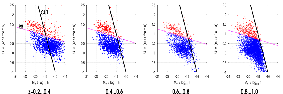
Figure 1: Rest-frame U-V colour vs. absolute magnitude in V-band for the S11 galaxies inside four different redshift ranges (numbers at bottom). Analogous colour-magnitude diagrams for the fields CDFS and A901 look similar. The galaxy sample is split into a red and blue-cloud population by the red-sequence division line “RS”. The steep line “CUT” is an additional cut applied to obtain comparable absolute magnitude-limits in all bins.

The observations and data reduction of the COMBO-17 survey are described in detail in Wolf et al. (2001) and Wolf et al. (2003). Overall the total survey consists of four different, non-contiguous fields observed in 17 optical filters.

The photometric information was used to derive photometric redshifts of galaxies with $m_{R}\lesssim 24~{}\rm mag$, based on a set of galaxy spectrum templates (see references in Wolf et al., 2004). The quality of the estimate depends primarily on the apparent magnitude of the object. As estimator for the redshift uncertainty we use Eq. (5) of Wolf et al. (2004):

$$\sigma_{z}=0.007(1+z)\sqrt{1+10^{0.8(m_{R}-21.6\,{\rm mag})}}\;,$$ (9)

where $\sigma_{z}$ is the 1-$\sigma$ standard deviation of the object redshift. Fig. 2 shows the frequency distribution of the photometric redshifts (solid line) of the full sample.

Based on photometry, rest-frame colours with accuracy $\delta m\sim 0.1~{}\rm mag$ and absolute luminosities with accuracies $\delta m\sim 0.1~{}\rm mag$ ($0.2~{}\rm mag$) for redshifts $z\gtrsim 0.5$ ($\sim 0.3$) were calculated.

Figure 2: Histogram (arbitrary normalisation) of photometric redshifts of galaxies with $m_{\rm R}\leq 24\,\rm mag$ in COMBO-17 (solid line). The mean photometric redshift is $\bar{z}=0.68$. The sample is split into four distinct photo-z bins. The photo-z distribution inside the bins is further convolved with the photo-z error of the individual galaxies to estimate the true redshift distribution inside the photo-z bins (dashed: $\bar{z}=0.3$; dashed-dotted: $\bar{z}=0.5$; dotted: $\bar{z}=0.7$; dashed-dotted-dotted: $\bar{z}=0.9$).

Our object catalogue consists of galaxies with reliable photometric redshifts. Galaxies are only contained in the object catalogue if both spectral classification and estimation of the photometric redshift has been successful. Therefore there is a certain probability with which a galaxy of some absolute magnitude, redshift and template spectrum (SED) cannot be identified. This means that the galaxy sample is incomplete. The completeness of COMBO-17 has been studied using extensive Monte Carlo simulations (Wolf et al., 2003) and has been found to be a complex function of galaxy type and redshift. Roughly, the completeness is about $90\%$ for $m_{R}\lesssim 23~{}\rm mag$ and about $50\%$ near $m_{R}\approx 23.8~{}\rm mag$ (blue, late-type galaxies) or near $m_{R}\approx 23.5~{}\rm mag$ (red, early-type galaxies).

Table 1: Number of galaxies for all redshift bins and survey fields. Only the mean redshifts of the redshift bins $0.2\leq z<0.4$, $0.4\leq z<0.6$, $0.6\leq z<0.8$ and $0.8\leq z<1.0$ are quoted. The quoted fractions are red and blue galaxies (from COMBO-17) relative to the total number of galaxies in the corresponding redshift bin. The comoving number densities derived from the galaxy numbers and the estimated comoving volume of a z-bin and field are corrected for incompleteness. The statistical errors for the individual fields ($2\sigma$) are estimates assuming (uncorrelated) Poisson errors for the absolute galaxy numbers; errors do hence not include cosmic variance for individual fields. The last column contains the number of galaxies (sources) in the shear catalogue (from GaBoDS), with $21.5\leq R<24.5~{}\rm mag$, used for the lensing analysis. The source galaxies have a mean redshift of $\bar{z}=0.78$. The bottom block of the table contains values averaged over all three fields. The errors ($1\sigma$) are now Jackknife-estimates, reflecting cosmic variance derived from the field-to-field variances.

Field	$\bar{z}$	#RED	Fraction	density	#BLUE	Fraction	density	#Sources
				$[10^{-3}h^{3}\rm Mpc^{-3}]$			$[10^{-3}h^{3}\rm Mpc^{-3}]$	(GaBoDS)
A901	$0.31$	$297$	$0.22\pm 0.02$	$10.7\pm 0.6$	$1045$	$0.78\pm 0.02$	$38.3\pm 1.2$	$17084$
	$0.50$	$397$	$0.24\pm 0.02$	$6.2\pm 0.3$	$1264$	$0.76\pm 0.02$	$20.0\pm 0.6$
	$0.71$	$413$	$0.17\pm 0.01$	$3.5\pm 0.2$	$2046$	$0.83\pm 0.01$	$18.2\pm 0.4$
	$0.89$	$376$	$0.13\pm 0.01$	$2.1\pm 0.1$	$2421$	$0.87\pm 0.01$	$12.8\pm 0.3$
CDFS	$0.31$	$118$	$0.16\pm 0.02$	$4.5\pm 0.4$	$621$	$0.84\pm 0.02$	$22.4\pm 0.9$	$20487$
	$0.50$	$338$	$0.18\pm 0.01$	$5.2\pm 0.3$	$1516$	$0.82\pm 0.01$	$23.5\pm 0.6$
	$0.71$	$433$	$0.16\pm 0.01$	$3.8\pm 0.2$	$2323$	$0.84\pm 0.01$	$20.5\pm 0.4$
	$0.89$	$154$	$0.11\pm 0.01$	$0.8\pm 0.1$	$1263$	$0.89\pm 0.01$	$6.8\pm 0.2$
S11	$0.31$	$280$	$0.25\pm 0.02$	$10.4\pm 0.6$	$843$	$0.75\pm 0.02$	$30.3\pm 1.1$	$18996$
	$0.50$	$402$	$0.21\pm 0.01$	$6.4\pm 0.3$	$1518$	$0.79\pm 0.01$	$23.7\pm 0.6$
	$0.71$	$393$	$0.18\pm 0.01$	$3.5\pm 0.2$	$1832$	$0.82\pm 0.01$	$16.3\pm 0.4$
	$0.89$	$367$	$0.14\pm 0.01$	$2.0\pm 0.1$	$2334$	$0.86\pm 0.01$	$12.4\pm 0.3$
COMBINED	$0.31$	.	$0.21\pm 0.08$	$8.5\pm 3.0$	.	$0.79\pm 0.08$	$30.3\pm 6.9$
	$0.50$	.	$0.21\pm 0.05$	$5.9\pm 0.6$	.	$0.79\pm 0.05$	$22.4\pm 1.8$
	$0.70$	.	$0.17\pm 0.02$	$3.6\pm 0.2$	.	$0.83\pm 0.02$	$18.3\pm 2.8$
	$0.89$	.	$0.13\pm 0.03$	$1.6\pm 0.6$	.	$0.87\pm 0.03$	$10.7\pm 2.9$

We split the total object catalogue into four distinct photo-z bins, namely a) $0.2\leq z<0.4$, b) $0.4\leq z<0.6$, c) $0.6\leq z<0.8$ and d) $0.8\leq z<1.0$. The mean redshifts of galaxies belonging to a)-d) are $\bar{z}=0.3,0.5,0.7,0.9$, respectively. The sizes of the samples are listed in Table 1.

In order to have a better estimate for the true redshift distribution, the photo-z distribution of every bin is convolved with the photo-z error (Gaussian errors) of the individual galaxies, Eq. (9). The average redshift uncertainties are $\sigma_{z}=0.02,0.04,0.06,0.08$ for the samples a)-d), respectively. See Fig. 2 for the resulting distributions. Obviously, the true redshift distribution is wider than the photo-z distribution. Ignoring this effect would lead to a systematic under-estimation of the galaxy clustering amplitude by $\sim 20\%$ (Brown et al., 2008).

The galaxy samples are further subdivided by applying a cut in the rest-frame $U-V$ vs. $M_{V}-5\,\log_{10}h$ CMD (Johnson filter) along the line

$$(U-V)(M_{V},z)=$$ (10)

$$1.15-0.31\,z-0.08(M_{V}-5\log_{10}h+20)\;.$$

This model-independent, empirical cut has been chosen by Bell et al. (2004) to study red galaxies near the galaxy red-sequence. It slices the bimodal distribution of galaxies in the CMD between the two modes. Galaxies redder than $(U-V)(M_{V},z)$ are dubbed “red galaxies”, “blue galaxies” otherwise. For the redshifts considered here, most of the red galaxies selected this way are morphologically early-type with dominant old stellar populations, while blue galaxies are mainly late-type, star-forming galaxies.

The redshift dependence of the CMR zero-point, in Eq. (10), was fitted to match the colour evolution of COMBO-17 early-type galaxies and to be consistent with the SDSS CMR zero-point at low redshift. From the viewpoint of the COMBO-17 early-types the zero-point for redshifts $z\lesssim 0.2$ is slightly too low, giving a small contamination of the red sample with blue cloud galaxies. Since we consider only galaxies starting from $z\geq 0.2$, this contamination is negligible for this study, though.

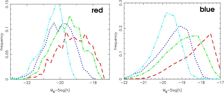
Figure 3: Frequency distribution of (rest-frame) B-band magnitudes, separated for red (left) and blue (right) galaxies, for the four different photo-z bins (dashed lines: $\bar{z}=0.3$; dashed-dotted: $\bar{z}=0.5$; dotted: $\bar{z}=0.7$; dashed-dotted-dotted: $\bar{z}=0.9$). The corresponding mean magnitudes and standard deviations in order of increasing mean redshifts are ($h=1$): $\langle M_{\rm B}\rangle=-19.20\pm 0.94\,{\rm mag},-19.56\pm 0.91\,{\rm mag},-20.06\pm 0.84\,{\rm mag},-20.49\pm 0.68\,{\rm mag}$ (red) and $\langle M_{\rm B}\rangle=-18.34\pm 0.88\,{\rm mag},-18.96\pm 0.94\,{\rm mag},-19.46\pm 0.83\,{\rm mag},-19.83\pm 0.69\,{\rm mag}$ (blue).

As we took only galaxies with reliable photometric redshifts, we have as further selection rule $m_{\rm R}\leq 24\,\rm mag$. The distribution of our samples in a rest-frame CMD is plotted in Fig. 1. Obviously, in the lowest redshift bin CMD galaxies populate faint regions in the diagram that are excluded in the other redshift bins due to the survey flux-limit. We estimate that in the three deeper redshift bins galaxies have roughly to be brighter than (rest-frame)

$$M_{\rm V}-5\log_{10}h\approx-17\,\rm mag-(U-V)$$ (11)

in order to be included (see steep black lines in Fig. 1). To acquire comparable galaxy samples at all redshifts we artificially apply this limit as cut to all redshift bins. After applying this cut, the galaxy samples of all redshift bins have comparable absolute rest-frame $M_{V}$ luminosities. The red sample has an average of $\langle M_{V}\rangle=-20.0\pm 0.1\,\rm mag$, the blue sample $\langle M_{V}\rangle=-18.8\pm 0.3\,\rm mag$ (for $h=1$).

In contrast to the red-sequence cut, this luminosity cut does not take into account the colour/luminosity evolution of the samples but is placed at the same position of the rest-frame CMD-diagram at all redshifts. We therefore expect the selected galaxy populations of all redshifts not to be totally equivalent at the faint end. For an easier comparison with the literature, e.g. Brown et al. (2008), Fig. 3 shows also the distribution of rest-frame $M_{\rm B}$-magnitudes of the various samples. The samples become bluer with increasing redshift which is, at least partially, explained by the passive evolution of the stellar populations.

We determine the absolute number density, $\phi_{\rm type}$, of our galaxy samples by using the $\rm V_{max}$-estimator (e.g. Fried et al., 2001). This estimator needs to be slightly modified since we are not selecting the galaxies from a top-hat redshift range. Instead we are selecting, for every photo-z bin, galaxies in redshift with a probability proportional to $p(z)$, which is the aforementioned photo-z distribution convolved with the photo-z error; $p(z)$ resembles only for the lowest z-bin roughly a top-hat selection window, see Fig. 2. Due to the uncertainty in redshift we also select galaxies from a redshift range (volume) larger than the photo-z window would imply. Not taking this effect into account would mean to over-estimate the galaxy number density. Assuming that we are selecting, apart from the incompleteness expressed by the incompleteness function $C(z,{\rm SED},U-V,R)$ (Wolf et al., 2003), all galaxies at the redshift of maximum $p(z)$, $p_{\rm max}$ say, the $V_{\rm max}$-estimator is:

$$\!\!\!\phi_{\rm type}=\sum_{i=1}^{N_{\rm gal}}\frac{1}{V_{i}}~{};~{}\sigma^{2}(\phi_{\rm type})=\sum_{i=1}^{N_{\rm gal}}\frac{1}{V^{2}_{i}}\;,$$ (12)

$$\!\!\!V_{i}\equiv$$ (13)

$$\frac{\Omega}{p_{\rm max}}\int_{0}^{\infty}{\rm d}z\,p(z)\,\frac{dV}{d\Omega{\rm d}z}\,C(z,{\rm type},U_{i}-V_{i},R_{i})\;.$$ (14)

Therefore, $p(z)$ is used here to correct the incompleteness function $C$ for our additional galaxy redshift selection criterion. By $\Omega$ we denote the survey area of a COMBO-17-patch which is $\Omega=f\times(39.7\,\rm arcmin)^{2}$ with a filling factor $f$, estimated from the patch masks, of $f=0.56,0.54,0.55$ for A901, CDFS and S11, respectively. The estimator $\sigma^{2}(\phi_{\rm type})$ is used for the Poisson shot-noise error of $\phi_{\rm type}$. For a top-hat selection function $p(z)$, one obtains the estimator mentioned in Fried et al.

3.2 Cosmic shear data: GaBoDS

The data reduction of GaBoDS was performed with a nearly fully automatic, stand-alone pipeline which we had developed to reduce optical and near infrared images, especially those taken with multi-chip cameras. Since weak gravitational lensing was our main science driver, the pipeline algorithms were optimised to produce deep co-added mosaics from individual exposures obtained from empty field observations. Special care was taken to achieve an accurate astrometry to reduce possible artificial PSF patterns in the final co-added images. For the co-addition we used the programme EISdrizzle. A detailed description of the pipeline can be found in Erben et al. (2005).

The shape of galaxies is influenced by the anisotropic PSF. In order to obtain unbiased shear estimates from observed source galaxy ellipticities we use the so-called KSB algorithm (Kaiser et al., 1995). For a detailed description of our implementation of the KSB-algorithm and catalogue creation we refer the reader to Hetterscheidt et al. (2007). Our KSB-algorithm pipeline was blind-tested with simulated data within the STEP project (Massey et al., 2007; Heymans et al., 2006).

For the PSF-anisotropy correction we utilise stars which are point-like and unaffected by lensing. By using a sample of bright, unsaturated stars, we measure the anisotropic PSF with a Gaussian filter scale matched to the size of the galaxy image to be corrected (Hoekstra et al., 1998). In the case of the WFI@2.2m instrument the PSF of the co-added images varies smoothly over the total field-of-view. Therefore we perform a third-order two-dimensional polynomial fit to the PSF anisotropy with $3.5\,\sigma$-clipping as a function of position over the entire field-of-view. With this fit it is possible to estimate the PSF anisotropy at the position of the galaxies.

All objects for which problems concerning the determination of shape or centroid position occur are rejected (e.g. objects near the border, with negative total flux, with negative semi major and/or semi major axis). In addition, we only use those objects with a half-light radius which is larger than that measured for stars and an ellipticity (after PSF correction) of less than $1.0$. Additionally, we only use those galaxies with a signal-to-noise ratio larger than five, since a comparison of ground- and space-based data showed that galaxies with a lower S/N do not contain any shear information (Hetterscheidt et al., in prep.). We adopt the scheme in Erben et al. (2001) and Hetterscheidt et al. (2005) to estimate uncertainties for each galaxy ellipticities. In the following lensing analysis galaxies are weighted with the inverse of the square of the estimates variances.

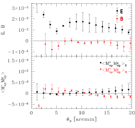
Figure 4: Various measurements of the aperture mass statistics of the three COMBO-17-fields in $R$-band ($\approx 0.75\,{\rm deg}^{2}$). All galaxies in the magnitude range $R\in[21.5,24.5]$ are used for the cosmic shear analysis. The effective number density of galaxies is $16\,{\rm arcmin}^{-2}$. The error-bars denote the field-to-field variance between the three fields. Upper panel: E- and B-mode decomposition of the $M_{\rm ap}$-signal. Lower panel: Cross-correlation between uncorrected stars- and corrected galaxies for E- and B-modes.

A powerful way to reveal possible systematic errors in the PSF-correction is the application of the aperture mass statistics as it provides an unambiguous splitting of E- and B-modes:

$$\big{\langle}M_{\rm ap,\perp}^{2}(\theta_{\rm ap})\big{\rangle}=$$ (15)

$$\frac{1}{2}\int_{0}^{2\theta_{\rm ap}}\frac{{\rm d}\theta\,\theta}{\theta_{\rm ap}^{2}}\left[\xi_{+}(\theta)\,T_{+}\left(\frac{\theta}{\theta_{\rm ap}}\right)\pm\xi_{-}(\theta)\,T_{-}\left(\frac{\theta}{\theta_{\rm ap}}\right)\right]\;.$$

The $M_{\rm ap}$-statistics quantify the fluctuations of the shear signal (E-mode: plus sign on r.h.s, B-mode: minus sign) within an aperture of radius $\theta_{\rm ap}$. They can be obtained by transforming the shear-shear correlation functions $\xi_{\pm}$ (e.g. Hetterscheidt et al., 2007). We use $T_{\pm}$ as derived in Schneider et al. (2002). The presence of non-vanishing B-modes is a good indicator for systematics arising, for instance, from an imperfect anisotropy correction.

However, there are several possible astronomical sources of B-modes, like the intrinsic alignment of galaxies (e.g. Heavens et al., 2000; Heymans & Heavens, 2003), the intrinsic shape-shear correlation (e.g. Hirata & Seljak, 2004; Heymans et al., 2006) and the redshift clustering of source galaxies (Schneider et al., 2002). Furthermore, Kilbinger et al. (2006) found in their work a mixing of E- and B-modes due to a cut off in $\xi_{\pm}$ on small angular scales. However, all those B-mode sources are expected to be much smaller than the statistical errors of the three fields and are therefore irrelevant in the following analyses.

A further method to check for systematics is the cross-correlation between PSF-uncorrected stars and anisotropy corrected galaxies (e.g. Bacon et al., 2003). For that purpose, shear-shear cross-correlations, $\xi_{\pm}$, between star-ellipticities and galaxy-ellipticities are computed and transformed according to Eq. (15). We denote the thereby obtained $M_{\rm ap}$-variances as $M_{\rm cross;E}$ and $M_{\rm cross;B}$ for the E- and B-modes, respectively.

In Fig. 4 the average E- and B-mode signal and the average signal of the cross-correlation between anisotropy-corrected stars and uncorrected galaxies, $M_{\rm cross;E}$ and $M_{\rm cross;B}$, are displayed (further details on $M_{\rm cross;E}$ and $M_{\rm cross;B}$ are given in Hetterscheidt et al., 2007). The measured B-mode signal is consistent with zero within the $1\,\sigma$-range for $\theta_{0}>2^{\prime}$, and the cross-correlation between uncorrected stars and corrected galaxies, $M_{\rm cross;B}$, is consistent with, or close to zero. Hence the B-mode signal does not indicate an imperfect anisotropy correction. Additionally, the cross-correlation signal, $M_{\rm cross;E}$ is consistent with zero.

Taking the B-modes and the cross-correlation signals $M_{\rm cross;E}$ and $M_{\rm cross;B}$ into account we conclude that the influence of systematics on the calculated E-mode signal is negligible compared to statistical errors.

4 Relative biasing of red and blue galaxies

4.1 Combining measurements

We outline here how measurements of the same quantity in the $N_{\rm p}=3$ different fields were combined, and how the covariance of the combined value was estimated.

The quantities estimated from the data, as function of galaxy-galaxy separation on the sky, are the angular clustering of the galaxy samples, in terms of the aperture statistics (auto- and cross-correlations), and later on the mean tangential shear around the galaxies. The measurements are binned into five logarithmic angular bins and compiled as a data vector ${\mn@boldsymbol{d}}_{i}$, where $i=1\ldots 3$ is an index for the survey field (either A901, S11 or CDFS).

A commonly applied technique for combining all measurements and estimating the covariance of the combination is by looking at the field-to-field variance of ${\mn@boldsymbol{d}}_{i}$ (e.g. Hetterscheidt et al., 2007). Applying this technique to mere three fields, however, poses problems that are unsolved so far (Hartlap et al., 2007) and would bias the final results. We therefore use a different approach here.

For each field $i$ individually, the measurement is repeated $N_{\rm b}=100$ times on bootstrapped data, which is acquired by randomly drawing galaxies (with replacement) from the original samples. The size of the bootstrap samples equals the the size of the original sample. For a recent paper on this and related statistical tools for error estimation see Norberg et al. (2008), which points bootstrapping out as appropriate, albeit conservative (errors are overestimated by $\sim 40\%$), method for uncertainties in two-point correlation functions.. The data vector of the $j$-th bootstrapped sample of the $i$-th field is denoted by ${\mn@boldsymbol{d}}_{ij}$. The variance of ${\mn@boldsymbol{d}}_{i}$ among the bootstrap samples yields an estimate for the covariance of the statistical errors in ${\mn@boldsymbol{d}}_{i}$ due to galaxy shot noise:

$$\textbf{{C}}_{i}=\frac{1}{N_{\rm b}-1}\sum_{j=1}^{N_{\rm b}}\left({\mn@boldsymbol{d}}_{ij}-{\mn@boldsymbol{d}}_{i}\right)\left({\mn@boldsymbol{d}}_{ij}-{\mn@boldsymbol{d}}_{i}\right)^{\rm t}\;.$$ (16)

The most likely value of a combined ${\mn@boldsymbol{d}}$ of all fields, constrained by all individual ${\mn@boldsymbol{d}}_{i}$ and their covariances $\textbf{{C}}_{i}$, is

$${\mn@boldsymbol{d}}=\textbf{{C}}\sum_{i=1}^{N_{\rm p}}\left[\textbf{{C}}_{i}\right]^{-1}{\mn@boldsymbol{d}}_{i}~{};~{}\textbf{{C}}\equiv\left[\sum_{i=1}^{N_{\rm p}}\left(\textbf{{C}}_{i}\right)^{-1}\right]^{-1}\;,$$ (17)

obtained by finding the minimum of ${\mn@boldsymbol{d}}$ in the negative log-likelihood (assuming Gaussian errors):

$$\frac{\partial\chi^{2}({\mn@boldsymbol{d}})}{\partial{\mn@boldsymbol{d}}}=0~{};~{}\chi^{2}({\mn@boldsymbol{d}})\equiv\sum_{i=1}^{N_{\rm p}}\left({\mn@boldsymbol{d}}_{i}-{\mn@boldsymbol{d}}\right)^{\rm t}\left[\textbf{{C}}_{i}\right]^{-1}\left({\mn@boldsymbol{d}}_{i}-{\mn@boldsymbol{d}}\right)\;.$$ (18)

This is the generalisation of the well-known rule to combine measurements by inversely weighting with their statistical error. We consider the assumption of Gaussian statistics for the likelihood function as valid approximation for the following reasons:

• The statistical errors of the angular clustering estimator, outlined below, are known to be Poisson, hence closely Gaussian for a not too small number of galaxy pairs inside a bin (Landy & Szalay, 1993). Since we linearly combine different, little correlated, angular bins of the clustering estimator to obtain the $\cal N$-statistics, the $\cal N$-estimates are even more Gaussianly distributed according to the central limit theorem of statistics.

• As for GGL, the complex ellipticities of the lensed sources obey roughly a bivariate Gaussian distribution which makes the estimate for GGL inside an angular bin also approximately Gaussianly distributed.

Even if the noise in the data does not obey Gaussian statistics, the l.h.s. estimator Eq. (17) yields an unbiased however not optimal (maximum likelihood) estimate of ${\mn@boldsymbol{d}}$, with C as covariance, as any weighted average of unbiased estimates ${\mn@boldsymbol{d}}_{i}$ is itself an unbiased estimator.

As pointed out by Hartlap et al. (2007) taking the inverse of the (bootstrapped) $\textbf{{C}}_{i}$ gives a biased estimate of the inverse. To obtain an unbiased estimator of the inverse we multiply $\textbf{{C}}_{i}$ in Eq. (16) by the factor:

$$\frac{N_{\rm b}}{N_{\rm b}-p-1}\;,$$ (19)

where $p$ is the size of the vector ${\mn@boldsymbol{d}}$ (here: $p=15$, five angular bins for $\langle{\cal N}_{\rm red}^{2}\rangle$, $\langle{\cal N}_{\rm blue}^{2}\rangle$, $\langle{\cal N}_{\rm red}{\cal N}_{\rm blue}\rangle$, respectively; for the halo-model fit later on we will extend ${\mn@boldsymbol{d}}_{i}$ by ten more components comprising the GGL signal of the samples).

The covariance of the combined mean ${\mn@boldsymbol{d}}$ is simply

$$\langle{\mn@boldsymbol{d}}{\mn@boldsymbol{d}}^{\rm t}\rangle-\langle{\mn@boldsymbol{d}}\rangle\langle{\mn@boldsymbol{d}}\rangle^{\rm t}=\textbf{{C}}\;.$$ (20)

This covariance does not contain an estimate of the cosmic variance, though, because it is solely based on bootstrapping using individual fields (galaxy shot-noise) and does not include a field-to-field variance between the fields.

This can be seen by considering a toy example which has just one bin, $d_{i}$, for the field data vectors and equal (co)variance for all fields, $C_{i}=\sigma^{2}$ say. The above equations tell us for that case that $d$ is the arithmetic mean of all $d_{i}$, and the combined variance is $C=\sigma^{2}N_{\rm p}^{-1}$. Based on this, if we had an infinite number of galaxies within each field, i.e. bootstrapped $\sigma\rightarrow 0$, we would expect a “perfect” measurement with $C=0$. Hence, $C$ completely ignores the possibility that $d_{i}\neq d_{j}$ for $i\neq j$ even with a hypothetically infinite number of galaxies inside each patch (cosmic variance).

We expect the actual uncertainty therefore to be somewhat higher than expressed by C, especially for the larger separation bins (larger aperture radii) where cosmic variance errors are becoming larger with respect to shot-noise errors. The fact that the bootstrap variances overestimate the covariance presumably compensates this deficit to some extend.

4.2 Clustering of red and blue galaxies

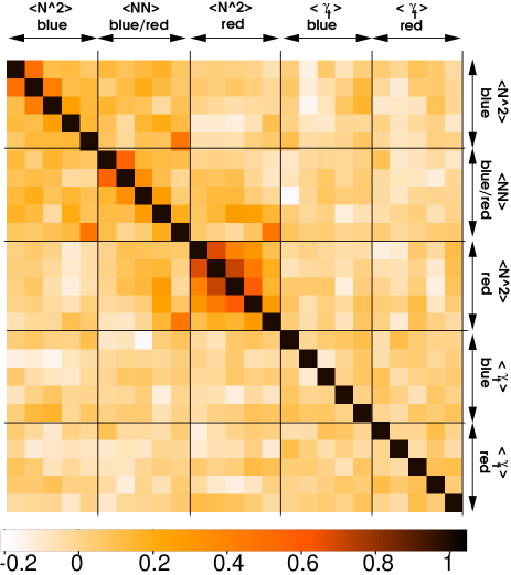
Figure 5: Correlation of statistical errors of the aperture number count statistics – $\langle{\cal N}^{2}_{\rm blue}\rangle$, $\langle{\cal N}_{\rm blue}{\cal N}_{\rm red}\rangle$ and $\langle{\cal N}^{2}_{\rm red}\rangle$ for five aperture radii each – and the GGL signal – $\langle\gamma_{\rm t}\rangle$ for the blue and red sample – for a mean redshift of $z=0.7$ as obtained from bootstrapping the data. The correlation matrix for the other redshift bins look similar.

4.2.1 Method

The ${\cal N}$-statistics is derived from the angular clustering of the galaxy samples, $\omega(\theta)$ (Peebles, 1980), by a linear transformation (Simon et al., 2007)

$$\langle{\cal N}_{i}(\theta_{\rm ap}){\cal N}_{j}(\theta_{\rm ap})\rangle=\int_{0}^{2}{\rm d}x\,x\,\omega_{ij}(\theta_{\rm ap}\,x)\,T_{+}(x)\;,$$ (21)

where

$$T_{+}\left(x\right)\equiv\left(2\pi\right)^{2}\int_{0}^{\infty}{\rm d}s~{}s~{}\left[\rm I\left(s\right)\right]^{2}J_{0}\left(sx\right)\;.$$ (22)

The indices $i$ and $j$ are used to denote the different galaxy samples. For estimating the angular clustering of a single sample, $i=j$, we use the standard method of counting the number of galaxy pair within a certain separation, namely pairs of galaxies from the same sample, $\langle DD\rangle$, pairs of galaxies from a random mock sample and the COMBO-sample, $\langle DR\rangle$, and pairs between galaxies from the same mock sample, $\langle RR\rangle$ (Landy & Szalay, 1993). The number of pairs involving random mock samples is averaged over $50$ mock realisations for each correlation function.

For the random catalogue, we assume that the completeness of the galaxies inside a redshift is homogeneous, so that the only relevant parameters for the random mocks is the number of galaxies and the masking, which is applied for all galaxies equally.

The cross-correlation function, $i\neq j$, is computed implementing the estimator (Szapudi & Szalay, 1997):

$$\omega_{ij}(\theta)=\frac{\langle D_{i}D_{j}\rangle}{\langle R_{i}R_{j}\rangle}-\frac{\langle D_{i}R_{j}\rangle+\langle D_{j}R_{i}\rangle}{\langle R_{i}R_{j}\rangle}+1\;,$$ (23)

for which counting the number of pairs between different galaxy samples, $D_{i/j}$, and different mock samples, $R_{i/j}$, is required. For example, $\langle R_{i}D_{j}\rangle$ denotes the number of pairs between galaxies from a $i$-mock catalogue and galaxies $j$ within a certain $\theta$ separation interval. Note that the size of the mock sample $R_{k}$ is the same as the size of the galaxy sample $D_{k}$.

Traditionally, galaxy clustering is studied using the angular correlation function $\omega(\theta)$. For a comparison of our results for the two-point statistics of galaxy clustering in COMBO-17 with the literature, we infer the angular correlation function from the ${\cal N}$-statistics by applying the method outlined in Simon et al. (2007). This method allows us to be ignorant about the integral constraint which offsets the estimates of $\omega(\theta)$ obtained from the aforementioned estimators. We parameterise $\omega(\theta)$ as a simple power-law

$$\omega(\theta)=A_{\omega}\,\left(\frac{\theta}{1^{\prime}}\right)^{-\delta}\;;$$ (24)

$A_{\omega}$ and $\delta$ are constants. Moreover, we deproject $\omega(\theta)$ in order to obtain an average 3D-correlation function for the clustering of the samples,

$$\xi(r)=\left(\frac{r}{r_{0}}\right)^{-\delta-1}\;,$$ (25)

after having made sure that the Limber approximation (Peebles, 1980; Limber, 1953) was valid here (Simon, 2007); the constant $r_{0}$ is the correlation length.

As the 2D-correlation functions are not exactly power-laws (Zehavi et al., 2004), the foregoing procedure will yield parameters for the 3D-clustering which are biased to some extent. We do not discuss this effect further but point out here that this bias could, in principle, be estimated from the halo-model fit, which also predicts the 3D-correlation function.

Figure 6: Variance of the aperture number count, $\langle{\cal N}_{\rm red}^{2}\rangle$ and $\langle{\cal N}_{\rm blue}^{2}\rangle$, for red (filled circles) and blue (filled stars) galaxies. The straight lines are the best-fitting power laws to the measurements. The thick solid line denotes the theoretical variance for galaxies unbiased to the dark matter (as in Smith et al., 2003). Also plotted is the aperture number count cross-correlation, $\langle{\cal N}_{\rm red}{\cal N}_{\rm blue}\rangle$, between blue and red galaxies (open stars). The data points are slightly shifted along the abscissa to increase the visibility.

Table 2: The results are for $\Omega_{\rm m}=0.3$, $\Omega_{\Lambda}=0.7$. Upper half of table: summary of results (median and $68\%$ confidence levels) obtained considering values for $\langle{\cal N}^{2}\rangle$ out of $\theta\in[0.1^{\prime},23^{\prime}]$ for red and blue galaxies for different mean redshifts, $\bar{z}$. Note that the statistical errors of $\delta$ and $A_{\omega}$ are strongly anti-correlated with a correlation coefficient of about $-0.6$. Lower half of table: the fit for $\omega(\theta)$ has been transformed into the 3D-galaxy clustering function $\xi(r)=(r/r_{0})^{-\gamma}$ using Limber’s equation. The clustering length $r_{0}$ is in units of $h^{-1}\rm Mpc$; $\xi_{1\rm Mpc}$ denotes $\xi(r)$ at a comoving length of $r=1\,h^{-1}\rm Mpc$. Parameters with a “$|\delta$”-suffix are fits for a fixed slope: $\delta=0.85,0.65$ for red and blue, respectively.

	RED SAMPLE					BLUE SAMPLE
$\bar{z}$	$[A_{\omega}$	$\delta$	$\chi^{2}/n$	$A_{\omega}|\delta$	$\chi^{2}/n$]	$[A_{\omega}$	$\delta$	$\chi^{2}/n$	$A_{\omega}|\delta$	$\chi^{2}/n]$
0.31	$0.46_{-0.14}^{+0.15}$	$0.81_{-0.27}^{+0.19}$	$0.3$	$0.47^{+0.12}_{-0.12}$	$0.2$	$0.11_{-0.04}^{+0.20}$	$0.49_{-0.39}^{+0.35}$	$1.2$	$0.09^{+0.02}_{-0.02}$	$0.8$
0.50	$0.27_{-0.07}^{+0.07}$	$0.97_{-0.16}^{+0.13}$	$2.4$	$0.29^{+0.06}_{-0.06}$	$3.0$	$0.08_{-0.02}^{+0.02}$	$0.76_{-0.13}^{+0.12}$	$3.8$	$0.09^{+0.02}_{-0.02}$	$4.5$
0.70	$0.44_{-0.09}^{+0.09}$	$0.85_{-0.17}^{+0.14}$	$0.6$	$0.45^{+0.07}_{-0.07}$	$0.6$	$0.08_{-0.02}^{+0.02}$	$0.67_{-0.14}^{+0.12}$	$2.3$	$0.08^{+0.01}_{-0.01}$	$2.3$
0.90	$0.31_{-0.11}^{+0.16}$	$0.69_{-0.44}^{+0.31}$	$0.7$	$0.28^{+0.08}_{-0.08}$	$0.4$	$0.08_{-0.03}^{+0.27}$	$0.33_{-0.27}^{+0.30}$	$1.3$	$0.05^{+0.01}_{-0.01}$	$0.8$
$\bar{z}$	[$r_{0}$	$\gamma$	$\xi_{1\rm Mpc}$	$r_{0}|\delta$	$\xi_{1\rm Mpc}|\delta$]	[$r_{0}$	$\gamma$	$\xi_{1\rm Mpc}$	$r_{0}|\delta$	$\xi_{1\rm Mpc}|\delta$]
0.31	$5.37_{-1.54}^{+2.72}$	$1.81_{-0.27}^{+0.19}$	$20.6_{-6.9}^{+7.4}$	$5.19^{+0.67}_{-0.74}$	$21.0^{+5.3}_{-5.2}$	$2.98_{-1.12}^{+2.74}$	$1.49_{-0.39}^{+0.35}$	$5.0_{-2.0}^{+2.5}$	$2.50^{+0.38}_{-0.42}$	$4.6^{+1.2}_{-1.2}$
0.50	$4.37_{-0.86}^{+1.06}$	$1.97_{-0.16}^{+0.13}$	$17.8_{-4.7}^{+4.9}$	$5.04^{+0.56}_{-0.62}$	$19.9^{+4.3}_{-4.3}$	$2.66_{-0.51}^{+0.57}$	$1.76_{-0.13}^{+0.12}$	$5.6_{-1.4}^{+1.5}$	$3.08^{+0.35}_{-0.38}$	$6.4^{+1.2}_{-1.2}$
0.70	$7.43_{-1.42}^{+2.00}$	$1.85_{-0.17}^{+0.14}$	$40.3_{-7.7}^{+7.9}$	$7.51^{+0.66}_{-0.71}$	$41.7^{+7.0}_{-7.0}$	$3.20_{-0.51}^{+0.59}$	$1.67_{-0.14}^{+0.12}$	$6.9_{-0.6}^{+1.3}$	$3.30^{+0.29}_{-0.31}$	$7.2^{+1.1}_{-1.1}$
0.90	$7.60_{-2.41}^{+5.20}$	$1.69_{-0.44}^{+0.31}$	$28.7_{-9.25}^{+10.3}$	$6.58^{+0.94}_{-1.07}$	$32.7^{+9.19}_{-9.17}$	$3.52_{-0.97}^{+1.82}$	$1.33_{-0.27}^{+0.30}$	$5.5_{-1.4}^{+1.4}$	$2.70^{+0.33}_{-0.36}$	$5.1^{+1.1}_{-1.1}$

4.2.2 Results

The combined measurements of the $2^{\rm nd}$-order ${\cal N}$-statistics for blue and red galaxies can be found in Fig. 6. The ${\cal N}$-statistics is binned between $0^{\prime}.1\leq\theta_{\rm ap}<23^{\prime}$ using five logarithmic bins. The statistical errors are somewhat correlated which can be seen in Fig.5. The best fits of the angular clustering and 3D-clustering parameters are listed in Table 2. Averaging over all redshift bins, we find for the red sample $A_{\omega}=0.35\pm 0.06$, $\delta=0.85\pm 0.10$ and $r_{0}=5.5\pm 0.9\,h^{-1}\rm Mpc$. The corresponding values of the blue sample are $A_{\omega}=0.08\pm 0.02$, $\delta=0.65\pm 0.08$ and $r_{0}=3.0\pm 0.4\,h^{-1}\rm Mpc$. If we combine the red and blue sample, we find as average over all redshifts for all galaxies $A_{\omega}=0.11\pm 0.01$, $\delta=0.79\pm 0.03$ and $r_{0}=3.8\pm 0.3\,h^{-1}\rm Mpc$.

In the following, we would like to compare the best-fit parameters for the galaxy clustering to the results of other papers. Since the data sample selections between different surveys are in general not equal, we can only make a crude comparison to other results. Typical values for the clustering of galaxies, regardless of their colour, at low redshifts are $r_{0}=4-6\,h^{-1}\rm Mpc$ and $\delta=0.6-0.9$ (cf. McCracken et al., 2008; Hawkins et al., 2003; Zehavi et al., 2005; Norberg et al., 2002; Zehavi et al., 2002). Compared to these values our results are compatible, although we may have somewhat lower values for $r_{0}$. A lower clustering amplitude may be explained by a different mean luminosity of our sample, though. See in particular Coil et al. (2008) for the dependence of galaxy clustering parameters on absolute luminosity.

Subdividing the galaxy sample of COMBO-17 into red and blue galaxies yields different clustering properties: red galaxies are more strongly clustered than blue galaxies and red galaxies have steeper slopes $\gamma$ than blue galaxies. Similar cuts have been done in McCracken et al. (2008) and Coil et al. (2008) who find clustering properties in good agreement with our measurements up to redshifts of $z\sim 1$. Beyond the statistical uncertainties of our measurements we do not find a change in clustering of our samples as, for example, reported by the more accurate measurements of Coil et al.

Phleps et al. (2006) measured the clustering of red and blue galaxies, examining the clustering in redshift space within the range of $0.4\leq z\leq 0.8$, with the same data set as we do and applying the same red-sequence cut. They quote values for the red sample which are comparable to our result. The blue sample is somewhat different, though, with a marginally higher $r_{0}=3.65\pm 0.25\,h^{-1}\rm Mpc$ and a shallower $\delta=0.45\pm 0.03$. We suspect that the difference is due to a different magnitude cut in addition to the red-sequence cut: Phleps et al. selected only galaxies brighter than $M_{B}=-18$, whereas our magnitude limits are colour dependent, Eq. (11).

4.3 Relative linear stochastic bias

4.3.1 Method

The aim of this section is to constrain the relative linear stochastic bias of the red and blue galaxy sample using the measurements of the aperture number count statistics. Simply applying the definitions, Eq. (7) and (8), to the measurements would probably result in a biased estimate of the bias parameters due to the relatively large uncertainty in the aperture statistics. A more reliable, but also more elaborate, approach consists in employing Bayesian statistics, see Appendix C.

Our combined measurement of the aperture statistics for different aperture radii, $\theta_{i}$, is compiled inside the vector:

$${\mn@boldsymbol{d}} = \Big{(}\langle{\cal N}^{2}_{\rm red}(\theta_{1})\rangle,\langle{\cal N}^{2}_{\rm red}(\theta_{2})\rangle,\ldots,\langle{\cal N}^{2}_{\rm red}(\theta_{i})\rangle,\ldots$$ (26)

$$\langle{\cal N}_{\rm red}(\theta_{1}){\cal N}_{\rm blue}(\theta_{1})\rangle,\langle{\cal N}_{\rm red}(\theta_{2}){\cal N}_{\rm blue}(\theta_{2})\rangle,\ldots,$$

$$\langle{\cal N}^{2}_{\rm blue}(\theta_{1})\rangle,\langle{\cal N}^{2}_{\rm blue}(\theta_{2})\rangle,\ldots\Big{)}^{\rm t}\;.$$

The covariance of ${\mn@boldsymbol{d}}$, C, is worked out according to what has been outlined in Sect. 4.1. The measurement ${\mn@boldsymbol{d}}$ is an estimate of the true, underlying aperture statistics. Let $\langle{\cal N}^{2}_{\rm blue}(\theta_{i})|_{\rm true}\rangle$ be the true aperture number count dispersion of blue galaxies. For given linear stochastic bias parameters and the true aperture number count dispersion of blue galaxies,

$${\mn@boldsymbol{p}}\equiv\left(\ldots,\langle{\cal N}^{2}_{\rm blue}(\theta_{i})|_{\rm true}\rangle,\ldots,b(\theta_{i}),\ldots,r(\theta_{i}),\ldots\right)^{\rm t}\;,$$ (27)

the expected ${\cal N}$-statistics of blue and red galaxies, “fitted” to the data ${\mn@boldsymbol{d}}$, is:

$$\!\!\!\!\!\!\!\!\!\!\!\!{\mn@boldsymbol{m}}({\mn@boldsymbol{p}})=$$

$$\Big{(}b^{2}(\theta_{1})\langle{\cal N}^{2}_{\rm blue}(\theta_{1})|_{\rm true}\rangle,b^{2}(\theta_{2})\langle{\cal N}^{2}_{\rm blue}(\theta_{2})|_{\rm true}\rangle,\ldots,$$

$$r(\theta_{1})b(\theta_{1})\langle{\cal N}_{\rm blue}(\theta_{1})|_{\rm true}\rangle,r(\theta_{2})b(\theta_{2})\langle{\cal N}_{\rm blue}(\theta_{2})|_{\rm true}\rangle,\ldots,$$

$$\langle{\cal N}^{2}_{\rm blue}(\theta_{1})|_{\rm true}\rangle,\langle{\cal N}^{2}_{\rm blue}(\theta_{2})|_{\rm true}\rangle,\ldots\Big{)}^{\rm t}\;.$$ (28)

The ${\cal N}$-statistics involving the red galaxy population is expressed in terms of the blue population statistics and the linear stochastic bias parameters.

Now, the likelihood of the parameters ${\mn@boldsymbol{p}}$ given the data ${\mn@boldsymbol{d}}$ is for Gaussian errors:

$$P({\mn@boldsymbol{d}}|{\mn@boldsymbol{p}})\propto\exp{\left(-\frac{1}{2}\left[{\mn@boldsymbol{d}}-{\mn@boldsymbol{m}}({\mn@boldsymbol{p}})\right]^{\rm t}\textbf{{C}}^{-1}\left[{\mn@boldsymbol{d}}-{\mn@boldsymbol{m}}({\mn@boldsymbol{p}})\right]\right)}\;.$$ (29)

The posterior likelihood, up to a constant factor, of $b(\theta_{i})$ and $r(\theta_{i})$ given ${\mn@boldsymbol{d}}$ and marginalised over $\langle N^{2}_{\rm blue}(\theta_{i})|_{\rm true}\rangle$ is

$$P\left(b(\theta_{i}),r(\theta_{i})|{\mn@boldsymbol{d}}\right)\propto$$ (30)

$$\int\left[\prod_{i=1}^{N_{\rm bin}}{\rm d}\langle{\cal N}^{2}_{\rm blue}(\theta_{i})|_{\rm true}\rangle\,\,P\left(b(\theta_{i})\right)P\left(r(\theta_{i})\right)\right]P({\mn@boldsymbol{d}}|{\mn@boldsymbol{p}})\;.$$

The probabilities $P\left(b(\theta_{i})\right)$ and $P\left(r(\theta_{i})\right)$ are priors on the bias parameters which we chose to be flat within $b(\theta_{i})\in[0,4]$, $r(\theta_{i})\in[0,1.3]$ and zero otherwise. The upper limits of the priors were chosen to be well above crude estimates for $b$ and $r$, obtained by blindly applying Eqs. (7) and (8) to the data. The number of aperture angular radii bins is $N_{\rm bin}$.

The marginalised posterior likelihood $P\left(b(\theta_{i}),r(\theta_{i})|{\mn@boldsymbol{d}}\right)$ of the overall ten variables (ten bias parameters for five aperture radii) is most conveniently sampled employing the Monte-Carlo Markov Chain (MCMC) technique (e.g. Tereno et al., 2005). Especially, the marginalisation is trivial within this framework. Remember that the size of the data vector is $p=15$.

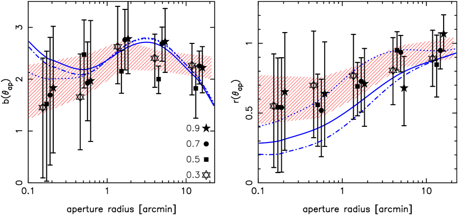
Figure 7: Relative linear stochastic bias between the red and blue galaxy sample for four mean redshifts, $b(\theta_{\rm ap})$ is in the left panel and $r(\theta_{\rm ap})$ in the right right panel. The shaded area denotes the $1\sigma$-confidence region about the mean of all redshifts taken together. The effective proper spatial scale for an aperture radius of $10^{\prime}$ at redshift $z=0.3,0.5,0.7,0.9$ is $2.8,3.8,4.5,4.8\,h^{-1}\rm Mpc$. The lines show the best-fitting models for $\bar{z}=0.7$ discussed later on in Sect. 6.3 (solid: no central galaxies, dot-dashed: red central galaxies, dotted: red and blue central galaxies). The data points are slightly shifted to increase the visibility.

4.3.2 Results

The Fig. 7 shows the inferred constraints on the relative linear stochastic bias of red and blue galaxies. Owing to relatively large remaining statistical uncertainties, which makes all redshift bins indistinguishable, we have combined the signal from all redshift bins (shaded areas).

As already seen in Fig. 6, red and blue galaxies are differently clustered with respect to the dark matter and therefore have also to be biased relative to each other. This difference is equivalent to a relative bias factor of about $b\sim 1.7-2.2$ with some evidence for a rise towards radii of about $\theta_{\rm ap}\sim 2^{\prime}$ and a subsequent decline for even smaller radii. The evidence for this scale-dependence is, however, weak. A rise is expected, though, because of the different power-law slopes of $\langle{\cal N}^{2}\rangle$ for the two samples.

For the lowest redshift bin, this is in good agreement with Madgwick et al. (2003), their Fig. 4. Furthermore, the observed scale-dependence explains why we find an overall larger value for the red/blue bias than other authors who determined the relative bias with various different methods on larger scales, e.g. Conway et al. (2005), $b\approx 1.3$ at $15\,h^{-1}\rm Mpc$, Wild et al. (2005), $b\approx 1.8$ at $10\,h^{-1}\rm Mpc$, Willmer et al. (1998), $b\approx 1.2$ at $8\,h^{-1}\rm Mpc$, Guzzo et al. (1997), $b\approx 1.7$. According to our halo model (Fig. 12), which will be discussed in the following sections, we should expect a steep decline of the bias factor down to $b\sim 1.5$ beyond our largest aperture radius which would reconcile our $b\sim 2-3$ with other studies.

Within the errors we do not see an evolution of the relative bias with redshift as, for example, has been reported by Le Fevre et al. (1996). This would support the finding of Phleps & Meisenheimer (2003).

Recently, Coil et al. (2008) have reported for DEEP2 a relative bias of $b\sim 1.28$ averaged over spatial scales between $1-15\,h^{-1}\rm Mpc$ and $b\sim 1.44$ for $0.1-15\,h^{-1}\rm Mpc$ which implies an increase of the bias for scales smaller than $1\,h^{-1}\rm Mpc$. This also agrees with our finding.

For the bias parameter $r(\theta_{\rm ap})$ we can make out a trend of decorrelation, $r\neq 1$, between the two samples towards small scales starting from about $10^{\prime}$, which corresponds to (proper) $\sim 3-5\,h^{-1}\rm Mpc$ depending on the mean redshift. We estimate that the correlation factor drops to $r\sim 0.60\pm 0.15$ on the smallest measured scale. An evolution with redshift exceeding the statistical errors is not visible.

Therefore, as other authors, we find a correlation close to unity on large scales (e.g. Wild et al., 2005; Conway et al., 2005; Blanton, 2000; Tegmark & Bromley, 1999) that is decreasing towards smaller scales. We expect our data points to become eventually consistent with $r\sim 1$ not far beyond $\theta_{\rm ap}\gtrsim 20^{\prime}$. Note, again, that we are probing smaller scales than the cited authors due to different methods.

Wang et al. (2007) studied the cross-correlation statistics of galaxy samples with different luminosities and colours in SDSS. Their results for the cross-correlation between the faint red and faint blue sample is consistent with our results. In particular, they also find a decrease of $r(\theta_{\rm ap})$ towards smaller scales (see their Fig. 16, bottom panels). Coil et al. (2008) pointed out that below a scale of $1\,h^{-1}\rm Mpc$ the cross-correlation function of their blue and red sample drops below the geometric mean of the separate auto-correlation functions. This is to say that their correlation factor becomes less than unity on these scales. In this context, see also Fig. 11 of Swanson et al. (2008) where a decorrelation towards smaller scales is found for splitting the data set into red and blue galaxies.

5 Galaxy-galaxy lensing

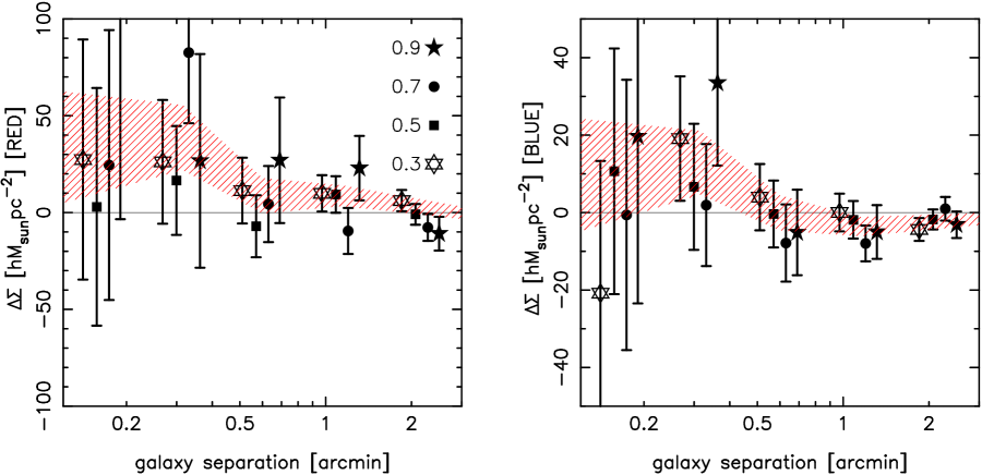
Figure 8: Differential surface mass density, $\Delta\Sigma$, as function of angular separation about lenses from the red (left panel) and blue (right panel) galaxy samples as inferred from GGL. The shaded area denotes the $1\sigma$-confidence region about the mean of all redshifts taken together. The data points are slightly shifted to increase the visibility. From the lowest to the highest redshift, a separation of $0^{\prime}\!.5$ corresponds to a projected comoving distance of $125\,h^{-1}\rm kpc$, $195\,h^{-1}\rm kpc$, $265\,h^{-1}\rm kpc$ or $320\,h^{-1}\rm kpc$, respectively.

5.1 Method

To impose further constraints on the following halo-model analysis, we additionally measure the mean tangential shear of source galaxies (GaBoDS), $\langle\gamma_{\rm t}\rangle$, as function of separation $\theta$ about the red and blue lens-galaxies (COMBO-17) for different redshifts, i.e.

$$\langle\gamma_{\rm t}(\theta)\rangle=-\big{\langle}\epsilon({\mn@boldsymbol{\theta}}_{1}){\rm e}^{-2{\rm i}\angle{\mn@boldsymbol{\theta}}_{1},{\mn@boldsymbol{\theta}}_{2}}\big{\rangle}\;,$$ (31)

where the average tangential ellipticity over all source-lens pairs with separation $\theta=|{\mn@boldsymbol{\theta}}_{1}-{\mn@boldsymbol{\theta}}_{2}|$ has to be taken (cf. Kleinheinrich et al., 2006); $\angle{\mn@boldsymbol{\theta}}_{1},{\mn@boldsymbol{\theta}}_{2}$ is the angle that is spanned by ${\mn@boldsymbol{\theta}}_{2}-{\mn@boldsymbol{\theta}}_{1}$, the difference vector between source and lens position, and the $x$-axis.

The mean tangential shear about lenses can be related to the differential projected matter over-density about lenses, in excess to the cosmic mean (e.g. McKay et al., 2001),

$$\Delta\Sigma(\theta)\equiv\overline{\Sigma}(<\theta)-\Sigma(\theta)=\frac{\langle\gamma_{\rm t}\rangle(\theta)}{\Sigma_{\rm crit}^{-1}}$$ (32)

with

$$\Sigma_{\rm crit}^{-1}=\frac{4\pi G}{c^{2}}\left\langle\frac{f_{\rm k}(w_{\rm l})f_{\rm k}(w_{\rm s}-w_{\rm l})}{f_{\rm k}(w_{\rm s})}\right\rangle\;,$$ (33)

if we specify a fiducial cosmology and the distribution of sources (lenses) in distance from the observer, $w_{\rm s}$ ($w_{\rm l}$); $\langle\ldots\rangle$ denotes the average over the lens and source distribution. The function $f_{\rm k}(w)$ is the comoving angular diameter distance as function of the comoving radial distance $w$ and the curvature, $k$, of the fiducial cosmological model. By $\overline{\Sigma}(<\theta)$ we denote the average line-of-sight over-density within a radius of $\theta$, the lens is at the disk centre, whereas $\Sigma(\theta)$ is the average over-density over an annulus with radius $\theta$. We rescale our measurements of $\langle\gamma_{\rm t}\rangle$ with $\Sigma_{\rm crit}$ in order to get rid of the influence of the lensing efficiency. This gives us comparable quantities for lenses of all redshift bins.

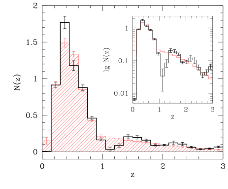
Figure 9: Distribution of sources belonging to the cosmic shear catalogue, as estimated by the photometric redshifts of galaxies inside the magnitude interval $R\in[21.5,24.5]$ in the DPS. The black histogram shows the empirical distribution, the red histogram is the fit to the data. The empirical data points around $z=1.1$ (dip) are down-weighted in the fit due to systematics in the photometric redshifts. The error bars denote the field-to-field variance. The mean redshift of the sources is $\bar{z}=0.78$. The figure is taken from Hetterscheidt et al. (2007).

For the redshift distribution of the sources we use the fit of Hetterscheidt et al. (2007) to the empirical distribution of photometric redshifts as seen in the Deep-Public Survey (DPS) (Hildebrandt et al., 2006), see Fig. 9. Our shear catalogue is a sub-sample of the shear catalogue used in that study.

A representative example for the correlation of statistical errors in the GGL estimate, and the cross-correlation between $\cal N$-statistics errors and GGL errors, is given by Fig. 5.

5.2 Results

Our measurements for of $\Delta\Sigma(\theta)$ are shown in Fig. 8. The data is binned between $6^{\prime\prime}\!\leq\theta<3^{\prime}$ into five logarithmic bins in angular separation. The remaining statistical uncertainties are high so that almost all measurements are at $1\sigma$ consistent with zero. However, when combining all redshifts bins, we find a slight signal for both the red and the blue galaxy sample. The combined red signal is higher than the blue signal, roughly by a factor of two or three. This is consistent with what was found by Kleinheinrich et al. (2006), using the same data, Sheldon et al. (2004), McKay et al. (2001) and Guzik & Seljak (2001). It implies that the environment of red galaxies (or the galaxy itself) contains more mass than the environment of a typical blue galaxy, or that the typical size of a blue lens halo is smaller than that of a red lens, although it might have the same mass than the red lens halo.

When fitting HOD parameters to the data, we use the GGL signal of the different redshift bins to constrain the allowed regime of lensing predictions by our model. Due to the large statistical uncertainties of the measurement, the GGL mainly serves as an upper limit.

6 Interpretation within a halo model framework

In this section, we translate the clustering statistics and GGL-signal of the galaxy samples into halo-model parameters. The halo-model description is utilised to describe the 3D-distribution of galaxies and dark matter. We only briefly summarise the halo-model formalism here and refer the reader to the literature for the details. How the 3D-distributions, expressed by the halo-model, relates to the observed projected angular distribution on the sky is discussed later on in Sect. 6.3. The reader may find the details on the dark matter halo properties used for this paper in Appendix A. Note that the notation used therein is introduced in this section. The Fourier transform of a function $f({\mn@boldsymbol{r}})$, denoted by a tilde $\tilde{f}({\mn@boldsymbol{k}})$, is defined in analogy to Eq. (5) but now for three dimensions.

6.1 Halo-model description

6.1.1 General halo-model formalism

The halo model is an analytical prescription for the clustering of dark matter that was motivated by N-body simulations of the cosmic structure formation (for a review: Cooray & Sheth, 2002). All matter is enclosed inside typical haloes with a given mass spectrum. Galaxy mock catalogues can be generated within this framework by populating virialised dark matter haloes with galaxies according to a prescription taken directly from semi-analytic models of galaxy formation or hydrodynamic simulation that include recipes for the formation (evolution) of galaxies (Berlind & Weinberg, 2002; Benson et al., 2000). The parameters for populating the haloes with galaxies depend solely on the halo mass. The halo-model description has been quite successful in describing or fitting observational data, although doubts about the strict validity of the basic model assumptions have been cast recently by Gao & White (2007) and Sheth & Tormen (2004) (assembly bias).

One key assumption of the halo model is that the dark matter density or galaxy number density are linear superpositions of in total $N_{\rm h}$ haloes with a typical radial profile:

$$n_{i}({\mn@boldsymbol{r}})=\sum_{j=1}^{N_{\rm h}}N_{i}(m_{j})u_{i}({\mn@boldsymbol{r}}-{\mn@boldsymbol{r}}_{j},m_{j})\;.$$ (35)

The halo profiles, $u_{i}$, describe the spatial distribution of galaxies, $i>0$, or dark matter, $i=0$, within haloes. All profiles considered here are normalised to unity.

The profiles depend on an additional parameter, $m$, which is the total mass of the dark matter halo, ${\mn@boldsymbol{r}}$ is a position within the comoving frame and ${\mn@boldsymbol{r}}_{i}$ is the centre of the $i$-th halo. By $N_{i}(m_{j})$ we denote either the number of galaxies, type $i$, populating the $j$-th halo (if $i>0$), or if $i=0$ the dark matter mass, $m_{j}$, that is attached to the $j$-th halo. In the latter case, $n_{0}({\mn@boldsymbol{r}})$ is simply the dark matter density as function of position. In particular, $N_{0}$ and $N_{i}$ with $i>0$ have, for convenience within the formalism, different units (halo mass versus number of galaxies).

In general, the halo-occupation number $N_{i}(m_{j})$ and the halo centre, ${\mn@boldsymbol{r}}_{j}$, are random numbers. The conditional probability distribution of the halo-occupation number, $P(N_{i}|m_{j})$, is a function of the halo mass only. In the case of dark matter, $i=0$, one has simply $N_{0}(m_{j})\equiv m_{j}$, i.e. $P(N_{0}|m_{j})=\delta_{\rm D}(N_{0}-m_{j})$, thus the mass associated with a “dark matter halo $m_{i}$” is always $m_{i}$, whereas the number of galaxies living inside haloes of same mass may vary from halo to halo.

Both $N_{i}(m_{j})$ and $u_{i}({\mn@boldsymbol{r}},m_{j})$ depend solely on $m_{j}$ and not on the mass or position of any other halo. Moreover, the position of a halo, ${\mn@boldsymbol{r}}_{j}$, and its mass, $m_{j}$, are postulated to be statistically independent. However, the halo-occupation numbers of different galaxies $i$ and $j$ inside the same halo may be statistically dependent on each other. For example, inside the same halo the number of red galaxies may be related to the number of blue galaxies and vice versa. This is the idea behind the concept of the joint halo-occupation distribution.

Based on these assumptions, the halo model predicts the 3D-power spectra of galaxy number density correlations, galaxy-mass density correlations and mass-mass correlations, $P_{ij}(k)$, as function of a halo mass spectrum, halo bias parameters, typical density profiles and a HOD of galaxies:

$$\frac{\big{\langle}\tilde{n}_{i}({\mn@boldsymbol{k}})\tilde{n}_{j}({\mn@boldsymbol{k}}^{\prime})\big{\rangle}}{\bar{n}_{i}\bar{n}_{j}}=(2\pi)^{3}P_{ij}(|{\mn@boldsymbol{k}}|)\delta_{\rm D}({\mn@boldsymbol{k}}+{\mn@boldsymbol{k}}^{\prime})\;.$$ (36)

Here and in the following, $\langle\ldots\rangle$ is the statistical average over all possible haloes, and $\bar{n}_{i}$ means the average number of galaxies per unit volume. This paper only considers isotropic halo density profiles $u_{i}({\mn@boldsymbol{r}},m)$ independent of the direction of ${\mn@boldsymbol{r}}$, so that:

$$\tilde{u}_{i}(k,m)=\frac{\int_{0}^{\infty}{\rm d}r\,rk^{-1}\,u_{i}(r,m)\sin{(kr)}}{\int_{0}^{\infty}{\rm d}r\,r^{2}\,u_{i}(r,m)}\;.$$ (37)

This equation includes a normalisation of the density profile.

Following the calculations of Scherrer & Bertschinger (1991) one finds for the power spectra ($k>0$ and $N_{\rm h}\gg 1$):

$$P_{ij}(k)=P_{ij}^{\rm 1h}(k)+P_{ij}^{\rm 2h}(k)\;,$$ (38)

where the so-called one-halo term is

$$P_{ij}^{\rm 1h}(k)=\frac{\overline{m}}{\bar{\rho}\overline{N}_{i}\overline{N}_{j}}\int_{0}^{\infty}\!\!\!\!\!\!{\rm d}m\,n(m)K^{\rm 1h}_{ij}(k,m)\;,$$ (39)

the two-halo term

$$P_{ij}^{\rm 2h}(k) = \frac{1}{\overline{N}_{i}\overline{N}_{j}}\int_{0}^{\infty}\!\!\!{\rm d}m_{1}\,n(m_{1})\int_{0}^{\infty}\!\!\!{\rm d}m_{2}\,n(m_{2})\times$$

$$P(k,m_{1},m_{2})K^{\rm 2h}_{ij}(k,m_{1},m_{2})$$

and

$$\overline{N}_{i}=\int_{0}^{\infty}{\rm d}m\,n(m)\,\big{\langle}N_{i}(m)\big{\rangle}~{};~{}\overline{m}=\int_{0}^{\infty}{\rm d}m\,n(m)\,m\;.$$ (41)

The mean number density of galaxies is

$$\bar{n}_{i}=\big{\langle}n_{i}({\mn@boldsymbol{r}})\big{\rangle}=\frac{\bar{\rho}}{\overline{m}}\,\overline{N}_{i}\;.$$ (42)

The function $n(m){\rm d}m$ is usually the mean number density of haloes within the mass interval $[m,m+{\rm d}m]$. Note, however, that in the above equations, and for the following $\bar{n}_{i}$, $n(m)$ may be rescaled by any arbitrary constant without changing the results. The average $\big{\langle}N_{i}(m)\big{\rangle}$ is the mean number of galaxies found within a halo of mass $m$ (for $i>0$), or the mass of the halo itself, if $i=0$. Notice that after the statistical average performed for the power spectra we have shifted the notation from $N_{i}(m_{k})$ (number of $i$-galaxies inside halo $k$) to $N_{i}(m)$ (number of $i$-galaxies inside a halo of mass $m$).

By $\bar{\rho}=\rho_{\rm crit}\Omega_{\rm m}$ we denote the mean comoving matter density of the dark matter that is included inside the dark matter haloes. The constant $\Omega_{\rm m}$ is the matter density parameter and $\rho_{\rm crit}$ the critical density.

The different cases of power spectra (galaxy auto-power spectra, galaxy cross-power spectra, dark matter/galaxy cross-power spectra) give different results for the above integrals. To save space, all variants are encapsulated into the integral kernels

$$K^{\rm 1h}_{ij}(k,m) = \big{\langle}\sum_{q=1}^{N_{i}(m)}\tilde{u}^{(q)}_{i}(k,m)\sum_{r=1}^{N_{j}(m)}\tilde{u}^{(r)}_{j}(k,m)\big{\rangle}-$$

$$-\delta^{\rm K}_{ij}\big{\langle}\sum_{q=1}^{N_{j}(m)}[\tilde{u}^{(q)}_{j}(k,m)]^{2}\big{\rangle}\;,$$

$$K^{\rm 2h}_{ij}(k,m) = \big{\langle}\sum_{q=1}^{N_{i}(m)}\tilde{u}^{(q)}_{i}(k,m)\big{\rangle}\big{\langle}\sum_{r=1}^{N_{j}(m)}\tilde{u}^{(r)}_{j}(k,m)\big{\rangle}\;,$$ (44)

where $\langle\ldots\rangle$ denotes the average over all haloes of mass $m$ and $\tilde{u}_{i}^{(q)}(k,m)$ expresses the spatial probability distribution of the $q$-th, out of $q\in[1,N_{i}(m)]$, galaxies belonging to the sample $i$ and a particular halo of mass $m$.

We need this further distinction into various spatial distributions since we may split a galaxy sample into one central galaxy – sitting at the halo centre hence having $\tilde{u}(k,m)=1$ – and $(N_{i}(m)-1)$ satellite galaxies with a different distribution. The term with the Kronecker pre-factor, $\delta^{\rm K}_{ij}$, in Eq. (6.1.1) is only applied if both samples $i$ and $j$ are discrete (galaxies). It accounts for the subtraction of white shot-noise contribution, $1/\bar{n}_{i}$, to the clustering power that is not measured due to the definition of the clustering correlation function, $\omega(\theta)$ (excess of pairs over a uniform distribution), and the aperture statistics. For the smooth dark matter, $i=0$, one has to substitute in the Eqs. (6.1.1) and (44) $\sum_{q=1}^{N_{i}(m)}\tilde{u}^{(q)}_{i}(k,m)\equiv m\,\tilde{u}_{0}(k,m)$, which simplifies the equations.

As an example, if all galaxies of a same sample $i$ have identical spatial distributions, $\tilde{u}_{i}(k,m)$, one will find for $i\neq j$ and $i,j>0$:

$$\sum_{q=1}^{N_{i}(m)}\tilde{u}_{i}^{(q)}(k,m) = \!\!N_{i}(m)\tilde{u}_{i}(k,m)\;,$$ (45)

$$K^{\rm 1h}_{ij}(k,m)\!\!\! = \tilde{u}_{i}(k,m)\tilde{u}_{j}(k,m)\big{\langle}N_{i}(m)N_{j}(m)\big{\rangle}\;,$$

$$K^{\rm 2h}_{ij}(k,m)\!\!\! = \tilde{u}_{i}(k,m)\tilde{u}_{j}(k,m)\big{\langle}N_{i}(m)\big{\rangle}\big{\langle}N_{j}(m)\big{\rangle}\;.$$

A galaxy sample with $N_{i}^{\rm cen}(m)\in\{0,1\}$ central galaxies and $N_{i}^{\rm sat}(m)$ satellites of same in-halo distribution $\tilde{u}_{i}(k,m)$ has

$$\sum_{q=1}^{N_{i}(m)}\tilde{u}_{i}^{(q)}(k,m)=N_{i}^{\rm cen}(m)+N^{\rm sat}_{i}(m)\tilde{u}_{i}(k,m)\;.$$ (46)

From Eq. (45) and (46) all kernels relevant for this paper follow. They are listed in Table 3.

Table 3: Integration kernels for the one- and two-halo term, Eqs. (39) and (6.1.1). In the simple model, all galaxies of same type are distributed over the halo the same way. For the central-galaxy scenario, the halo occupation, $N_{i}(m)=N_{i}^{\rm cen}(m)+N_{i}^{\rm sat}(m)$, of every galaxy type, $i$, is split into a central galaxy and satellite galaxies. Here, it is explicitly assumed that $N_{i}^{\rm sat}(m)>0$ requires $N_{i}^{\rm cen}(m)=1$, i.e. $\langle N_{i}^{\rm cen}(m)N_{i}^{\rm sat}(m)\rangle=\langle N_{i}^{\rm sat}(m)\rangle$. The mixed model assumes one type of galaxies, $i$, to possess a central galaxy and another, $j$, having no central galaxy as in the simple model. For that case, $i$ is described by the central model, $j$ by the simple model; only for the cross-correlation of both a new kernel is needed. Note that $N_{0}(m)\equiv m$, dark matter is always “simple”.

$i$	$j$		integral kernel $K_{ij}^{\rm 1h}(k,m)$	model type
$0$	$0$		$[\tilde{u}_{0}(k,m)]^{2}m^{2}$	simple
				.
$i>0$	$j=i$		$[\tilde{u}_{i}(k,m)]^{2}\big{\langle}N_{i}(m)\left(N_{i}(m)-1\right)\big{\rangle}$	.
				.
$i>0$	$j\neq i$		$\tilde{u}_{i}(k,m)\tilde{u}_{j}(k,m)\big{\langle}N_{i}(m)N_{j}(m)\big{\rangle}$	.
$i>0$	$0$		$\tilde{u}_{0}(k,m)m\big{\langle}N_{i}^{\rm cen}(m)\big{\rangle}+\tilde{u}_{i}(k,m)\tilde{u}_{0}(k,m)m\big{\langle}N_{i}^{\rm sat}(m)\big{\rangle}$	central
				.
$i>0$	$j=i$		$2\tilde{u}_{i}(k,m)\big{\langle}N_{i}^{\rm sat}(m)\big{\rangle}+[\tilde{u}_{i}(k,m)]^{2}\big{\langle}N_{i}^{\rm sat}(m)\left(N_{i}^{\rm sat}(m)-1\right)\big{\rangle}$	.
				.
$i>0$	$j\neq i>0$		$\tilde{u}_{i}(k,m)\big{\langle}N_{i}^{\rm sat}(m)N_{j}^{\rm cen}(m)\big{\rangle}+\tilde{u}_{j}(k,m)\big{\langle}N_{j}^{\rm sat}(m)N_{i}^{\rm cen}(m)\big{\rangle}+$	.
				.
			$\tilde{u}_{i}(k,m)\tilde{u}_{j}(k,m)\big{\langle}N_{i}^{\rm sat}(m)N_{j}^{\rm sat}(m)\big{\rangle}+\big{\langle}N_{i}^{\rm cen}(m)N_{j}^{\rm cen}(m)\big{\rangle}$	.
$i>0$	$j\neq i$		$\tilde{u}_{j}(k,m)\big{\langle}N_{i}^{\rm cen}(m)N_{j}(m)\big{\rangle}+\tilde{u}_{i}(k,m)\tilde{u}_{j}(k,m)\big{\langle}N_{i}^{\rm sat}(m)N_{j}(m)\big{\rangle}$	mixed
$i$	$j$		integral kernel $K_{ij}^{\rm 2h}(k,m_{1},m_{2})$	model type
$i$	$j$		$\tilde{u}_{i}(k,m_{1})\tilde{u}_{j}(k,m_{2})\big{\langle}N_{i}(m_{1})\big{\rangle}\big{\langle}N_{j}(m_{2})\big{\rangle}$	simple
$i>0$	$0$		$\tilde{u}_{0}(k,m_{2})m_{2}\left[\big{\langle}N_{i}^{\rm cen}(m_{1})\big{\rangle}+\tilde{u}_{i}(k,m_{1})\big{\langle}N_{i}^{\rm sat}(m_{1})\big{\rangle}\right]$	central
				.
$i>0$	$j>0$		$\left[\tilde{u}_{j}(k,m_{1})\big{\langle}N_{i}^{\rm cen}(m_{1})\big{\rangle}+\tilde{u}_{i}(k,m_{1})\tilde{u}_{j}(k,m_{1})\big{\langle}N_{i}^{\rm sat}(m_{1})\big{\rangle}\right]\times$	.
				.
			$\left[\tilde{u}_{i}(k,m_{2})\big{\langle}N_{j}^{\rm cen}(m_{2})\big{\rangle}+\tilde{u}_{i}(k,m_{2})\tilde{u}_{j}(k,m_{2})\big{\langle}N_{j}^{\rm sat}(m_{2})\big{\rangle}\right]$	.
$i>0$	$j\neq i$		$\tilde{u}_{j}(k,m_{2})\big{\langle}N_{j}(m_{2})\big{\rangle}\left[\big{\langle}N_{i}^{\rm cen}(m_{1})\big{\rangle}+\tilde{u}_{i}(k,m_{1})\big{\langle}N_{i}^{\rm sat}(m_{1})\big{\rangle}\right]$	mixed

The function $P(k,m_{1},m_{2})$ means the cross-power spectrum of the number densities of haloes with masses $m_{1}$ and $m_{2}$. It is common practice to assume a linear deterministic biasing between the halo number density and the linear dark matter density (Cooray & Sheth, 2002):

$$P(k,m_{1},m_{2})\approx P_{\rm lin}(k)\,b(m_{1})\,b(m_{2})$$ (47)

with $b(m)$ being the linear bias factor of haloes with mass $m$ and $P_{\rm lin}(k)$ the linear dark matter power spectrum. This reduces the 2D-integral in Eq. (6.1.1) to a simpler product of 1D-integrals.

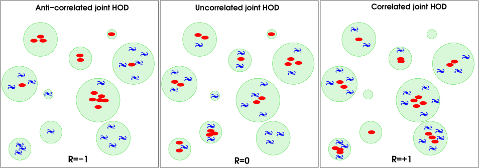
Figure 10: Simplified illustration of the concept of the joint halo occupation distribution for three cases. Left panel: the dark matter haloes (shady disks) are filled with different galaxy types that tend to avoid each other. If the number of red, elliptical, galaxies is increased for a halo of given size, the number of blue spiral, galaxies decreases. Right panel: over- and under densities of the two galaxy populations are highly correlated. If the number of red galaxies for a halo of a given size increases, the number of blue galaxies increases as well. Middle panel: the halo-occupation numbers are not correlated.

6.1.2 Joint halo-occupation distribution

Within the framework of the halo model (see Eqs. (39) and (6.1.1)), one works out the clustering statistics of galaxies by specifying the mean number of galaxies for a halo of certain mass $m$, $\langle N_{i}(m)\rangle$, and the mean number of galaxy pairs, either pairs of the same galaxy type (auto-power), $\langle N_{i}(m)(N_{i}(m)-1)\rangle$, or pairs between different galaxy types (cross-power), $\langle N_{i}(m)N_{j}(m)\rangle$. Things become slightly more difficult, though, if we distinguish between central galaxies and satellite galaxies as can be seen in Table 3.

In general, the number of galaxies or galaxy pairs for a fixed halo mass are first and $2^{\rm nd}$-order moments of a joint halo occupation distribution (JHOD) of two galaxy populations $i$ and $j$. The JHOD, $P(N_{i},N_{j}|m)$, determines the probability to find a certain number of “galaxies $i$” and “galaxies $j$” inside the same halo of mass $m$. The $2^{\rm nd}$-order moment,

$$\langle N_{i}(m)N_{j}(m)\rangle=\sum_{N_{i},N_{j}=0}^{\infty}P(N_{i},N_{j}|m)\,N_{i}N_{j}\;,$$ (48)

of the JHOD can conveniently be parameterised in terms of the mean halo-occupation number,

$$\big{\langle}N_{i}(m)\big{\rangle}=\sum_{N_{i},N_{j}=0}^{\infty}P(N_{i},N_{j}|m)\,N_{i}\;,$$ (49)

the (central) variance of the HOD,

$$\sigma_{i}(m)\equiv\sqrt{\big{\langle}N^{2}_{i}(m)\big{\rangle}-\big{\langle}N_{i}(m)\big{\rangle}^{2}}\;,$$ (50)

and the JHOD-correlation factor:

$$R_{ij}(m)\equiv\frac{\big{\langle}N_{i}(m)N_{j}(m)\big{\rangle}-\big{\langle}N_{i}(m)\big{\rangle}\big{\langle}N_{j}(m)\big{\rangle}}{\sigma_{i}(m)\sigma_{j}(m)}\;.$$ (51)

The JHOD correlation factor expresses the tendency of two populations to avoid or attract each other inside the same halo. See Fig. 10 for a simplified illustration. This tendency, however, can only be seen in the one-halo term of the cross-power spectrum, Eq. (39), which is observable when considering the cross-power (cross-correlation function) of two galaxy populations for small separations.

The effect of the JHOD correlation factor $R_{ij}(m)$ on the cross-moments becomes negligible, i.e.

$$\big{\langle}N_{i}(m)N_{j}(m)\big{\rangle}\approx\big{\langle}N_{i}(m)\big{\rangle}\big{\langle}N_{j}(m)\big{\rangle}\;,$$ (52)

if the relative fluctuations in galaxy numbers inside haloes become small, i.e. if $\sigma_{i}(m)/\big{\langle}N_{i}(m)\big{\rangle}\ll 1$. Since haloes with mean galaxy occupation numbers of more than roughly one are expected to have a Poisson variance, one can expect that the JHOD correlation factor loses significance for massive haloes. For large $m$ the relative variance becomes $\propto 1/\sqrt{\langle N_{i}(m)\rangle}$.

In order to avoid confusion, we would like to stress again that $R_{ij}$ expresses the correlation of galaxy numbers inside single haloes, whereas $r(\theta_{\rm ap})$ is a correlation of galaxy number densities as seen in the angular clustering of galaxies.

6.2 Adopted model for JHOD of red and blue galaxies

In the following we describe the details of the HOD of the red and blue galaxy sample. A galaxy sample (blue or red) can either have a central galaxy and satellites or solely consists of satellites. Satellites are distributed according to the dark matter in a halo, but possibly with a different concentration parameters. Central galaxies sit at or close to the centre of a halo, for the latter of which our “central models” are an approximation. We will distinguish three different model flavours:

1. A scenario in which we have only red and blue satellites populating a dark matter halo.

2. A scenario in which red galaxies are both central and satellite galaxies, blue galaxies are only satellites.

3. A scenario in which we have red and blue central galaxies and red and blue satellites.

Case ii) is motivated by the observation that galaxy clusters often have red galaxies as central galaxies. Case iii) is motivated by the possibility that the observed galaxy-galaxy lensing signal of the blue galaxies and the power-law clustering may also require a central blue galaxy.

We start off with the description of the HOD of a single sample. The interconnection of the red and blue sample is discussed later on where we address the problem of red/blue galaxy pairs.

For modelling the HOD of our red and blue galaxy sample we use, with some minor modifications, the parametrisations that were discussed in Zheng et al. (2007), Zheng & Weinberg (2007) and Zheng et al. (2005).

6.2.1 Mean galaxy numbers and distribution inside haloes

The HOD (red and blue) for haloes with mass $m$,

$$N(m)=N^{\rm cen}(m)+N^{\rm sat}(m)\;,$$ (53)

is split into one central galaxy, $N^{\rm cen}(m)\in\{0,1\}$, and satellite galaxies, $N^{\rm sat}(m)$. A central galaxy is placed at the centre of the halo. If there is a galaxy inhabiting a halo, there is always one central galaxy. This is used in the following relations. Satellite galaxies are distributed according to a NFW profile with concentration parameter $c^{\prime}=fc$, where $c$ is the concentration of the dark matter (Appendix A). For $f>1$ galaxies populating the haloes are more concentrated than the dark matter, while for $f<1$ galaxies are less concentrated than the dark matter.

The halo mass dependence of the mean HOD is assumed to be

$$\big{\langle}N(m)\big{\rangle} = \big{\langle}N^{\rm cen}(m)\big{\rangle}+\big{\langle}N^{\rm sat}(m)\big{\rangle}\;,$$ (54)

$$\big{\langle}N^{\rm cen}(m)\big{\rangle} = \frac{1}{2}\left[1+{\rm erf}{\left(\frac{\log{m}-\log{m_{\rm min}}}{\sigma_{\log{m}}}\right)}\right]\;,$$ (55)

$$\big{\langle}N^{\rm sat}(m)\big{\rangle} = \big{\langle}N^{\rm cen}(m)\big{\rangle}\left(\frac{m-m_{0}}{m^{\prime}}\right)^{\epsilon}{\rm H}(m-m_{0})\;,$$ (56)

where

$${\rm erf}(x)=\frac{2}{\sqrt{\pi}}\int_{0}^{x}{\rm d}t\,{\rm e}^{-t^{2}}$$ (57)

is the error function.

We would like to keep the number of parameters, required to explain the data, as small as possible. For that reason, we set $m_{0}=m_{\rm min}$ because we found that a free $m_{\rm min}$ does not significantly improve our fits. An additional parameter $f\neq 1$, on the other hand, that gives some freedom in the shape of the density profiles of blue and red galaxies yields improved fits and is therefore included.

Note that due to the previous definition of $\langle N(m)\rangle$ we can still have (central) galaxies for $m\leq m_{\rm min}$, as $1+{\rm erf}(x)\neq 0$ for $x<0$. Other authors prefer to define a hard cut-off for $N(m)$, as for instance in Phleps et al. (2006).

6.2.2 Number of galaxy pairs of same sample

In the original model, the fluctuation in the number of satellites is assumed to be Poisson (referred to as “Poisson satellite” model hereafter; Kravtsov et al., 2004), i.e. $\langle[N^{\rm sat}]^{2}\rangle=\langle N^{\rm sat}\rangle^{2}+\langle N^{\rm sat}\rangle$. Their assumption completely fixes the variance of the total number of galaxies inside a halo to (we skip in the following the arguments “$(m)$” to save space):

$$\sigma^{2}(N)\!\!\! = \langle N^{2}\rangle-\langle N\rangle^{2}$$

$$= \langle N(N-1)\rangle+\langle N\rangle(1-\langle N\rangle)$$

$$= 3\langle N^{\rm sat}\rangle+\langle N^{\rm cen}\rangle\left(1-2\langle N^{\rm sat}\rangle\right)-\langle N^{\rm cen}\rangle^{2}\;,$$

because the variance of the number of central galaxies is always

$$\sigma^{2}(N^{\rm cen})=\langle N^{\rm cen}\rangle[1-\langle N^{\rm cen}\rangle]\;,$$ (59)

owing to the fact that $N^{\rm cen}$ is only zero or one (Bernoulli distribution). In particular we have $\langle[N^{\rm cen}]^{2}\rangle=\langle N^{\rm cen}\rangle$.

The HOD variance or number of galaxy pairs of the “Poisson satellite” model can, using the notation of Scoccimarro et al. (2001), be written as

$$\langle N(N-1)\rangle=\alpha^{2}\langle N\rangle^{2}~{}\;;~{}\alpha^{2}\equiv\frac{\langle N^{\rm sat}\rangle(\langle N^{\rm sat}\rangle+2)}{(\langle N^{\rm cen}\rangle+\langle N^{\rm sat}\rangle)^{2}}\;,$$ (60)

where $\langle N(N-1)\rangle$ is the mean number of galaxy pairs, regardless of whether they are central galaxies or satellites. The variance (or number of galaxy pairs, see Eq. (6.2.2)) becomes Poisson for haloes $m$ with $\alpha=1$, sub-Poisson for $\alpha<1$ and super-Poisson for $\alpha>1$. In the “Poisson satellite” model $\alpha$ is a function increasing slowly from zero near $m=m_{\rm min}$ to unity for large $\langle N(m)\rangle$. See the dashed line in right panel of Fig. 11.

We found, however, that this mean number of galaxy pairs per halo hardly reproduces the deep decrease in the bias parameter $r(\theta_{\rm ap})$ of our red and blue galaxy sample (see Section 4.3), presumably because it becomes Poisson at too large $m$.

For that reason, we relax the assumption of the “Poisson satellite” model by introducing another model parameter, $\lambda$, that delays the onset of a Poisson variance in $N(m)$, $\lambda<1$, or accelerates it, $\lambda>1$. We achieve this by keeping the shape of $\alpha(m)$ as in the “Poisson satellite” model, Eq. (60), but rescaling the (log)mass scale, giving us a new $\alpha^{\prime}(m)$:

$$\alpha^{\prime}(m)\equiv\alpha\!\left(m\times[m/m_{\rm min}]^{\lambda-1}\right)\;.$$ (61)

Thus, for $\lambda=1$ our model uses exactly the same HOD variance that is postulated in the original satellite model. Compare this to the parametrisation of Scoccimarro et al. (2001), where $\alpha(m)$ is postulated to increase linearly with $\ln{m}$ from $m_{\rm min}$ onwards.

The number of satellite pairs, needed for the power spectra integrals, is then calculated from $\alpha^{\prime}(m)$ via

$$\langle N^{\rm sat}(N^{\rm sat}-1)\rangle=[\alpha^{\prime}]^{2}\langle N\rangle^{2}-2\langle N^{\rm sat}\rangle\;,$$ (62)

invoking the relation between $\alpha(m)$, now substituted by the rescaled $\alpha^{\prime}(m)$, and the mean number of galaxy pairs. Following from this, the variance of the number of satellites is consequently

$$\sigma^{2}(N^{\rm sat})=[\alpha^{\prime}]^{2}\langle N\rangle^{2}-\langle N^{\rm sat}\rangle(\langle N^{\rm sat}\rangle+1)\;.$$ (63)

The variance of the total number of galaxies, required for models lacking central galaxies, is simply

$$\sigma^{2}(N)=[\alpha^{\prime}]^{2}\langle N\rangle^{2}+\langle N\rangle(1-\langle N\rangle)\;.$$ (64)

The variance parameter $\alpha(m)$ cannot be reduced arbitrarily, though, as a too small variance (too sub-Poisson) may be in conflict with the mean number of galaxies. Put in other words, the number of pairs, Eqs. (60) and (62), and the variances, Eqs. (63) and (64), have to be larger or equal than zero, i.e.

$$[\alpha^{\prime}]^{2}\geq{\rm max}\!\left\{\frac{2\langle N^{\rm sat}\rangle}{\langle N\rangle^{2}},\frac{\langle N^{\rm sat}\rangle(1+\langle N^{\rm sat}\rangle)}{\langle N\rangle^{2}},1-\frac{1}{\langle N\rangle}\right\}\;.$$ (65)

If $[\alpha^{\prime}]^{2}$ is smaller than the r.h.s., we set $[\alpha^{\prime}]^{2}$ equal to the r.h.s. As $\alpha^{\prime}$ is usually an increasing function with halo mass $m$, this resetting is not necessary for $\lambda\geq 1$ but may be important if we try to delay Poisson statistics compared to the “Poisson satellite” model.

Figure 11: Effect of the HOD variance parameter $\lambda$ (for both populations equally) on the cross-correlation function of two hypothetical populations of galaxies. The parameters for the galaxy populations were chosen arbitrarily from Zheng et al. (2005). As model parameters red galaxies have $\{10^{12.69}{\rm M}_{\odot},0.15,10^{12.94}{\rm M}_{\odot},10^{13.82}{\rm M}_{\odot},1.08\}$, blue galaxies have $\{10^{11.68}{\rm M}_{\odot},0.15,10^{11.86}{\rm M}_{\odot},10^{13}{\rm M}_{\odot},1.02\}$ for $\{m_{\rm min},\sigma_{\log{m}},m_{0},m^{\prime},\epsilon\}$ (see text for details). The galaxy concentration is set $f=1$ in both cases, both populations have no central galaxy component. The JHOD correlation factor is set to $R=+1$. Galaxies are uniformly distributed within the redshift range $z\in[0.2,0.4]$. Left panel: Different lines correspond to a bias parameter $r(\theta_{\rm ap})$ for different $\lambda$ (numbers attached to solid lines). Top line: a variance of the HOD according to the “Poisson satellite” model, $\lambda=1$. Bottom line: a variance almost Poisson for all haloes, $\lambda=10$. Right panel: The corresponding HOD variance parameter, $[\alpha^{\prime}(m)]^{2}$, of the blue galaxies for some of the lines in the left panel.

The effect of $\lambda$ on the bias parameter $r(\theta_{\rm ap})$ is demonstrated in Fig. 11 for some particular examples. It is remarkable to see that an early (low $m$) Poisson variance in the galaxy number suppresses the cross-power towards smaller $r(\theta_{\rm ap})\lesssim 1$, while a late Poisson variance (higher $m$) yields higher values for $r(\theta_{\rm ap})\gtrsim 1$ on small scales. Therefore, the bias parameter $r(\theta_{\rm ap})$ promises to be a probe for the variance in the HOD.

Finally, with this parametrisation each galaxy sample has six, $\{m_{\rm min},\sigma_{\log{m}},m^{\prime},\epsilon,f,\lambda\}$, different parameters. Moreover, we have one more additional parameter which expresses the correlation within the JHOD of blue and red galaxies.

Based on this, we consider three different flavours of the model – detailed in the following sections – which permit red or/and blue galaxies as central galaxies and always have red and blue satellites. If a sample has no central galaxy, we still use $\langle N(m)\rangle$ as in Eq. (54) and $\langle N(N-1)\rangle$ as in Eq. (60) (with rescaled $\alpha$) but distribute all $N(m)$ galaxies like “satellites” over the halo; $\langle N(m)\rangle$ is the HOD of all galaxies in that case. This tests the idea – no central galaxy for a galaxy population but everything else in the model unchanged – if the data really requires a galaxy sample to have a central galaxy.

Figure 12: Example predictions for the relative linear stochastic bias of red and blue galaxies for three different scenarios (with/without central galaxy component, only red galaxies have a central component). The model parameters are chosen as in Fig. 11 except that we fix $\lambda=3.0$ for both blue and red galaxies and we vary the JHOD parameter $R$. Left figure: The bias parameter $r(\theta_{\rm ap})$ is plotted (solid lines) for two different JHOD-correlation factors (halo-mass invariant), $R=\pm 1$. To separate contributions to the cross-power originating from the one-halo (1h; dashed line) and two-halo (2h; dotted line) term, the cross-power was recalculated for $R=+1$ considering only one contribution at a time. The solid thick line in the right panel assumes a model where the blue and red samples have a central component, whereas the thick dashed-dotted line is for a model where only the red sample has a central component (no one-halo/two-halo term splitting). Right figure: Linear bias factor, $b(\theta_{\rm ap})$ (solid lines; red galaxies are more strongly clustered). The JHOD-correlation factor has no impact here. To estimate the importance of the one- and two-halo terms, $b(\theta_{\rm ap})$ was also recalculated with the red galaxy power spectrum consisting of only either the one- or two-halo term. The thick dashed-dotted line in the right panel corresponds to the model where only the red sample has a central component(no one-halo/two-halo term splitting).

In Fig. 12 we show a few examples for the linear stochastic bias between two galaxy populations based on the three scenarios, detailed below. By splitting the contributions to the cross-power spectrum, stemming from the one- and two-halo terms, the figure shows in which regime we can expect the two different terms to dominate. The transition is roughly at an aperture radius of $20\,\rm arcmin$ for a mean redshift of $z\sim 0.3$. This corresponds to an effective projected (proper) scale of $5.6\,h^{-1}\rm Mpc$. For comparison, the (comoving) virial radius of a NFW halo with $m\approx 1.4\times 10^{14}\,h^{-1}{\rm M}_{\odot}$ is $r_{\rm vir}\approx 0.8\,h^{-1}\rm Mpc$, or $r_{\rm vir}\approx 0.64\,h^{-1}{\rm Mpc}\,\,(m/10^{14}\,h^{-1}{\rm M}_{\odot})^{0.33}$. Also shown is the clear impact of the JHOD correlation factor. Galaxies with tendency of avoidance have a smaller cross-power.

6.2.3 Number of cross-pairs for red and blue central galaxies

The statistical cross-moments for a central galaxy scenario (central galaxies for both or just one population) requires generally more information on the JHOD than just first- and $2^{\rm nd}$-order moments of $P(N_{i},N_{j}|m)$. The correlations between satellite numbers and central galaxy numbers have to be specified as well. Namely, required are also $\langle N_{i}(m)|N_{j}(m)=0\rangle$, the mean number of $i$-galaxies for haloes which do not contain any $j$-galaxy, and $P(N_{i}(m)N_{j}(m)=0)$, which is the probability to find either no $i$-galaxy or no $j$-galaxy inside a halo of mass $m$. We show this in Appendix B.

To not unnecessarily increase the number of free model parameters in a central-satellite galaxy scenario, we can make a reasonable approximation, though. For every galaxy population having central galaxies, we set $N^{\rm cen}=1$ for halo masses $m$ where the mean number of galaxies is $\langle N(m)\rangle\geq 1$, and $N^{\rm sat}=0$ otherwise. This means that if the mean number of galaxies belonging to a population is less or equal one, it is essentially only the central galaxy we can find in those haloes. On the other hand, if the mean galaxy number is larger than one, then there is always at least a central galaxy.

Applying this approximation allows us to express the cross-moments of the HOD entirely in terms of known variances, means and the JHOD correlation factor $R_{ij}(m)$. In a scenario with blue and red central galaxies, we hence distinguish four cases:

1. Case: $\langle N_{i}\rangle<1$, $\langle N_{j}\rangle<1$
   Here, we have

   $$\langle N_{i}^{\rm sat}N_{j}^{\rm cen}\rangle = \langle N_{j}^{\rm sat}N_{i}^{\rm cen}\rangle=\langle N_{i}^{\rm sat}N_{j}^{\rm sat}\rangle=0\;.$$ (66)

2. Case: $\langle N_{i}\rangle\geq 1$, $\langle N_{j}\rangle<1$
   We will use:

   $$\big{\langle}N^{\rm sat}_{i}N^{\rm sat}_{j}\big{\rangle} = \big{\langle}N^{\rm cen}_{i}N^{\rm sat}_{j}\big{\rangle}=0\;,$$ (67)

   $$\big{\langle}N^{\rm sat}_{i}N^{\rm cen}_{j}\big{\rangle} = \!\!\big{\langle}N^{\rm sat}_{i}\big{\rangle}\big{\langle}N^{\rm cen}_{j}\big{\rangle}+R_{ij}\sigma(N_{i}^{\rm sat})\sigma(N_{j}^{\rm cen})\;.$$

3. Case: $\langle N_{i}\rangle\geq 1$, $\langle N_{j}\rangle\geq 1$
   Finally for richly populated haloes, we will have:

   $$\big{\langle}N^{\rm cen}_{i}N^{\rm sat}_{j}\big{\rangle} = \big{\langle}N^{\rm sat}_{j}\big{\rangle}~{}\;;~{}\big{\langle}N^{\rm sat}_{i}N^{\rm cen}_{j}\big{\rangle}=\big{\langle}N^{\rm sat}_{i}\big{\rangle}\;,$$ (68)

   $$\big{\langle}N^{\rm sat}_{i}N^{\rm sat}_{j}\big{\rangle} = \!\!\big{\langle}N^{\rm sat}_{i}\big{\rangle}\big{\langle}N^{\rm sat}_{j}\big{\rangle}+R_{ij}\sigma(N_{i}^{\rm sat})\sigma(N_{j}^{\rm sat})\;.$$

For the sake of simplicity, this model unrealistically also assumes that red and blue galaxies have central galaxies simultaneously, which would mean for haloes hosting red and blue galaxies that we would find a red and blue galaxy at, or very close, to the centre. A more realistic model would add another rule that decides when (and with what probability) we have a red or a blue central galaxy, but never both at the same time.

However, our approximation is fair as long as we rarely find haloes with one red and one blue galaxies. As seen later on, our galaxy samples start to populate haloes at different mass-thresholds, blue galaxies from $\sim 10^{11}{\rm M}_{\odot}h^{-1}$ and red galaxies from $\sim 10^{12}{\rm M}_{\odot}h^{-1}$. This means a) haloes that have one red galaxy have typically more than one blue galaxy and b) haloes with one blue galaxy have typically no red galaxy. In the first case a), the auto-power spectrum of blue galaxies is dominated by the satellite terms so that placing one blue galaxy at the centre does not make much of a difference. The same is true for the red/blue cross-power. In the second case b), we have no red galaxy that could be placed at the centre together with a blue galaxy so that the problem does not arise in the first place. To further improve the approximation, we also set for the cross-power kernel $K^{\rm 1h}(k,m)$, Table 3, the cross-correlation $\langle N^{\rm cen}_{i}N^{\rm cen}_{j}\rangle=0$ which has to vanish if there is always only one central galaxy inside a halo.

6.2.4 Number of cross-pairs for no central galaxies

We also explore the possibility that neither the red nor the blue sample of galaxies have central galaxies. We do this by distributing the central galaxies of the previously described model with the same density profile as the satellite galaxies. Therefore, we have a mean galaxy number according to Eq. (54) with a variance as in Eq. (64). The mean number of galaxy pairs is expressed by $[\alpha^{\prime}]^{2}\langle N\rangle^{2}$. Moreover, for this scenario the factorial cross- moments are straightforward, the approximation described in the forgoing section is not necessary. The cross-correlation moment of the JHOD is thus:

$$\big{\langle}N_{i}N_{j}\big{\rangle}=\big{\langle}N_{i}\big{\rangle}\big{\langle}N_{j}\big{\rangle}+R_{ij}\sigma(N_{i})\sigma(N_{j})\;.$$ (69)

6.2.5 Number of cross-pairs for mixed model with only red central galaxies

As last scenario we consider the possibility that only the red sample has central galaxies, while blue galaxies are always satellites. Within this model, blue galaxies are described according to the “no central galaxy” scenario and red galaxies according to the previous “central galaxy” scenario.

Again, for cross-moments in principle we also needed to specify $\langle N_{j}(m)|N_{i}(m)=0\rangle$, $j$ denotes blue galaxies and $i$ the red galaxies (Appendix B). One finds by using the aforementioned approximation:

$$\big{\langle}N_{i}^{\rm cen}N_{j}\big{\rangle} = \big{\langle}N_{i}^{\rm cen}\big{\rangle}\big{\langle}N_{j}\big{\rangle}+R_{ij}\sigma(N_{i}^{\rm cen})\sigma(N_{j})\;,$$

$$\big{\langle}N_{i}^{\rm sat}N_{j}\big{\rangle} = 0\,$$ (70)

for $\langle N_{i}\rangle<1$, and

$$\big{\langle}N_{i}^{\rm cen}N_{j}\big{\rangle} = \big{\langle}N_{j}\big{\rangle}\;,$$ (71)

$$\big{\langle}N_{i}^{\rm sat}N_{j}\big{\rangle} = \big{\langle}N_{i}^{\rm sat}\big{\rangle}\big{\langle}N_{j}\big{\rangle}+R_{ij}\sigma(N_{i}^{\rm sat})\sigma(N_{j})$$

otherwise.

6.3 Fitting the halo model to the data

6.3.1 Method

We now use all the results on the clustering of the red and blue galaxy sample and their correlation to the dark matter density, gathered on the foregoing pages, to constrain the parameters of our halo model, see Sect. 6.2. The number densities of blue and red galaxies for each redshift bin is added as additional information (Table 1, bottom) to be fitted by the model as well (Eq. 42).

How can we relate the halo model 3D-power spectra to the observables, which are projections onto the sky? The mean tangential shear about the lenses is, for the $i$-th redshift bin, related to the angular cross-power spectrum between the lens number density and lensing convergence, $P^{{\rm g}\kappa}_{i}(\ell)$, by (e.g. Simon et al., 2007)

$$\big{\langle}\gamma_{{\rm t},i}(\theta)\big{\rangle}=\int_{0}^{\infty}\frac{{\rm d}\ell\ell}{2\pi}P^{{\rm g}\kappa}_{i}(\ell)J_{2}(\ell\theta)\;.$$ (72)

A similar relation connects the ${\cal N}$-statistics to the angular power spectrum of galaxy clustering, $P_{ij}(\ell)$, see Eq. (2).

To translate the 3D-model power spectra, Eq. (38), to the projected angular power spectra for a given redshift distribution of lens galaxies, $p_{\rm l}(w)$, and source galaxies, $p_{\rm s}(w)$, we use Limber’s equation in Fourier space (Bartelmann & Schneider, 2001):

$$P_{ij}(\ell)=\int_{0}^{\infty}{\rm d}w\left(\frac{p_{\rm l}(w)}{f_{\rm k}(w)}\right)^{2}P_{ij}\left(\frac{\ell}{f_{\rm k}(w)},w\right)$$ (73)

and

$$P_{i}^{{\rm g}\kappa}(\ell) = \frac{3H_{0}^{2}}{2c^{2}}\Omega_{\rm m}\int_{0}^{\infty}\!\!\!\!{\rm d}w\frac{p_{\rm l}(w)\overline{W}(w)}{a(w)f_{\rm k}(w)}P_{i,j=0}\left(\frac{\ell}{f_{\rm k}(w)},w\right)\;,$$

$$\overline{W}(w) \equiv \int_{w}^{\infty}{\rm d}w^{\prime}p_{\rm s}(w^{\prime})\frac{f_{\rm k}(w^{\prime}-w)}{f_{\rm k}(w^{\prime})}\;.$$ (74)

We denote the Hubble constant, the vacuum speed of light, the cosmological scale factor by $H_{0}$, $c$ and $a(w)$, respectively. The second argument $w$ in the 3D-power spectrum, $P_{ij}(k,w)$, is used to express a possible time-evolution of the power as function of comoving radial distance.

We expect the evolution of the 3D-power spectra within the lens galaxy redshift bins to be moderate so that we neglect the time-evolution over the range of a redshift bin. The 3D-power spectra are computed for a radial distance $w=(w_{1}+w_{2})/2$, where $w_{1}$ and $w_{2}$ are the distance limits of the redshift bin. This particular $w$ is justified by the redshift probability distributions inside the $z$-bins, Fig. 2, which are relatively symmetric about the mean.

Again, we employ the MCMC-method to trace out the posterior likelihood function of our halo-model parameters. The ${\cal N}$-statistics and the GGL signal are put together to constrain the model. In general, the JHOD correlation factor $R(m)$ (we have just one: between the red and blue sample) is a function of the halo mass. As the effect of $R(m)$ becomes negligible for small relative fluctuations in the halo occupation number of galaxies (large $m$), we assume the same correlation parameter for all $m$, which is, consequently, mainly constrained by haloes with a small number of galaxies ($m\sim m_{\rm min}$). For the scope of this paper, where we have relatively small galaxy samples and relatively large uncertainties in the clustering statistics (compared to SDSS, for example) this is an acceptable approximation. For future studies investigating a mass-dependence of the JHOD correlation parameter may be interesting and feasible.

We confine the parameter space of the model (flat priors) to $10^{6}{\rm M}_{\odot}\leq(m_{\rm min},m^{\prime})\leq 10^{16}{\rm M}_{\odot}$, $10^{-3}\leq\sigma_{{\rm log}m}\leq 1$, $0\leq\epsilon\leq 2$, $|R|\leq 1$, $10^{-1}\leq f\leq 3$ and $0.9\leq\lambda\leq 10$. Three model scenarios are fitted separately: i) both the blue and red populations have central galaxies, ii) no central galaxies, and iii) only the red sample has central galaxies.

In order to possibly discriminate between the three scenarios we estimate the Bayesian evidence for each scenario in every redshift bin (Appendix C). This method is a more sophisticated approach for model discrimination than a “simple” $\chi^{2}$ comparison of a best-fit because, rather than looking merely at the height of the (posterior) likelihood function, the width of the likelihood function is taken into account as well.

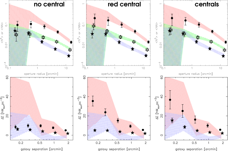
Figure 13: Average fit, compared to the observation, of the ${\cal N}$-statistics (first row; points: variance of red galaxies, filled stars: variance of blue galaxies, open stars: cross-correlation) and GGL (second row; filled stars: blue galaxies, points: red galaxies) as predicted by the three different halo-model scenarios (first column: no central galaxies, second column: red central galaxies, third column: blue and red central galaxies) for the redshift bin $\bar{z}=0.7$. The model fits (average over the MCMC tracks) and their $1\sigma$-variance are denoted by points and errorbars, the shaded areas bracket the $1\sigma$-range in COMBO-17. For the GGL panels shaded areas are the combined constraints from all redshift bins. The corresponding model predictions for the number density of red galaxies are (in units of $h^{3}\rm Mpc^{-3}$) $11\pm 8\times 10^{-3}$ (no central), $8\pm 4\times 10^{-3}$ (red central), $9\pm 6\times 10^{-3}$ (red and blue centrals) and for blue galaxies $51\pm 15\times 10^{-3}$ (no central), $57\pm 18\times 10^{-3}$ (red central), $65\pm 21\times 10^{-3}$ (red and blue centrals).

6.3.2 Results

Fig. 13 shows the model fits to the data belonging to the redshift bin $\bar{z}=0.7$. This redshift bin was chosen since it has the best signal-to-noise in our data.

Table 4: Quality of the halo model fits and a Bayesian comparison of the three different models describing the same data. The $\chi^{2}/{\rm dof}$ per degree of freedom (${\rm dof}=26-13=13$) is for the maximum-likelihood fit to the data. By $\Delta\ln{E}$ we mean the difference of the Bayesian (log)evidence for a particular scenario relative to the scenario with the highest evidence at the same redshift.

$\bar{z}$	$\chi^{2}/{\rm dof}$	$\Delta\ln{E}$	model type
0.3	0.51	0.00	no central galaxies
0.3	0.56	0.44	red central galaxies
0.3	0.45	0.57	blue and red centrals
0.5	1.25	0.00	no central galaxies
0.5	1.20	0.86	red central galaxies
0.5	1.24	0.88	blue and red centrals
0.7	0.57	0.00	no central galaxies
0.7	0.50	1.02	red central galaxies
0.7	0.60	1.19	blue and red centrals
0.9	0.59	0.00	red central galaxies
0.9	0.55	0.07	blue and red centrals
0.9	0.62	0.31	no central galaxies

Note that the points (model prediction) in this figure are the model averages along the MCMC tracks and not the best-fitting models (minimum $\chi^{2}$). The $1\sigma$-standard deviation of the fits is denoted by error bars. The MCMC-average is useful to study how well a model fits the data in general and where the main problems of the model in describing the data are located.

We gather from this figure that, in general, qualitatively all three model scenarios appear to provide a pretty good description of the data. The main differences appear for $\theta_{\rm ap}\lesssim 1^{\prime}$ (${\cal N}$-statistics) and $\theta\lesssim 0^{\prime}\!\!.5$ (GGL); the differences in the $\cal N$-statistics are small, though. The scenario with no central galaxies at all is bound to systematically smaller values for the ${\cal N}$-statistics and, thus, has small difficulties in explaining the clustering statistics of red galaxies for smaller scales. Since statistical uncertainties grow large for small scales, those difficulties are not too significant for our data.

Three other issues can be identified:

• Although the galaxy clustering and the GGL is well described by the models, there is only moderate agreement between the predicted and observed mean number densities of blue galaxies: the predicted numbers are higher. The measured value (Table 1) is, however, still within the $2\sigma$-scatter of $\bar{n}_{\rm blue}$ of the Markov chains. For example, for $\bar{z}=0.7$ the model predicts consistently for all scenarios $\bar{n}_{\rm blue}\sim(57\pm 18)\times 10^{-3}\,h^{3}\rm Mpc^{-3}$, whereas the data estimate is $\bar{n}_{\rm blue}=(18\pm 3)\times 10^{-3}\,h^{3}\rm Mpc^{-3}$. This could point towards an inaccuracy of the halo model or/and to a systematic underestimate of $\bar{n}_{\rm blue}$ provided by the $V_{\rm max}$-estimator. The observed numbers of red galaxies are always within the $1\sigma$-scatter of the Markov chains although the means of the chains are always larger than the observed values, which again could be indicative of an overprediction by our halo-model. Tensions between the halo model predictions for galaxy clustering and number densities were also noticed by other studies, such as Quadri et al. (2008).

• The GGL-signal of the blue galaxies always conflicts the data beyond $\theta\gtrsim 0^{\prime}\!.5$ (too high) because the observed $\Delta\Sigma$ quickly drops to essentially negative in that regime (if the GGL of all redshift bins is combined). Considering that most of the other model predictions fit quite well and that, to the knowledge of the authors, no negative GGL-signal for these galaxy separations has been found in the literature, this conflict could very well be a hint towards systematics in the lensing data undiscovered so far.

• The model without red central galaxies is in mild conflict with the GGL measurement for the smallest separations: a galaxy centred on the halo centre boosts the GGL signal, which is arguably favoured by the data (when the GGL-signal of all redshift bins is combined).

Table 4 lists the (reduced) $\chi^{2}$ of the maximum likelihood fits and the estimated Bayesian evidence of the three different model scenarios. All scenarios at all redshifts give good fits to the data. The worst fits, $\chi^{2}/{\rm dof}\sim 1.25$, are for the redshift bin $\bar{z}=0.5$ which may be related to the sudden drop of the ${\cal N}$-statistics for the largest aperture radius (upper right panel in Fig. 6). Since this $\chi^{2}$ still has a probability of $\sim 20\%$, we can consider it as a statistical fluke.

Except for $\bar{z}=0.7$, where we find weak evidence for a model without central galaxies, the Bayesian model discrimination does not prefer any particular model. Combining the evidence of all redshift bins (the Bayesian evidence just sums up), assuming independent statistical information, however yields substantial evidence ($\Delta\ln{E}\approx 2$) for a model without central galaxies. On the other hand, by looking at Fig. 13 we concluded that a model without central galaxies has some problems describing the data on the smallest scales. Moreover, our central galaxy models have always, except for $\bar{z}=0.3$, a better $\chi^{2}$. All of which taken together makes us suspicious, if the Laplacian approximation that is used to compute the Bayesian evidence is really accurate enough for our work. Our model comparison therefore seems to be inconclusive and an improved statistical analysis or a larger data set will have to revisit this question in the future.

Table 5 (after the bibliography) lists the constraints on the halo-model parameters for all redshifts and all scenarios. For an parameter average over all redshifts (bottom block of table), we combine the 1D-probability density functions (PDFs), $P_{i}(p_{j})$, as estimated from the MCMCs, of all parameters, $p_{j}$, for all redshifts $i$ to obtain a total 1D-posterior of $p_{j}$:

$$P(p_{j})=\prod_{i}P_{i}(p_{j})\;.$$ (75)

From this total posterior we derive the mean and r.m.s.-variance of every parameter. Note that for top-hat and equal $P_{i}$’s one has $P=P_{i}$, meaning combining information does not improve anything in this case.

First of all, we find that the fits seem to be robust with respect to the three different model scenarios, with $R$, $f$ and maybe $m^{\prime}$ being the only possible exceptions.

For all aforementioned parameters, we do not see a clear trend with redshift, maybe with $m_{\rm min}$ being an exception which (the median) is increasing slightly in $\bar{z}=0.9$ but still is consistent with the rest. The redshift-combined result of this parameter is $m_{\rm min}=10^{12.1\pm 0.2}h^{-1}{\rm M}_{\odot}$ for red and $m_{\rm min}=10^{11.2\pm 0.1}h^{-1}{\rm M}_{\odot}$ for blue galaxies. Therefore, blue-cloud galaxies clearly populate smaller haloes than red-sequence galaxies. In fact, this is the halo-model explanation for the different clustering strengths of red and blue galaxies.

The combined result for the parameter pair $m^{\prime}$ and $\epsilon$, describing the galaxy occupancy as function of halo mass beyond $m_{\rm min}$, is roughly for both red and blue galaxies $m^{\prime}=10^{13.0\pm 0.4}h^{-1}{\rm M}_{\odot}$ and $\epsilon=1.1\pm 0.2,1.3\pm 0.2$ for red and blue galaxies, respectively.

The least constrained parameter in our analysis is clearly $\sigma_{\log{m}}$ which has for all redshifts $0.5\pm 0.2$. This is essentially what one would expect from a top-hat PDF, non-vanishing between $0\ldots 1$. Therefore, our data does not add information that significantly improves our prior. Combining all redshifts shrinks the $1\sigma$-confidences somewhat, though, because the individual 1D-PDFs are not completely flat.

Apparently only little more information is added to $\lambda$, the HOD variance parameter, by the data. With a top-hat prior between $0.9\ldots 10$ we would expect as constraint $\lambda=5.5\pm 2.5$, which is roughly what we find for the individual redshift bins, excluding $\lambda$ of blue galaxies for the model with red central galaxies only. However, the 1D-PDFs are not completely flat preferring some regions in parameter space, too. In particular, they exclude values near $\lambda\sim 1$ which is the HOD variance in the “Poisson satellite” model. As discussed earlier, this is because $\lambda=1$ cannot explain the observed deep drop in $r(\theta_{\rm ap})$ for small scales. Quantitatively, we infer from the redshift-combined PDF of $\lambda$ that we can decisively exclude values less than $\lambda=2$ for red galaxies and $\lambda=3$ for blue galaxies with $95\%$ confidence. This fits to the findings of Collister & Lahav (2005) that found no indications of a sub-Poissonian variance, $\alpha(m)<1$, in their analysis of red and blue galaxies.

For the combined concentration parameter of red and blue galaxies we find values that depend slightly on the adopted scenario. In a model with no central galaxies, red galaxies require a concentration larger than that of dark matter, $f_{\rm red}=1.9\pm 0.5$, which, however drops to $f_{\rm red}\approx 1.3\pm 0.5$ if a central red galaxy is allowed. Our conclusion is that the data demands a centrally concentrated spatial distribution of red galaxies either by a larger $f_{\rm red}$ or by a central galaxy. Conversely, for blue galaxies we find for no central galaxies, $f_{\rm blue}=1.0\pm 0.4$, consistent with the dark matter distribution, but distributions flatter than dark matter, $f_{\rm blue}=0.6\pm 0.3$, if central galaxies are present.

The JHOD correlation factor, $R$, turns out to be hard to measure. For the individual redshift bins we find little improvement compared to the flat prior. For all $z$-bins combined, we find $R=+0.1\pm 0.2$ (no central galaxies/only red central galaxies) and $R=+0.5\pm 0.2$ (blue and red central galaxies). This implies that the number of red and blue galaxies are uncorrelated in the first case and slightly positively correlated in the latter case.

Inside Fig. 7 we plotted the bestfit solutions to the relative linear stochastic bias of the red and blue population found along the MCMC tracks for a mean redshift of $\bar{z}=0.7$. The halo model reproduces the scale-dependence of bias factor and correlation factor at that redshift well (note that the shaded confidence regions are combinations of all redshift bins). All three scenarios reveal very similar trends with most differences for very small scales which, however due to measurement noise (galaxy shot noise), are not well constrained. If we use the halo model and bestfit parameters to extrapolate the bias parameters to large scales we find a bias factor between $b\sim 1.46-1.58$ depending on the particular scenario. Those values reconcile our measurements at relatively small scales with results from various other studies that measured galaxy biasing on larger scales (see Sect. 4.3). Furthermore, it underlines the need for both small and large scale measurements of galaxy clustering in order to discriminate different halo-model scenarios. In that context, we also would like to point to Fig. 13, lower row. Here we can easily see that the three halo-model scenarios predict clearly different GGL for galaxy separations smaller than $\sim 12^{\prime\prime}\!$, corresponding to a physical scale of $\sim 60\,h^{-1}\rm kpc$. This shows that GGL has an important model discriminating power on those scales. However, the halo model outlined here may be inaccurate on exactly those scales as it does not include the effect of lenses hosting individual haloes inside their parent halo (Sheth & Jain, 2003). Unfortunately, the statistical uncertainties in our GGL measurements do not allow to fully exploit this potential.

7 Summary

For this paper we studied the clustering and, in particular, the relative clustering of red sequence galaxies and blue-cloud galaxies in COMBO-17  (fields: S11, A901, CDFS) inside four redshift bins up to a redshift of $z\sim 1$. The two samples were separated by applying a redshift-dependent cut along the red-sequence. An additional cut was applied to assure that red and blue galaxies at all redshifts have roughly the same colour-dependent $M_{V}$-limits. The red sample has $\langle M_{V}\rangle=-20.0\pm 0.1\,\rm mag$, the blue sample has $\langle M_{V}\rangle=-18.8\pm 0.1\,\rm mag$ ($h=1.0$).

By looking at the spatial correlation function of the samples, we found for all redshifts combined a correlation length of $r_{0}=5.5\pm 0.9,3.0\pm 0.4\,h^{-1}\rm Mpc$ for the red and blue galaxies, respectively. The corresponding power-law indices of the spatial correlation function were $\delta=0.85\pm 0.10,0.65\pm 0.08$. A significant evolution of these parameters with redshift was not found.

Parameterising the relative biasing of the red and blue sample in terms of the linear stochastic bias, we measured for all redshifts combined that the bias factor, $b(\theta_{\rm ap})$, is slightly scale-dependent within a range of aperture radii of $\theta_{\rm ap}=6^{\prime\prime}\!-20^{\prime}$, varying between $b\sim 1.7-2.2$. We found that the second parameter, $r(\theta_{\rm ap})$ – quantifying the correlation of galaxy number density fluctuations as function of scale –, is scale-dependent, too. It drops from a value close to unity at larger scales of $\theta_{\rm ap}\sim 20^{\prime}$ to $r\sim 0.6\pm 0.15$ at $\theta_{\rm ap}\sim 6^{\prime\prime}\!$. An aperture radius of $\theta_{\rm ap}=10^{\prime}$ corresponds to a proper spatial scale of $2.8,3.8,4.5,4.8\,h^{-1}\rm Mpc$ at the redshifts $z=0.3,0.5,0.7,0.9$, respectively. The measurements emphasise the different clustering of the red and blue sample at all redshifts, but do not exhibit a clear evolution with redshift beyond the statistical uncertainties.

We also looked at the mean tangential ellipticity of a population of faint background galaxies as function of separation from red and blue galaxies (GGL). For this analysis, shear catalogues with a mean source redshift of $\bar{z}=0.78$ from the GaBoDS were taken. The GGL-signal detected corresponds to a projected differential surface mass density of $\Delta\Sigma=35\pm 25\,h\rm{\rm M}_{\odot}pc^{-2}$, red galaxies, and $\Delta\Sigma=16\pm 10\,h\rm{\rm M}_{\odot}pc^{-2}$, blue galaxies, at a galaxy-galaxy separation of $\sim 12^{\prime\prime}\!$ (roughly $\sim 60\,h^{-1}\rm kpc$). This indicates that the red galaxies are either typically more massive than blue galaxies, or are residing inside a matter richer environment than the blue galaxies.

A large part of the paper discussed a dark-matter halo based model that was employed to describe the angular clustering, including the cross-correlation function of clustering, the GGL-signal and the (ratio of) number densities of the red and blue galaxy sample simultaneously. Due to large statistical errors for the GGL, the GGL-signal mainly served as an upper limit for a model predicted signal.

We used three different variants of our halo-model, all having the same number of free parameters, to fit the data: i) neither the red nor the blue population have central galaxies, ii) only the red sample has central galaxies, and iii) both the red and blue sample can have central galaxies and there is always one central galaxy. A Bayesian method of model discrimination was performed to decide which model at which redshift may be most suitable in explaining the data. The model discrimination was inconclusive, a more accurate treatment or a larger data set is required. In this context, we pointed out that GGL at small separations is most sensitive to the presence or absence of a central galaxy.

Describing the cross-correlation function required the extension of the halo-model descriptions currently available in the literature by at least one additional parameter (see Scranton (2003, 2002) which is equivalent to our approach only if $R(m)=0$). The extension is necessary for a full parametrisation of the $2^{\rm nd}$-order joint HOD of two galaxy populations. We called this parameter the correlation factor of the joint HOD of two galaxy populations, $R(m)$. It expresses the tendency of different galaxy types to avoid ($R(m)$ close to minus unity) or attract each other ($R(m)$ close to plus unity) inside/into a same dark matter halo of mass $m$. A vanishing $R(m)$ indicates uncorrelated halo-occupation numbers. The $2^{\rm nd}$-order cross-correlation function of two galaxy samples, or equivalently $r(\theta_{\rm ap})$, is most sensitive to $R(m)$ for small separations where the one-halo term is dominating ($\theta_{\rm ap}\lesssim 20^{\prime}$ for $\bar{z}=0.3$). In principle, $R(m)$ is halo-mass dependent but its impact on the cross-correlation function becomes negligible for haloes with large galaxy occupation numbers (large $m$). Therefore, observations mainly constrain $R(m)$ for smaller haloes. The measurements of $R$ for the individual $z$-bins yielded only little constraints. Combining all redshifts we found $R=+0.5\pm 0.2$ (positive correlation of galaxy numbers) for iii) and $R=+0.1\pm 0.2$ for i) and ii) (no correlation).

We found it necessary to add another new degree of freedom, $\lambda$, to the model in order to explain the observed, towards smaller scales declining sub-unity bias parameter $r(\theta_{\rm ap})$. The parameter $\lambda$ regulates how quickly a HOD of galaxy numbers populating a dark-matter halo assumes a Poisson variance, see Sect. 6.2.2 for an explanation. We demonstrated that the cross-correlation function of galaxy clustering is quite sensitive to $\lambda$: $r(\theta_{\rm ap})$ seems to reach values substantially smaller than unity only for $\lambda>1$. With all models i)-iii) we decisively excluded, for red and blue galaxies, a value of $\lambda\lesssim 2$ (red) and $\lambda\lesssim 3$ (blue) with $95\%$ confidence. This rules out with high confidence, at least for our red and blue galaxy samples, a model like that of Kravtsov et al. (2004) (“Poisson satellites”) for the mean number of galaxy pairs inside a halo.

The halo model parameters of the red and blue sample mostly differ for $m_{\rm min}$. We concluded that the average of the mass-scale for $z=0\ldots 1$ is $m_{\rm min}=10^{12.1\pm 0.2}h^{-1}{\rm M}_{\odot}$ for red and $m_{\rm min}=10^{11.2\pm 0.1}h^{-1}{\rm M}_{\odot}$ for blue galaxies.

Finally, we presented evidence that red galaxies are more concentrated towards the halo centre than the dark matter, which either has to be achieved by a central red galaxy or a larger concentration parameter $f_{\rm red}=1.9\pm 0.5$. The distribution of blue galaxies is consistent with the dark matter distribution inside a halo for i), but flatter with $f_{\rm blue}=0.6\pm 0.3$ for ii) or iii).

As an outlook, we would like to mention that the joint HOD of two galaxy populations is also probed by a new statistics, third-order galaxy-galaxy lensing (red and blue galaxies as lenses), that are outlined in Schneider & Watts (2005) and have been recently detected for the first time in Simon et al. (2008). Combining those statistics with the second-order cross-correlation function in forthcoming surveys promises to set better constraints on the JHOD correlation factor.

Table 5: Compilation of MCMC results for the halo model parameters (see Section 6.2), obtained from fitting three different model scenarios to the ${\cal N}$-statistics, relative galaxy numbers and GGL-signal. The three scenarios are denoted by “S” (simple, no central galaxies), “M” (mixed, only red central galaxies) and “C” (central, red and blue central galaxies), respectively. The parameters of $m_{\rm min}$ and $m^{\prime}$ are in units of solar masses, $h^{-1}{\rm M}_{\odot}$, the parameter $R$ represents the JHOD correlation factor between the red and blue sample. Quoted parameter values stand for median and $1\sigma$ confidence limits as derived from the MCMCs. The last block of values at the bottom of the table contains constraints (mean and r.m.s. variance) from all redshifts combined. The fiducial cosmological model uses WMAP3 parameters.

	RED SAMPLE						BLUE SAMPLE
$\bar{z}$	$[\log_{10}{m_{\rm min}}$	$\sigma_{{\rm log}m}$	$\log_{10}{m^{\prime}}$	$\epsilon$	$f$	$\lambda$]	$[\log_{10}{m_{\rm min}}$	$\sigma_{{\rm log}m}$	$\log_{10}{m^{\prime}}$	$\epsilon$	$f$	$\lambda$]	$R$	type
$0.3$	$12.1^{+0.5}_{-0.4}$	$0.5^{+0.3}_{-0.3}$	$13.9^{+1.5}_{-1.5}$	$1.0^{+0.5}_{-0.4}$	$1.7^{+0.9}_{-0.9}$	$4.3^{+2.9}_{-2.0}$	$11.0^{+0.3}_{-0.3}$	$0.5^{+0.3}_{-0.3}$	$13.6^{+1.6}_{-0.9}$	$1.1^{+0.5}_{-0.5}$	$1.5^{+1.0}_{-0.9}$	$4.5^{+2.6}_{-2.0}$	$+0.0^{+0.6}_{-0.6}$	S
$0.3$	$11.9^{+0.3}_{-0.2}$	$0.5^{+0.3}_{-0.3}$	$12.6^{+1.6}_{-1.4}$	$0.8^{+0.5}_{-0.4}$	$1.3^{+1.0}_{-0.8}$	$5.0^{+3.1}_{-2.7}$	$10.9^{+0.2}_{-0.2}$	$0.5^{+0.3}_{-0.3}$	$13.0^{+1.7}_{-0.6}$	$1.1^{+0.4}_{-0.5}$	$0.6^{+0.8}_{-0.4}$	$5.5^{+2.8}_{-2.5}$	$+0.0^{+0.5}_{-0.5}$	M
$*0.3$	$11.8^{+0.3}_{-0.3}$	$0.5^{+0.3}_{-0.3}$	$12.9^{+0.9}_{-0.8}$	$1.0^{+0.4}_{-0.3}$	$1.4^{+0.9}_{-0.9}$	$5.3^{+3.0}_{-2.8}$	$10.8^{+0.3}_{-0.2}$	$0.5^{+0.3}_{-0.3}$	$12.8^{+0.7}_{-0.5}$	$1.2^{+0.4}_{-0.3}$	$1.2^{+1.0}_{-0.8}$	$3.9^{+3.0}_{-2.0}$	$+0.3^{+0.5}_{-0.6}$	C
$0.5$	$12.2^{+0.2}_{-0.2}$	$0.5^{+0.3}_{-0.3}$	$13.9^{+1.3}_{-1.7}$	$0.7^{+0.6}_{-0.4}$	$1.9^{+0.7}_{-0.9}$	$5.5^{+2.6}_{-2.6}$	$11.3^{+0.2}_{-0.2}$	$0.5^{+0.3}_{-0.3}$	$13.1^{+1.8}_{-0.8}$	$1.0^{+0.4}_{-0.4}$	$0.9^{+0.8}_{-0.5}$	$4.9^{+3.0}_{-2.4}$	$+0.2^{+0.5}_{-0.5}$	S
$0.5$	$12.0^{+0.2}_{-0.2}$	$0.5^{+0.3}_{-0.3}$	$12.3^{+1.5}_{-1.0}$	$0.6^{+0.3}_{-0.3}$	$1.3^{+0.9}_{-0.7}$	$5.2^{+2.9}_{-2.7}$	$11.2^{+0.2}_{-0.1}$	$0.5^{+0.3}_{-0.3}$	$12.7^{+1.0}_{-0.6}$	$0.9^{+0.4}_{-0.4}$	$0.5^{+0.4}_{-0.2}$	$6.0^{+2.4}_{-2.6}$	$+0.2^{+0.5}_{-0.5}$	M
$0.5$	$12.0^{+0.2}_{-0.2}$	$0.5^{+0.3}_{-0.3}$	$12.6^{+1.0}_{-0.8}$	$0.7^{+0.3}_{-0.3}$	$1.4^{+0.9}_{-0.8}$	$5.2^{+2.9}_{-2.7}$	$11.2^{+0.2}_{-0.2}$	$0.5^{+0.3}_{-0.3}$	$12.6^{+0.7}_{-0.5}$	$1.0^{+0.3}_{-0.3}$	$0.4^{+0.5}_{-0.2}$	$4.7^{+3.2}_{-2.2}$	$+0.6^{+0.3}_{-0.5}$	C
$0.7$	$12.0^{+0.3}_{-0.2}$	$0.5^{+0.3}_{-0.3}$	$13.2^{+0.3}_{-0.3}$	$1.6^{+0.3}_{-0.3}$	$1.8^{+0.8}_{-0.8}$	$5.3^{+2.8}_{-2.7}$	$11.1^{+0.1}_{-0.1}$	$0.5^{+0.3}_{-0.3}$	$13.0^{+0.2}_{-0.3}$	$1.7^{+0.2}_{-0.3}$	$1.2^{+0.8}_{-0.5}$	$6.9^{+1.9}_{-2.1}$	$+0.1^{+0.5}_{-0.5}$	S
$0.7$	$12.0^{+0.2}_{-0.2}$	$0.5^{+0.3}_{-0.3}$	$13.1^{+0.3}_{-0.4}$	$1.5^{+0.3}_{-0.3}$	$1.6^{+0.8}_{-0.8}$	$5.3^{+2.7}_{-2.8}$	$11.1^{+0.1}_{-0.1}$	$0.5^{+0.3}_{-0.3}$	$12.9^{+0.2}_{-0.2}$	$1.6^{+0.2}_{-0.2}$	$0.8^{+0.6}_{-0.4}$	$7.7^{+1.5}_{-1.9}$	$-0.2^{+0.5}_{-0.4}$	M
$0.7$	$12.1^{+0.2}_{-0.2}$	$0.5^{+0.3}_{-0.3}$	$13.1^{+0.3}_{-0.4}$	$1.5^{+0.3}_{-0.2}$	$1.5^{+0.9}_{-0.8}$	$5.1^{+3.1}_{-3.1}$	$11.1^{+0.1}_{-0.1}$	$0.5^{+0.3}_{-0.3}$	$12.7^{+0.3}_{-0.3}$	$1.4^{+0.2}_{-0.2}$	$0.9^{+0.7}_{-0.5}$	$6.5^{+2.2}_{-2.3}$	$+0.3^{+0.5}_{-0.6}$	C
$0.9$	$12.5^{+0.3}_{-0.3}$	$0.5^{+0.3}_{-0.3}$	$14.5^{+1.0}_{-1.8}$	$0.9^{+0.6}_{-0.5}$	$1.7^{+0.8}_{-0.9}$	$4.5^{+3.0}_{-2.2}$	$11.5^{+0.2}_{-0.2}$	$0.5^{+0.3}_{-0.3}$	$14.5^{+1.0}_{-1.2}$	$1.2^{+0.5}_{-0.5}$	$1.2^{+1.0}_{-0.7}$	$4.5^{+2.3}_{-1.9}$	$-0.1^{+0.6}_{-0.5}$	S
$0.9$	$12.5^{+0.3}_{-0.3}$	$0.5^{+0.3}_{-0.3}$	$14.4^{+1.1}_{-2.1}$	$0.9^{+0.6}_{-0.5}$	$1.5^{+0.9}_{-0.9}$	$4.4^{+3.3}_{-2.3}$	$11.4^{+0.2}_{-0.2}$	$0.5^{+0.3}_{-0.3}$	$14.4^{+1.0}_{-1.2}$	$1.1^{+0.5}_{-0.6}$	$0.6^{+0.7}_{-0.4}$	$5.7^{+2.3}_{-2.2}$	$+0.1^{+0.6}_{-0.6}$	M
$0.9$	$12.5^{+0.3}_{-0.3}$	$0.4^{+0.3}_{-0.3}$	$14.2^{+1.2}_{-1.6}$	$0.8^{+0.6}_{-0.5}$	$1.1^{+1.2}_{-0.9}$	$4.7^{+2.9}_{-2.4}$	$11.7^{+0.2}_{-0.3}$	$0.5^{+0.3}_{-0.3}$	$14.5^{+1.1}_{-1.4}$	$1.2^{+0.5}_{-0.5}$	$1.0^{+1.1}_{-0.7}$	$3.9^{+2.1}_{-1.7}$	$+0.5^{+0.3}_{-0.6}$	C
ALL	$12.2^{+0.2}_{-0.2}$	$0.5^{+0.2}_{-0.2}$	$13.4^{+0.7}_{-0.7}$	$1.3^{+0.3}_{-0.3}$	$1.9^{+0.5}_{-0.5}$	$4.3^{+1.6}_{-1.6}$	$11.2^{+0.1}_{-0.1}$	$0.5^{+0.2}_{-0.2}$	$13.0^{+0.2}_{-0.2}$	$1.4^{+0.2}_{-0.2}$	$1.0^{+0.4}_{-0.4}$	$5.3^{+1.4}_{-1.4}$	$+0.1^{+0.2}_{-0.2}$	S
ALL	$12.1^{+0.1}_{-0.1}$	$0.5^{+0.2}_{-0.2}$	$12.9^{+0.4}_{-0.4}$	$1.1^{+0.2}_{-0.2}$	$1.3^{+0.5}_{-0.5}$	$4.4^{+1.9}_{-1.9}$	$11.2^{+0.1}_{-0.1}$	$0.5^{+0.2}_{-0.2}$	$12.9^{+0.2}_{-0.2}$	$1.4^{+0.2}_{-0.2}$	$0.5^{+0.2}_{-0.2}$	$7.0^{+1.3}_{-1.3}$	$+0.1^{+0.2}_{-0.2}$	M
ALL	$12.1^{+0.1}_{-0.1}$	$0.5^{+0.2}_{-0.2}$	$13.1^{+0.3}_{-0.3}$	$1.1^{+0.2}_{-0.2}$	$1.4^{+0.5}_{-0.5}$	$5.1^{+1.4}_{-1.4}$	$11.1^{+0.1}_{-0.1}$	$0.5^{+0.2}_{-0.2}$	$12.8^{+0.2}_{-0.2}$	$1.3^{+0.2}_{-0.2}$	$0.6^{+0.3}_{-0.3}$	$4.8^{+1.2}_{-1.2}$	$+0.5^{+0.2}_{-0.2}$	C

Appendix A Dark matter halo properties of model

For $n(m)$, we use the semi-analytical peak-background split prescription of Sheth & Tormen (1999):

$$n(m)\propto\frac{1}{m^{2}}\frac{\sqrt{a}\nu}{1+[a\nu^{2}]^{-p}}{\rm e}^{-\frac{a\nu^{2}}{2}}\frac{{\rm d}\ln{\nu^{2}}}{{\rm d}\ln{m}}$$ (76)

with $\nu=\delta_{\rm c}/(D(z)\sigma(m))$, $a=0.707$ and $p=0.3$. The expression

$$\sigma(m)=\frac{9}{2\pi^{2}}\int_{0}^{\infty}{\rm d}kk^{2}\,\frac{[\sin{(rk)}-rk\cos{(rk)}]^{2}}{(rk)^{6}}P_{\rm lin}(k)$$ (77)

denotes the top-hat variance of the linear dark matter fluctuations, within spheres of radius $r=\left(\frac{3m}{4\pi\rho_{\rm crit}\Omega_{\rm m}}\right)^{1/3}$. The function $D(z)$ denotes the linear growth factor, to be normalised to one for $z=0$ (Peebles, 1980):

$$D(z)\propto H(a(z))\int_{0}^{(1+z)^{-1}}{\rm d}a\frac{1}{[aH(a)]^{3}}\;,$$ (78)

where $a(z)=(1+z)^{-1}$ is the cosmological scale factor and $H(a)$ the Hubble parameter. The constant $\delta_{\rm c}$, the over-density of virialised haloes undergoing linear spherical collapse at $z=0$, is chosen according to Nakamura & Suto (1997):

$$\delta_{\rm c}=\frac{3(12\pi)^{2/3}}{20}\left[1+0.0123\log_{10}{\Omega_{\rm m}}\right]\;.$$ (79)

For the cosmology adopted in this paper, one finds $\delta_{\rm c}=1.674$. For the linear dark matter power spectrum the prescription of Eisenstein & Hu (1998) is employed. It is evolved to redshift $z$ using the linear growth factor $D(z)$.

The halo bias function we implemented into our model is from Tinker et al. (2005) which is a modification of the original function of Sheth et al. (2001):

$$b(m)=1+\frac{1}{\sqrt{a}\delta_{\rm c}}\times$$ (80)

$$\left[\sqrt{a}(a\nu^{2})+\sqrt{a}b(a\nu^{2})^{1-c}-\frac{(a\nu^{2})^{c}}{(a\nu^{2})^{c}+b(1-c)(1-c/2)}\right]$$

with $a=0.707$, $b=0.35$, $c=0.8$ and $\nu$ as previously defined. To guarantee that, when using this prescription for $b(m)$, the two-halo term asymptotically fits the linear dark matter power spectrum $P_{\rm lin}(k)$ on large-scales (small $k$) we artificially normalise all $P^{\rm 2h}_{ij}(k)$ in Eq. (6.1.1) by (see e.g. Mandelbaum et al., 2005)

$$\bar{b}^{2}\equiv\left[\frac{1}{\overline{m}}\int{\rm d}m\,n(m)\,b(m)\right]^{2}\;.$$ (81)

This normalisation is $\bar{b}=1.02,1.08$ for $z=0.0,1.0$.

The dark matter density profile of haloes is in our model a truncated NFW (Navarro et al., 1996):

$$u_{0}(r,m)\propto\left\{\begin{array}[]{ll}\frac{1}{\frac{r}{r_{\rm s}}\left(1+\frac{r}{r_{\rm s}}\right)^{2}}&{\rm for~{}}r\leq r_{\rm vir}\\ 0&{\rm otherwise}\end{array}\right.\;,$$ (82)

with $r_{\rm s}\equiv\frac{r_{\rm vir}}{c(m,z)}$ with $r_{\rm vir}^{3}=\frac{3m}{4\pi\rho_{\rm crit}\Omega_{\rm m}\Delta_{\rm vir}(z)}$ and $c(m,z)$ being the so-called viral radius and concentration parameter, respectively. For the over-density within the virial radius we use (Bullock et al., 2001):

$$\Delta_{\rm vir}(z)=\frac{18\pi^{2}+82(\Omega_{\rm m}(z)-1)-39(\Omega_{\rm m}(z)-1)^{2}}{\Omega_{\rm m}(z)}\;,$$ (83)

$\rho_{\rm crit}$ (at redshift $z=0$) and $\Omega_{\rm m}(z)$ are the critical matter density and matter density parameter, respectively; $\Omega_{\rm m}\equiv\Omega_{\rm m}(z=0)$. The concentration parameter is calculated according to Seljak (2000):

$$c(m,z)=\frac{10}{1+z}\left(\frac{m}{m_{\ast}}\right)^{-0.20}\;,$$ (84)

where the present day non-linear mass scale, $m_{\ast}$, is defined by $\delta_{\rm c}=\sigma(m_{\ast})$. For our adopted cosmology we find $m_{\ast}=1.9\times 10^{12}h^{-1}{\rm M}_{\odot}$.

Appendix B Exact statistical moments for central galaxy models

As can be seen in Table 3, in a scenario where we split the halo occupation number of one population (mixed scenario) or both populations (pure central scenario) into one central galaxy and satellite galaxies one has to specify $\langle N_{i}^{\rm sat}N_{j}^{\rm cen}\rangle$, $\langle N_{i}^{\rm sat}N_{j}^{\rm sat}\rangle$ or $\langle N_{i}^{\rm sat}N_{j}\rangle$, $\langle N_{i}^{\rm cen}N_{j}\rangle$ as function of halo mass $m$, respectively. Here, we give general expressions in terms of the JHOD, $P(N_{i},N_{j}|m)$, of these moments. A detailed derivation for one of the moments is given, the others can be obtained in a similar manner. Note that we skip the arguments “$(m)$” and “$|m$” in the JHOD for the derivation; all following equations are for haloes of a fixed mass.

The central galaxy-satellite splitting is done in such a way that we always have $N^{\rm cen}=1$ if $N\geq 1$, $N^{\rm cen}=0$ for $N=0$, $N^{\rm sat}=N-1$ for $N>1$ and $N^{\rm sat}=0$ for $N\leq 1$. This is to say that (${\rm H}(x)$ is the Heaviside step function):

$$N_{i}^{\rm sat} = {\rm H}\left(N_{i}-1\right)\left(N_{i}-1\right)\;,$$ (85)

$$N_{i}^{\rm cen} = {\rm H}\left(N_{i}-1\right)\;.$$ (86)

We focus on $\langle N_{i}^{\rm sat}N_{j}^{\rm cen}\rangle$. Let us substitute the previous expressions and write down explicitly the ensemble average in the statistical moment as sum over the JHOD (the states, halo occupation numbers, are integers), taking into account the Heaviside step functions:

$$\!\!\!\!\!\!\!\!\!\big{\langle}N_{i}^{\rm sat}N_{j}^{\rm cen}\big{\rangle}=\sum_{N_{i}=1}^{\infty}\sum_{N_{j}=1}^{\infty}\left(N_{i}-1\right)P(N_{i},N_{j})$$ (87)

$$= \sum_{N_{i}=0}^{\infty}\sum_{N_{j}=0}^{\infty}\left(N_{i}-1\right)P(N_{i},N_{j})$$

$$- \sum_{N_{i}=0}^{\infty}\sum_{N_{j}=0}^{0}\left(N_{i}-1\right)P(N_{i},N_{j})$$

$$- \sum_{N_{i}=0}^{0}\sum_{N_{j}=0}^{\infty}\left(N_{i}-1\right)P(N_{i},N_{j})$$

$$+ \sum_{N_{i}=0}^{0}\sum_{N_{j}=0}^{0}\left(N_{i}-1\right)P(N_{i},N_{j})$$

$$= \big{\langle}N_{i}\big{\rangle}-1-\sum_{N_{i}=0}^{\infty}\left(N_{i}-1\right)P(N_{i}|N_{j}=0)$$

$$+ \sum_{N_{j}=0}^{\infty}P(N_{j}|N_{i}=0)-\sum_{N_{i},N_{j}=0}^{0}P(N_{i},N_{j})$$

$$= \big{\langle}N_{i}\big{\rangle}-1-\big{\langle}N_{i}|N_{j}=0\big{\rangle}+P(N_{j}=0)$$

$$+ P(N_{i}=0)-P(N_{i}=0,N_{j}=0)$$

$$= \big{\langle}N_{i}\big{\rangle}-1-\big{\langle}N_{i}|N_{j}=0\big{\rangle}+P(N_{i}N_{j}=0)\;,$$

where we denote by

$$\big{\langle}N_{i}|N_{j}=0\big{\rangle}\equiv\sum_{N_{i}=0}^{\infty}N_{i}P(N_{i},N_{j}=0)$$ (88)

the conditional halo-average of $N_{i}$ for which $N_{j}=0$, whereas $P(N_{i}N_{j}=0)$ denotes the probability to find a halo which has either $N_{i}=0$ or $N_{j}=0$. The conditional mean is zero, if all haloes have at least one $j$-galaxy. We have used in the foregoing calculus the relations (also with $i$ and $j$ interchanged)

$$P(N_{i}) \!\!=\!\! \sum_{N_{j}=0}^{\infty}\,P(N_{i},N_{j})\;,$$ (89)

$$P(N_{i}N_{j}\!=\!0) \!\!=\!\! P(N_{i}\!=\!0)+P(N_{j}\!=\!0)-P(N_{i}\!=\!0,N_{j}\!=\!0)$$

and

$$\sum_{N_{i}=0}^{0}\sum_{N_{j}=0}^{\infty}\,N_{i}\,P(N_{i},N_{j})=0\;.$$ (90)

Analogues to this little exercise in probability theory, we find:

$$\!\!\!\!\!\!\!\!\!\big{\langle}N_{i}^{\rm sat}N_{j}^{\rm sat}\big{\rangle}=$$

$$= \left[\big{\langle}N_{i}\big{\rangle}-1\right]\left[\big{\langle}N_{j}\big{\rangle}-1\right]+R_{ij}\sigma(N_{i})\sigma(N_{j})$$

$$+ \big{\langle}N_{i}|N_{j}=0\big{\rangle}+\big{\langle}N_{j}|N_{i}=0\big{\rangle}-P(N_{i}N_{j}=0)\;,$$

and for the mixed scenario:

$$\big{\langle}N_{i}^{\rm cen}N_{j}\big{\rangle}=\big{\langle}N_{j}\big{\rangle}-\big{\langle}N_{j}|N_{i}=0\big{\rangle}\;,$$ (92)

and

$$\!\!\!\!\!\!\!\!\!\big{\langle}N_{i}^{\rm sat}N_{j}\big{\rangle}=$$ (93)

$$\left[\big{\langle}N_{i}\big{\rangle}-1\right]\big{\langle}N_{j}\big{\rangle}+R_{ij}\sigma(N_{i})\sigma(N_{j})+\big{\langle}N_{j}|N_{i}=0\big{\rangle}\;.$$

In conclusion, we find that the statistical moments for the $2^{\rm nd}$-order clustering statistics are surprisingly complex in a central galaxy scenario. Only in very simple cases, such as no correlation between distinct galaxy populations, i.e. for the pure central scenario

$$\big{\langle}N_{i}^{\rm sat}N_{j}^{\rm sat}\big{\rangle} = \big{\langle}N_{i}^{\rm sat}\big{\rangle}\big{\langle}N_{j}^{\rm sat}\big{\rangle}~{}{\rm and}$$ (94)

$$\big{\langle}N_{i}^{\rm cen}N_{j}^{\rm sat}\big{\rangle} = \big{\langle}N_{i}^{\rm cen}\big{\rangle}\big{\langle}N_{j}^{\rm sat}\big{\rangle}\;,$$ (95)

we find simple statistical cross-moments. Another trivial case is given, if the haloes, for a fixed mass, always contain “$i$”- and “$j$”-galaxies: the conditional means and $P(N_{i}N_{j}=0)$ in the foregoing equations vanish. Simply providing the fluctuations in the satellite number, the mean number of satellites and central galaxies, and the JHOD correlation factor, $R_{ij}$, does not suffice in general, though. We have to make additional assumptions about the JHOD in order to work out all factorial moments of second order.

Appendix C Estimation of Bayesian evidence

In applying Bayesian statistics to the problem of model fitting (MacKay, 2003) one assesses the posterior probability function of the model parameters given the observed data, ${\mn@boldsymbol{d}}$:

$$P({\mn@boldsymbol{p}}|{\mn@boldsymbol{d}})=\frac{P({\mn@boldsymbol{d}}|{\mn@boldsymbol{p}})P({\mn@boldsymbol{p}})}{P({\mn@boldsymbol{d}})}\propto P({\mn@boldsymbol{d}}|{\mn@boldsymbol{p}})P({\mn@boldsymbol{p}})\;;$$ (96)

$P({\mn@boldsymbol{p}})$ is a prior on the model parameters, possibly obtained from other observations, or motivated theoretically. $P({\mn@boldsymbol{d}}|{\mn@boldsymbol{p}})$ is the probability of the data given a set of model parameters (likelihood function); this involves essentially the specification of a PDF for the noise in the observation. In this paper, we tackle the problem of estimating the posterior likelihood, $P({\mn@boldsymbol{p}}|{\mn@boldsymbol{d}})$, by using the MCMC technique.

For the mere constraints in model parameter space the probability of the observed data, $P({\mn@boldsymbol{d}})$, is unimportant because it is just some constant. It can be used in statistics, however, to discriminate between a set of models trying to explain the data simultaneously, since $P({\mn@boldsymbol{d}})$ is actually the probability to obtain the data under the assumption that a certain model is correct and taking into account the remaining uncertainties in ${\mn@boldsymbol{p}}$. As PDFs are normalised to one, one finds for a particular model that

$$P({\mn@boldsymbol{d}})=\int{\rm d}{\mn@boldsymbol{p}}\,P({\mn@boldsymbol{d}}|{\mn@boldsymbol{p}})P({\mn@boldsymbol{p}})\;,$$ (97)

where the integral is over the full parameter space.

Evaluating this integral requires, compared to the posterior, its own way of treatment (e.g. Heavens et al., 2007). We will not go into that here. Instead, we are using the approximation mentioned in MacKay (2003), by saying that the posterior likelihood around the maximum-likelihood point can satisfyingly well described by a multivariate Gaussian; the inverse covariance of the parameter estimates – the Hessian of the (log)posterior – at this point is the Fisher matrix (MacKay, 2003), F, which can be estimated from the MCMC tracks:

$$\ln{E}\equiv\ln{P({\mn@boldsymbol{d}})}$$ (98)

$$=-\frac{1}{2}\left[\ln{\det{(2\pi\textbf{{C}})}}+\chi^{2}+\ln{\det{(\textbf{{F}}/2\pi)}}-2\ln{P({\mn@boldsymbol{p}}_{\rm ml})}\right]\;,$$

where $P({\mn@boldsymbol{p}}_{\rm ml})$ is the prior likelihood of the maximum-likelihood parameters ${\mn@boldsymbol{p}}_{\rm ml}$ of the model, C is the covariance of the data noise (Gaussian) and $\chi^{2}$ is evaluated at the maximum-likelihood point. By $\ln{E}$ we mean the Bayesian evidence of the data for a given model.

A model “A” with larger $\ln{E_{a}}$ is more likely to reproduce the observed data than a model “B” with smaller evidence $\ln{E_{b}}$. Depending on the ratio of evidence probabilities, or difference $\Delta\ln{E}=\ln{E_{a}}-\ln{E_{b}}$, we would favour model “A” over model “B” ($\Delta\ln{E}=1$ is a relative probability of $37\%$). Jeffreys (1961) suggests that the difference of two models is “substantial” for $1\leq\Delta\ln{E}<2.5$, “strong” for $2.5\leq\Delta\ln{E}<5$ and “decisive” otherwise.

References

- Bacon et al. (2003) Bacon D., Massey R. J., Refregier A., Ellis R., 2003, MNRAS, 344, 673
- Bartelmann & Schneider (2001) Bartelmann M., Schneider P., 2001, Phys. Rep., 340, 291
- Bell et al. (2004) Bell E. F., Wolf C., Meisenheimer K., Rix H.-W., Borch A., Dye S., Kleinheinrich M., Wisotzki L., McIntosh D. H., 2004, ApJ, 608, 752
- Benson et al. (2000) Benson A. J., Cole S., Frenk C. S., Baugh C. M., Lacey C. G., 2000, MNRAS, 311, 793
- Berlind & Weinberg (2002) Berlind A. A., Weinberg D. H., 2002, ApJ, 575, 587
- Blanton (2000) Blanton M., 2000, ApJ, 544, 63
- Brown et al. (2008) Brown M. J. I., Zheng Z., White M., Dey A., Jannuzi B. T., Benson A. J., Brand K., Brodwin M., Croton D. J., 2008, ArXiv/0804.2293, 804
- Brown et al. (2003) Brown M. L., Taylor A. N., Bacon D. J., Gray M. E., et al., 2003, MNRAS, 341, 100
- Bullock et al. (2001) Bullock J. S., Kolatt T. S., Sigad Y., Somerville R. S., Kravtsov A. V., Klypin A. A., Primack J. R., Dekel A., 2001, MNRAS, 321, 559
- Coil et al. (2008) Coil A. L., Newman J. A., Croton D., Cooper M. C., Davis M., Faber S. M., Gerke B. F., Koo D. C., Padmanabhan N., Wechsler R. H., Weiner B. J., 2008, ApJ, 672, 153
- Cole et al. (2000) Cole S., Lacey C. G., Baugh C. M., Frenk C. S., 2000, MNRAS, 319, 168
- Collister & Lahav (2005) Collister A. A., Lahav O., 2005, MNRAS, 361, 415
- Conway et al. (2005) Conway E., Maddox S., Wild V., Peacock J. A., Hawkins E., Norberg P., Madgwick D. S., Baldry I. K., Baugh C. M., Bland-Hawthorn J., Bridges T., Cannon R., Cole S., Colless M., Collins C., Couch W., Dalton G., De Propris R., Driver S. P., Efstathiou G., Ellis R. S., Frenk C. S., Glazebrook K., Jackson C., Jones B., Lahav O., Lewis I., Lumsden S., Percival W., Peterson B. A., Sutherland W., Taylor K., 2005, MNRAS, 356, 456
- Cooray & Sheth (2002) Cooray A., Sheth R., 2002, Phys. Rep., 372, 1
- Croft et al. (2008) Croft R. A. C., Di Matteo T., Springel V., Hernquist L., 2008, arXiv:astro-ph/0803.4003
- Dekel & Lahav (1999) Dekel A., Lahav O., 1999, ApJ, 520, 24
- Dressler (1980) Dressler A., 1980, ApJ, 236, 351
- Eisenstein & Hu (1998) Eisenstein D. J., Hu W., 1998, ApJ, 496, 605
- Erben et al. (2005) Erben T., Schirmer M., Dietrich J. P., Cordes O., Haberzettl L., Hetterscheidt M., et al., 2005, AN, 326, 432
- Erben et al. (2001) Erben T., van Waerbeke L., Bertin E., Mellier Y., Schneider P., 2001, A&A, 366, 717
- Faber et al. (2007) Faber S. M., Willmer C. N. A., Wolf C., Koo D. C., Weiner B. J., Newman J. A., Im M., Coil A. L., Conroy C., Cooper M. C., Davis M., Finkbeiner D. P., Gerke B. F., Gebhardt K., Groth E. J., Guhathakurta P., Harker J., Kaiser N., Kassin S., Kleinheinrich M., Konidaris N. P., Kron R. G., Lin L., Luppino G., Madgwick D. S., Meisenheimer K., Noeske K. G., Phillips A. C., Sarajedini V. L., Schiavon R. P., Simard L., Szalay A. S., Vogt N. P., Yan R., 2007, ApJ, 665, 265
- Fried et al. (2001) Fried J. W., von Kuhlmann B., Meisenheimer K., Rix H.-W., Wolf C., Hippelein H. H., Kümmel M., Phleps S., Röser H. J., Thierring I., Maier C., 2001, A&A, 367, 788
- Fry & Gaztanaga (1993) Fry J. N., Gaztanaga E., 1993, ApJ, 413, 447
- Gao & White (2007) Gao L., White S. D. M., 2007, MNRAS, 377, L5
- Gray et al. (2002) Gray M. E., Taylor A. N., Meisenheimer K., Dye S., Wolf C., Thommes E., 2002, ApJ, 568, 141
- Guzik & Seljak (2001) Guzik J., Seljak U., 2001, MNRAS, 321, 439
- Guzzo et al. (1997) Guzzo L., Strauss M. A., Fisher K. B., Giovanelli R., Haynes M. P., 1997, ApJ, 489, 37
- Hartlap et al. (2007) Hartlap J., Simon P., Schneider P., 2007, A&A, 464, 399
- Hawkins et al. (2003) Hawkins E., Maddox S., Cole S., Lahav O., Madgwick D. S., Norberg P., Peacock J. A., Baldry I. K., Baugh C. M., Bland-Hawthorn J., Bridges T., Cannon R., Colless M., Collins C., Couch W., Dalton G., De Propris R., Driver S. P., Efstathiou G., Ellis R. S., Frenk C. S., Glazebrook K., Jackson C., Jones B., Lewis I., Lumsden S., Percival W., Peterson B. A., Sutherland W., Taylor K., 2003, MNRAS, 346, 78
- Heavens et al. (2000) Heavens A., Refregier A., Heymans C., 2000, MNRAS, 319, 649
- Heavens et al. (2007) Heavens A. F., Kitching T. D., Verde L., 2007, MNRAS, 380, 1029
- Hetterscheidt et al. (2005) Hetterscheidt M., Erben T., Schneider P., Maoli R., Van Waerbeke L., Mellier Y., 2005, A&A, 442, 43
- Hetterscheidt et al. (2007) Hetterscheidt M., Simon P., Schirmer M., Hildebrandt H., Schrabback T., Erben T., Schneider P., 2007, A&A, 468, 859
- Heymans & Heavens (2003) Heymans C., Heavens A., 2003, MNRAS, 339, 711
- Heymans et al. (2006) Heymans C., Van Waerbeke L., Bacon D., et al., 2006, MNRAS, 368, 1323
- Heymans et al. (2006) Heymans C., White M., Heavens A., Vale C., van Waerbeke L., 2006, MNRAS, 371, 750
- Hildebrandt et al. (2006) Hildebrandt H., Erben T., Dietrich J. P., Cordes O., Haberzettl L., Hetterscheidt M., Schirmer M., Schmithuesen O., Schneider P., Simon P., Trachternach C., 2006, A&A, 452, 1121
- Hirata & Seljak (2004) Hirata C. M., Seljak U., 2004, Phys. Rev. D, 70, 063526
- Hoekstra et al. (1998) Hoekstra H., Franx M., Kuijken K., Squires G., 1998, ApJ, 504, 636
- Hoekstra et al. (2002) Hoekstra H., Van Waerbeke L., Gladders M. D., 2002, ApJ, 577, 604
- Jeffreys (1961) Jeffreys H., 1961, Theory of Probability. Oxford University Press, Oxford, UK
- Kaiser et al. (1995) Kaiser N., Squires G., Broadhurst T., 1995, ApJ, 449, 460
- Kilbinger et al. (2006) Kilbinger M., Schneider P., Eifler T., 2006, A&A, 457, 15
- Kleinheinrich et al. (2006) Kleinheinrich M., Schneider P., Rix H.-W., Erben T., Wolf C., Schirmer M., Meisenheimer K., Borch A., Dye S., Kovacs Z., Wisotzki L., 2006, A&A, 455, 441
- Kravtsov et al. (2004) Kravtsov A. V., Berlind A. A., Wechsler R. H., Klypin A. A., Gottlöber S., Allgood B., Primack J. R., 2004, ApJ, 609, 35
- Landy & Szalay (1993) Landy S. D., Szalay A. S., 1993, ApJ, 412, 64
- Le Fevre et al. (1996) Le Fevre O., Hudon D., Lilly S. J., Crampton D., Hammer F., Tresse L., 1996, ApJ, 461, 534
- Limber (1953) Limber D. N., 1953, ApJ, 117, 134
- Lin et al. (2008) Lin L., Patton D. R., Koo D. C., Casteels K., Conselice C. J., Faber S. M., Lotz J., Willmer C. N. A., Hsieh B. C., Chiueh T., Newman J. A., Novak G. S., Weiner B. J., Cooper M. C., 2008, arXiv:astro-ph/0802.3004
- MacKay (2003) MacKay J. D., 2003, Information Theory, Inference, and Learning Algorithms. Cambridge University Press, Cambridge, UK
- Madgwick et al. (2003) Madgwick D. S., Hawkins E., Lahav O., Maddox S., Norberg P., Peacock J. A., Baldry I. K., Baugh C. M., Bland-Hawthorn J., Bridges T., Cannon R., Cole S., Colless M., Collins C., Couch W., Dalton G., De Propris R., Driver S. P., Efstathiou G., Ellis R. S., Frenk C. S., Glazebrook K., Jackson C., Lewis I., Lumsden S., Peterson B. A., Sutherland W., Taylor K., 2003, MNRAS, 344, 847
- Maller et al. (2008) Maller A. H., Berlind A. A., Blanton M. R., Hogg D. W., 2008, arXiv:0801.3286
- Mandelbaum et al. (2005) Mandelbaum R., Tasitsiomi A., Seljak U., Kravtsov A. V., Wechsler R. H., 2005, MNRAS, 362, 1451
- Massey et al. (2007) Massey R., Heymans C., Bergé J., Bernstein G., Bridle S., Clowe D., Dahle H., Ellis R., Erben T., Hetterscheidt M., High F. W., Hirata C., Hoekstra H., Hudelot P., Jarvis M., Johnston D., Kuijken K., Margoniner V., Mandelbaum R., Mellier Y., Nakajima R., Paulin-Henriksson S., Peeples M., Roat C., Refregier A., Rhodes J., Schrabback T., Schirmer M., Seljak U., Semboloni E., van Waerbeke L., 2007, MNRAS, 376, 13
- McCracken et al. (2008) McCracken H. J., Ilbert O., Mellier Y., Bertin E., Guzzo L., Arnouts S., Le Fèvre O., Zamorani G., 2008, A&A, 479, 321
- McKay et al. (2001) McKay T. A., Sheldon E. S., Racusin J., Fischer P., Seljak U., Stebbins A., Johnston D., Frieman J. A., Bahcall N., Brinkmann J., Csabai I., Fukugita M., Hennessy G. S., Ivezic Z., Lamb D. Q., Loveday J., Lupton R. H., Munn J. A., Nichol R. C., Pier J. R., York D. G., 2001, arXiv:astro-ph/0108013
- Nakamura & Suto (1997) Nakamura T. T., Suto Y., 1997, Progress of Theoretical Physics, 97, 49
- Navarro et al. (1996) Navarro J. F., Frenk C. S., White S. D. M., 1996, ApJ, 462, 563
- Norberg et al. (2008) Norberg P., Baugh C. M., Gaztanaga E., Croton D. J., 2008, arXiv:0810.1885
- Norberg et al. (2002) Norberg P., Baugh C. M., Hawkins E., Maddox S., Madgwick D., Lahav O., Cole S., Frenk C. S., Baldry I., Bland-Hawthorn J., Bridges T., Cannon R., Colless M., Collins C., Couch W., Dalton G., De Propris R., Driver S. P., Efstathiou G., Ellis R. S., Glazebrook K., Jackson C., Lewis I., Lumsden S., Peacock J. A., Peterson B. A., Sutherland W., Taylor K., 2002, MNRAS, 332, 827
- Padmanabhan et al. (2007) Padmanabhan N., White M., Eisenstein D. J., 2007, MNRAS, 376, 1702
- Peacock & Smith (2000) Peacock J. A., Smith R. E., 2000, MNRAS, 318, 1144
- Peebles (1980) Peebles P. J. E., 1980, The large-scale structure of the universe. Princeton University Press, USA
- Phleps & Meisenheimer (2003) Phleps S., Meisenheimer K., 2003, A&A, 407, 855
- Phleps et al. (2006) Phleps S., Peacock J. A., Meisenheimer K., Wolf C., 2006, A&A, 457, 145
- Quadri et al. (2008) Quadri R. F., Williams R. J., Lee K.-S., Franx M., van Dokkum P., Brammer G. B., 2008, ApJ, 685, L1
- Scherrer & Bertschinger (1991) Scherrer R. J., Bertschinger E., 1991, ApJ, 381, 349
- Schneider (1998) Schneider P., 1998, ApJ, 498, 43
- Schneider et al. (1998) Schneider P., van Waerbeke L., Jain B., Kruse G., 1998, MNRAS, 296, 873
- Schneider et al. (2002) Schneider P., van Waerbeke L., Kilbinger M., Mellier Y., 2002, A&A, 396, 1
- Schneider et al. (2002) Schneider P., Van Waerbeke L., Mellier Y., 2002, A&A, 389, 729
- Schneider & Watts (2005) Schneider P., Watts P., 2005, A&A, 432, 783
- Scoccimarro et al. (2001) Scoccimarro R., Sheth R. K., Hui L., Jain B., 2001, ApJ, 546, 20
- Scranton (2002) Scranton R., 2002, MNRAS, 332, 697
- Scranton (2003) —, 2003, MNRAS, 339, 410
- Seljak (2000) Seljak U., 2000, MNRAS, 318, 203
- Sheldon et al. (2004) Sheldon E. S., Johnston D. E., Frieman J. A., Scranton R., McKay T. A., Connolly A. J., Budavári T., Zehavi I., Bahcall N. A., Brinkmann J., Fukugita M., 2004, AJ, 127, 2544
- Sheth & Jain (2003) Sheth R. K., Jain B., 2003, MNRAS, 345, 529
- Sheth et al. (2001) Sheth R. K., Mo H. J., Tormen G., 2001, MNRAS, 323, 1
- Sheth & Tormen (1999) Sheth R. K., Tormen G., 1999, MNRAS, 308, 119
- Sheth & Tormen (2004) —, 2004, MNRAS, 350, 1385
- Simon (2005a) Simon P., 2005a, A&A, 430, 827
- Simon (2005b) —, 2005b, PhD thesis, Rheinische Friedrich-Wilhelms Universitaet Bonn, Germany
- Simon (2007) —, 2007, A&A, 473, 711
- Simon et al. (2007) Simon P., Hetterscheidt M., Schirmer M., Erben T., Schneider P., Wolf C., Meisenheimer K., 2007, A&A, 461, 861
- Simon et al. (2008) Simon P., Watts P., Schneider P., Hoekstra H., Gladders M. D., Yee H. K. C., Hsieh B. C., Lin H., 2008, A&A, 479, 655
- Smith et al. (2003) Smith R. E., Peacock J. A., Jenkins A., White S. D. M., Frenk C. S., Pearce F. R., Thomas P. A., Efstathiou G., Couchman H. M. P., 2003, MNRAS, 341, 1311
- Spergel et al. (2007) Spergel D. N., Bean R., Doré O., Nolta M. R., Bennett C. L., Dunkley J., Hinshaw G., Jarosik N., Komatsu E., Page L., Peiris H. V., Verde L., Halpern M., Hill R. S., Kogut A., Limon M., Meyer S. S., Odegard N., Tucker G. S., Weiland J. L., Wollack E., Wright E. L., 2007, ApJS, 170, 377
- Springel et al. (2005) Springel V., White S. D. M., Jenkins A., Frenk C. S., Yoshida N., Gao L., Navarro J., Thacker R., Croton D., Helly J., Peacock J. A., Cole S., Thomas P., Couchman H., Evrard A., Colberg J., Pearce F., 2005, Nature, 435, 629
- Swanson et al. (2008) Swanson M. E. C., Tegmark M., Blanton M., Zehavi I., 2008, MNRAS, 385, 1635
- Szapudi & Szalay (1997) Szapudi I., Szalay A. S., 1997, arXiv:astro-ph/9704241
- Tegmark & Bromley (1999) Tegmark M., Bromley B. C., 1999, ApJ, 518, L69
- Tegmark & Peebles (1998) Tegmark M., Peebles P. J. E., 1998, ApJ, 500, L79
- Tereno et al. (2005) Tereno I., Doré O., van Waerbeke L., Mellier Y., 2005, A&A, 429, 383
- Thomas et al. (2005) Thomas D., Maraston C., Bender R., Mendes de Oliveira C., 2005, ApJ, 621, 673
- Tinker et al. (2005) Tinker J. L., Weinberg D. H., Zheng Z., Zehavi I., 2005, ApJ, 631, 41
- Totsuji & Kihara (1969) Totsuji H., Kihara T., 1969, PASJ, 21, 221
- van den Bosch et al. (2007) van den Bosch F. C., Yang X., Mo H. J., Weinmann S. M., Macciò A. V., More S., Cacciato M., Skibba R., Kang X., 2007, MNRAS, 376, 841
- van Waerbeke (1998) van Waerbeke L., 1998, A&A, 334, 1
- Wang et al. (2007) Wang Y., Yang X., Mo H. J., van den Bosch F. C., 2007, ApJ, 664, 608
- White et al. (2007) White M., Zheng Z., Brown M. J. I., Dey A., Jannuzi B. T., 2007, ApJ, 655, L69
- Wild et al. (2005) Wild V., Peacock J. A., Lahav O., Conway E., Maddox S., Baldry I. K., Baugh C. M., Bland-Hawthorn J., Bridges T., Cannon R., Cole S., Colless M., Collins C., Couch W., Dalton G., De Propris R., Driver S. P., Efstathiou G., Ellis R. S., Frenk C. S., Glazebrook K., Jackson C., Lewis I., Lumsden S., Madgwick D., Norberg P., Peterson B. A., Sutherland W., Taylor K., 2005, MNRAS, 356, 247
- Willmer et al. (1998) Willmer C. N. A., da Costa L. N., Pellegrini P. S., 1998, AJ, 115, 869
- Wolf et al. (2001) Wolf C., Dye S., Kleinheinrich M., Meisenheimer K., Rix H.-W., Wisotzki L., 2001, A&A, 377, 442
- Wolf et al. (2004) Wolf C., Meisenheimer K., Kleinheinrich M., Borch A., Dye S., Gray M., Wisotzki L., Bell E. F., Rix H.-W., Cimatti A., Hasinger G., Szokoly G., 2004, A&A, 421, 913
- Wolf et al. (2003) Wolf C., Meisenheimer K., Rix H.-W., Borch A., Dye S., Kleinheinrich M., 2003, A&A, 401, 73
- Zehavi et al. (2002) Zehavi I., Blanton M. R., Frieman J. A., Weinberg D. H., Mo H. J., Strauss M. A., Anderson S. F., Annis J., Bahcall N. A., Bernardi M., Briggs J. W., Brinkmann J., Burles S., Carey L., Castander F. J., Connolly A. J., Csabai I., Dalcanton J. J., Dodelson S., Doi M., Eisenstein D., Evans M. L., Finkbeiner D. P., Friedman S., Fukugita M., Gunn J. E., Hennessy G. S., Hindsley R. B., Ivezić Ž., Kent S., Knapp G. R., Kron R., Kunszt P., Lamb D. Q., Leger R. F., Long D. C., Loveday J., Lupton R. H., McKay T., Meiksin A., Merrelli A., Munn J. A., Narayanan V., Newcomb M., Nichol R. C., Owen R., Peoples J., Pope A., Rockosi C. M., Schlegel D., Schneider D. P., Scoccimarro R., Sheth R. K., Siegmund W., Smee S., Snir Y., Stebbins A., Stoughton C., SubbaRao M., Szalay A. S., Szapudi I., Tegmark M., Tucker D. L., Uomoto A., Vanden Berk D., Vogeley M. S., Waddell P., Yanny B., York D. G., 2002, ApJ, 571, 172
- Zehavi et al. (2004) Zehavi I., Weinberg D. H., Zheng Z., Berlind A. A., Frieman J. A., Scoccimarro R., Sheth R. K., Blanton M. R., Tegmark M., Mo H. J., Bahcall N. A., Brinkmann J., Burles S., Csabai I., Fukugita M., Gunn J. E., Lamb D. Q., Loveday J., Lupton R. H., Meiksin A., Munn J. A., Nichol R. C., Schlegel D., Schneider D. P., SubbaRao M., Szalay A. S., Uomoto A., York D. G., 2004, ApJ, 608, 16
- Zehavi et al. (2005) Zehavi I., Zheng Z., Weinberg D. H., Frieman J. A., Berlind A. A., Blanton M. R., Scoccimarro R., Sheth R. K., Strauss M. A., Kayo I., Suto Y., Fukugita M., Nakamura O., Bahcall N. A., Brinkmann J., Gunn J. E., Hennessy G. S., Ivezić Ž., Knapp G. R., Loveday J., Meiksin A., Schlegel D. J., Schneider D. P., Szapudi I., Tegmark M., Vogeley M. S., York D. G., 2005, ApJ, 630, 1
- Zheng et al. (2005) Zheng Z., Berlind A. A., Weinberg D. H., Benson A. J., Baugh C. M., Cole S., Davé R., Frenk C. S., Katz N., Lacey C. G., 2005, ApJ, 633, 791
- Zheng et al. (2007) Zheng Z., Coil A. L., Zehavi I., 2007, ApJ, 667, 760
- Zheng & Weinberg (2007) Zheng Z., Weinberg D. H., 2007, ApJ, 659, 1