Nonlinear susceptibilities and the measurement of a cooperative length

Abstract

We derive the exact beyond-linear fluctuation dissipation relation, connecting the response of a generic observable to the appropriate correlation functions, for Markov systems. The relation, which takes a similar form for systems governed by a master equation or by a Langevin equation, can be derived to every order, in large generality with respect to the considered model, in equilibrium and out of equilibrium as well. On the basis of the fluctuation dissipation relation we propose a particular response function, namely the second order susceptibility of the two-particle correlation function, as an effective quantity to detect and quantify cooperative effects in glasses and disordered systems. We test this idea by numerical simulations of the Edwards-Anderson model in one and two dimensions.

A central phenomenon in the statistical mechanics of interacting systems is the onset of long range order when approaching phase transitions, specifically second order ones such as the para-ferromagnetic or gas-liquid transition. The coherence length $\xi$ expressing the range of correlations is disclosed by the knowledge of an appropriate (two point) correlation function $C_{ij}$, as is $C_{ij}=\langle\sigma_{i}\sigma_{j}\rangle-\langle\sigma_{i}\rangle\langle\sigma_{j}\rangle$ for the prototypical Ising model. The divergence of $\xi$ induces the scaling symmetry when the critical point is neared. In this framework, equilibrium linear response theory, relating $C_{ij}$ to its conjugate susceptibility $\chi_{ij}$ (and more generally two time correlations $C_{ij}(t_{1},t_{2})=\langle\sigma_{i}(t_{1})\sigma_{j}(t_{2})\rangle-\langle\sigma_{i}(t_{1})\rangle\langle\sigma_{j}(t_{2})\rangle$ and susceptibilities $\chi_{ij}(t_{1},t_{2})$) through the fluctuation-dissipation theorem (FDT), has proved to be of the uppermost importance both theoretically and experimentally, allowing the alternative determination of correlations, and hence of $\xi$, through linear response functions.

These concepts are not restricted only to equilibrium states, but inform non-equilibrium statistical mechanics as well. For example, in a broad class of aging systems the kinetics is characterized by the growth of a characteristic length $L(t)$, determining a dynamical scaling symmetry in close analogy to what happens in static phase-transitions. In view of these and related issues, increasing interest has been recently devoted to the generalization of linear response theory to out of equilibrium systems, a research subject originating from the recognition that the relation between $\chi_{ij}(t_{1},t_{2})$ and $C_{ij}(t_{1},t_{2})$ may be used to define an effective temperature teff and to bridge between equilibrium and non equilibrium properties fmpp . Although a theorem of such a generality as the FDT cannot be derived off equilibrium, in the case of Markov processes a natural generalization in the form of a fluctuation-dissipation relation (FDR) between $\chi_{ij}(t_{1},t_{2})$, $C_{ij}(t_{1},t_{2})$ and a correlator $D_{ij}(t_{1},t_{2})$ involving the generator of the stochastic process has been obtained CKP ; rlin . This result could open the way, in principle, to measurements of $C_{ij}(t_{1},t_{2})$, and hence of $L(t)$, from non equilibrium susceptibilities, provided the properties of $D_{ij}$ are known.

This whole approach cannot be straightforwardly applied to the case of glasses, spin glasses and in several instances of disordered systems, because their unusual type of long range order is not captured by linear response functions or even by two point correlators: These quantities remain short-ranged, even when some long range order appears in the system. This is because ordered patterns are randomized by the quenched disorder so that, for instance, $\overline{\langle\sigma_{i}\sigma_{j}\rangle}$ (where the overbar denotes the average over the disorder) vanishes even when $\langle\sigma_{i}\sigma_{j}\rangle\neq 0$. To circumvent this problem, one has to consider higher order (non linear) response functions or, equivalently, $n$-spin ($n>2$) correlation functions $C^{(n)}$. Along this line, recently, a measure of cooperativity has been proposed 8dibouchaudbiroli relying on a four point correlation function as

$$C^{(4)}_{ij}(t,t_{w}) = \overline{\langle\sigma_{i}(t)\sigma_{i}(t_{w})\sigma_{j}(t)\sigma_{j}(t_{w})\rangle}$$ (1)

$$- \overline{\langle\sigma_{i}(t)\sigma_{i}(t_{w})\rangle}\overline{\langle\sigma_{j}(t)\sigma_{j}(t_{w})\rangle}.$$

The idea is that, while $C_{ij}$ is annihilated by the disorder average, the variance of $\sigma_{i}\sigma_{j}$ survives, possibly providing informations on cooperativity. $C^{(4)}_{ij}$ has been proved to be effective in numerical simulations simu ; mayer but its direct experimental investigation remains a challenge mayer , as in general multi-point correlators. A natural way out of this deadlock is to measure responses to external perturbations, namely susceptibilities, as suggested by Bouchaud and Biroli biroli and done experimentally in science . In order to make sure what actually do the non-linear susceptibilities probe, however, it is crucial to establish their relationship with multi-point correlators. Some specific aspects of this issue have been considered recently semer ; biroli , limited to the case of systems governed by a Langevin equation, but a general formulation is presently lacking.

In this Paper, we present the exact derivation of the FDR beyond linear order for spin models evolving with Markovian dynamics. The systematic approach we use is quite general, allowing one to derive the response function of an arbitrary observable to every order in the external perturbation and to relate it to correlation functions of the unperturbed system, in equilibrium and out of equilibrium as well, for generic spin models (e.g. Ising, clock, Heisenberg models etc …) in full generality with respect to the Hamiltonian and the evolution rules. We show that the FDR takes the same form for hard spins, whose kinetics is ruled by a master equation, and for soft spins systems governed by a Langevin equation, further supporting the generality of our result. This relation shows that, already in equilibrium, beyond linear order the susceptibility is related not only to multi-spin correlations $C^{(n)}$ but also to the $D$ correlators, much like in linear theory out of equilibrium. This feature loosens the relation between response and multi-spin correlations, raising the question of which response function is best suited to detect cooperative effects. We argue that a particular susceptibility $\chi^{(c,2)}$, basically the second order response of the correlation function $C$, is well fit to this task, and bears informations on the correlation length. We complement this idea by numerical simulations of disordered spin models, showing how the existence of a growing length can be detected using $\chi^{(c,2)}$.

Let us sketch the derivation of the FDR for hard spins nota2 . Using the operator formalism, we consider for simplicity a system of Ising spins (but the result holds more generally) whose state is described by the vector $|\sigma\rangle=\bigotimes|\sigma_{i}\rangle$ ($i=1,N$) on a lattice. The stochastic evolution is characterized by the propagator

$$\hat{P}(t|t_{w})={\cal T}\exp\left(\int_{t_{w}}^{t}ds\hat{W}(s)\right),$$ (2)

where $\hat{W}(t)$ is the time dependent generator of the process, which is assumed to obey detailed balance, and ${\cal T}$ is the time ordering operator. The expectation $\langle{\cal O}(t)\rangle$ of a generic observable ${\cal O}$ on the time dependent state $|P(t)\rangle$ is given by $\langle-|\hat{\cal O}|P(t)\rangle$, where $\langle-|=\sum_{\sigma}\langle\sigma|$ is the flat vector. Using the propagation $|P(t)\rangle=\hat{P}(t|t_{w})|P(t_{w})\rangle$ of the states this can be written as $\langle-|\hat{\cal O}\hat{P}(t|t_{w})|P(t_{w})\rangle$. Switching on an external field $h$ (perturbation) at time $t_{w}$, changing $\hat{P}$ to $\hat{P}_{h}$, the expectation $\langle{\cal O}(t)\rangle_{h}=\langle-|\hat{\cal O}\hat{P}_{h}(t|t_{w})|P(t_{w})\rangle$ can be expanded as $\langle{\cal O}(t)\rangle_{h}=\langle{\cal O}(t)\rangle_{0}+\sum_{n=1}^{\infty}(1/n!)\sum_{j_{1}...j_{n}}\int_{t_{w}}^{t}dt_{1}...\int_{t_{w}}^{t}dt_{n}\;R^{({\cal O},n)}_{j_{1}...j_{n}}(t,t_{1},...,t_{n})$ $h_{j_{1}}(t_{1})...h_{j_{n}}(t_{n})$, where

$$R^{({\cal O},n)}_{j_{1}...j_{n}}(t,t_{1},...,t_{n})=\left.{\delta^{n}\langle{\cal O}(t)\rangle_{h}\over\delta h_{j_{1}}(t_{1})...\delta h_{j_{n}}(t_{n})}\right|_{h=0}$$ (3)

$$= \langle-|{{\cal O}}\left.{\delta^{n}\hat{P}_{h}(t|t_{w})\over\delta h_{j_{1}}(t_{1})...\delta h_{j_{n}}(t_{n})}\right|_{h=0}|P(t_{w})\rangle$$

is the $n$-th order response function ($t\geq t_{1},...,t_{n}$). Let us workout $R^{({\cal O},2)}$ as an illustration, the generalization to arbitrary $n$ being straightforward nota2 . From (2) one has

$${\delta^{2}\hat{P}_{h}(t|t_{w})\over\delta h_{j_{1}}(t_{1})\delta h_{j_{2}}(t_{2})} = \hat{P}_{h}(t|t_{1}){\partial\hat{W}(t_{1})\over\partial h_{j_{1}}(t_{1})}\hat{P}_{h}(t_{1}|t_{2})$$

$${\partial\hat{W}(t_{2})\over\partial h_{j_{2}}(t_{2})}\hat{P}_{h}(t_{2}|t_{w}) + \hat{P}_{h}(t|t_{1}){\partial^{2}\hat{W}(t_{1})\over\partial h_{j_{1}}^{2}(t_{1})}\hat{P}_{h}(t_{1}|t_{w})\delta_{12}$$ (4)

where $t_{1}\geq t_{2}$ and $\delta_{12}=\delta_{j_{1},j_{2}}\delta(t_{1}-t_{2})$. We choose a perturbation entering the Hamiltonian as $-\sum_{i}h_{i}(t)\hat{\sigma}_{i}^{z}$, where $\hat{\sigma}^{z}$ is the $z$ Pauli matrix. Assuming single spin flip dynamics for simplicity, the generalization to multiple spin flips being straightforward, the derivative of the generator is $\partial^{n}\hat{W}(t_{1})/\partial h_{j_{1}}^{n}(t_{1})=(-\beta)^{n}\hat{W}_{j_{1}}(t_{1})(\hat{\sigma}^{z}_{j_{1}})^{n}.$ Then

$$R^{({\cal O},2)}_{j_{1}j_{2}}(t,t_{1},t_{2})=$$ (5)

$$\beta^{2}\langle-|\hat{\cal O}\hat{P}(t|t_{1})\hat{W}_{j_{1}}\hat{\sigma}^{z}_{j_{1}}\hat{P}(t_{1}|t_{2})\hat{W}_{j_{2}}\hat{\sigma}^{z}_{j_{2}}|P(t_{2})\rangle$$

$$+ \beta^{2}\langle-|\hat{\cal O}\hat{P}(t|t_{2})\hat{W}_{j_{2}}|P(t_{2})\rangle\delta_{12}.$$

In order to obtain an expression involving only observable quantities (i.e. diagonal operators), we write $\hat{W}_{j_{1}}\hat{\sigma}^{z}_{j_{1}}={1\over 2}[\hat{W}_{j_{1}},\hat{\sigma}^{z}_{j_{1}}]+{1\over 2}\{\hat{W}_{j_{1}},\hat{\sigma}^{z}_{j_{1}}\}$, where $[\cdot]$ or $\{\cdot\}$ denote the commutator or the anticommutator. It can be easily shown that $\hat{B}_{i}(t)=\{\hat{\sigma}^{z}_{i},\hat{W}_{i}(t)\}$ is a diagonal operator with the property ${\partial\over\partial t}\langle{\sigma}^{z}_{i}(t)\rangle=\langle{B}_{i}(t)\rangle$. Since the term with the commutator acts like a time derivative, the second order FDR is obtained

$$R^{({\cal O},2)}_{j_{1}j_{2}}(t,t_{1},t_{2})=\frac{\beta^{2}}{4}\Big{\{}{\partial\over\partial t_{1}}{\partial\over\partial t_{2}}\langle{\cal O}(t){\sigma}_{j_{1}}(t_{1}){\sigma}_{j_{2}}(t_{2})\rangle$$ (6)

$$- {\partial\over\partial t_{1}}\langle{\cal O}(t){\sigma}_{j_{1}}(t_{1}){B}_{j_{2}}(t_{2})\rangle-{\partial\over\partial t_{2}}\langle{\cal O}(t){B}_{j_{1}}(t_{1}){\sigma}_{j_{2}}(t_{2})\rangle$$

$$+ \langle{\cal O}(t){B}_{j_{1}}(t_{1}){B}_{j_{2}}(t_{2})\rangle\Big{\}}+\frac{\beta^{2}}{2}\langle{\cal O}(t)\sigma_{j_{1}}(t_{1})B_{j_{1}}(t_{2})\rangle$$

$$\times \delta_{j_{2},j_{1}}\delta(t_{1}-t_{2}).$$

Care must be used for $t_{2}\to t_{1}$ since the product of the commutators generates a singular term nota2 . In a stationary state, using Onsager reciprocity, the above result simplifies to

$$R^{({\cal O},2)}_{j_{1}j_{2}}(t,t_{1},t_{2})=\frac{\beta^{2}}{2}\left\{{\partial\over\partial t_{1}}{\partial\over\partial t_{2}}\langle{\cal O}(t){\sigma}_{j_{1}}(t_{1}){\sigma}_{j_{2}}(t_{2})\rangle\right.$$ (7)

$$- \left.{\partial\over\partial t_{2}}\langle{\cal O}(t){B}_{j_{1}}(t_{1}){\sigma}_{j_{2}}(t_{2})\rangle\right\}+\frac{\beta^{2}}{2}\langle{\cal O}(t)\sigma_{j_{1}}(t_{1})B_{j_{1}}(t_{2})\rangle$$

$$\times \delta_{j_{2},j_{1}}\delta(t_{1}-t_{2}).$$

Let us mention that for continuous variables (soft spins) governed by a Langevin equation $\partial\sigma_{i}(t)/\partial t=B_{i}(t)+\eta_{i}(t)$, by taking $\hat{W}$ as the Fokker-Planck generator, we obtain nota5 the same FDR (6) (and hence (7)), without the last term containing the $\delta$-functions. Since on the r.h.s. do only appear correlation functions of the unperturbed system, Eq. (7) qualifies as the beyond-linear FDT, while Eq. (6) as its non-equilibrium generalization. This relation can be derived for the response of an arbitrary observable to every order in the external perturbation, for hard and soft spins alike, without reference to a particular Hamiltonian or transition rates. Exactly like in the linear case rlin , the above FDR serves as the basis for the development of a no-field algorithm for the fast computation of the non linear response function, as it will be shown below.

The peculiar feature of the non-linear FDR (6,7) is the ubiquitous (even in equilibrium) presence of the correlators $D$ containing the operator $\hat{B}$, which introduces a specific reference to the particular dynamical process through the generator. This hinders a direct relation between response and multi-spin correlation functions, hampering the procedure to associate $\xi$ to a susceptibility, as in equilibrium linear theory. Despite this, we argue that a quantity related to the second order response of the composite operator $\hat{\cal O}=\hat{c}_{ij}=\hat{\sigma}^{z}_{i}\hat{\sigma}^{z}_{j}$

$$-{\cal R}^{(c,2)}_{ij}(t,t_{1},t_{2}) = \left.\frac{\delta^{2}\langle\sigma_{i}(t)\sigma_{j}(t)\rangle}{\delta h_{i}(t_{1})\delta h_{j}(t_{2})}\right|_{h=0}$$ (8)

$$- R^{(\sigma,1)}_{ii}(t,t_{1})R^{(\sigma,1)}_{jj}(t,t_{2}),$$

where $R^{(\sigma,1)}_{ij}(t,t_{1})$ is the linear response function of the spin $\sigma_{i}$ rlin , or, alternatively, the susceptibility

$$\chi^{(c,2)}_{ij}(t,t_{w})=\int_{t_{w}}^{t}dt_{1}\int_{t_{w}}^{t}dt_{2}{\cal R}^{(c,2)}_{ij}(t,t_{1},t_{2}),$$ (9)

is well suited to detect cooperative effects (for disordered systems a disorder average is implicitly assumed), and may be used to determine $\xi$. In equilibrium systems this is readily seen, since a simple statistical mechanical calculation yields

$$\chi^{(c,2)}_{ij,eq}=\lim_{t\to\infty}\chi^{(c,2)}_{ij}(t,t_{w})=\beta^{2}\lim_{t\to\infty}[C_{ij}(t,t)]^{2}=\beta^{2}C^{2}_{ij,eq},$$ (10)

namely the counterpart of the standard static equilibrium relation between correlations and susceptibilities. Taking the $k=0$ component $\chi^{(c,2)}_{k=0,eq}=(1/N)\sum_{i,j}\chi^{(c,2)}_{ij,eq}\propto\xi^{4-d-2\eta}$, therefore, one has direct access to the coherence length. Concerning the full two-time dependence of $\chi^{(c,2)}$, in a system characterized by dynamical scaling, by virtue of Eq. (10) one expects the same scaling form, with the same exponents, of $C^{2}$, hence

$$\chi^{(c,2)}_{k=0}(t,t_{w})=\xi^{4-d-2\eta}f\left(\frac{\xi}{L(t)},\frac{L(t_{w})}{L(t)}\right).$$ (11)

On physical grounds, one may understand why cooperativity effects are revealed by $\chi^{(c,2)}$ as follows: writing the susceptibility $\chi^{(\sigma,1)}_{ij}(t,t_{w})=\int_{t_{w}}^{t}dt_{1}R^{(\sigma,1)}_{ij}(t,t_{1})$ as $\chi^{(\sigma,1)}_{ij}(t,t_{w})=\langle x_{ij}(t,t_{w})\rangle$, where rlin $x_{ij}(t,t_{w})={\beta\over 2}\left[{\sigma}_{i}(t){\sigma}_{j}(t)-{\sigma}_{i}(t){\sigma}_{j}(t_{w})-{\sigma}_{i}(t)\int_{t_{w}}^{t}dt_{1}{B}_{j}(t_{1})\right]$, in view of Eq. (5), $\chi^{(c,2)}$ can be cast as $-\chi^{(c,2)}_{ij}(t,t_{w})=\langle x^{(\sigma,1)}_{ii}(t,t_{w})x^{(\sigma,1)}_{jj}(t,t_{w})\rangle-\langle x^{(\sigma,1)}_{ii}(t,t_{w})\rangle\langle x^{(\sigma,1)}_{jj}(t,t_{w})\rangle$. Namely, $\chi^{(c,2)}$ is the correlation of the variable whose average yields $\chi^{(\sigma,1)}$, much in the same way as $C^{(4)}_{ij}(t,t_{w})$ is the correlation of the variable $\sigma_{i}(t)\sigma_{i}(t_{w})$ whose average gives $C$. Since $\chi^{(\sigma,1)}$ is the response function conjugated to $C$ by the FDT, this suggests that $\chi^{(c,2)}$ may be suitable (as will be further shown numerically below), to study cooperativity analogously, and for the same mechanism of $C^{(4)}$. Despite this, $\chi^{(c,2)}$ and $C^{(4)}$ can hardly be related. Actually, although $C^{(4)}$ appears in the first term on the r.h.s. of the FDR (6,7) for ${\cal R}^{(c,2)}$, the terms containing $B$ spoil the relation between ${\cal R}^{(c,2)}$ and $C^{(4)}$. It can be shown, in fact, that in most cases these terms are comparable with the first. For example, the static relation (10) depends crucially on the contributions of the terms containing $B$.

An important advantage of $\chi^{(c,2)}$ with respect to multi-spin correlations is its fitting to experimental measurements. In fact, switching on a field $h_{i}$ from $t_{w}$ onwards one has $\langle\sigma_{i}(t)\sigma_{j}(t)\rangle_{h}=\langle\sigma_{i}(t)\sigma_{j}(t)\rangle_{h=0}+\sum_{l,m}h_{l}h_{m}\int_{t_{w}}^{t}dt_{1}\int_{t_{w}}^{t}dt_{2}\delta^{2}\langle\sigma_{i}(t)\sigma_{j}(t)\rangle/(\delta h_{l}(t_{1})\delta h_{m}(t_{2}))+O(h^{4})$. In disordered systems the first term on the r.h.s. vanishes and the only non-vanishing terms in the sum are those with $l=i$ and $m=j$ (or $l=j$ and $m=i$). Hence, using the definitions (9,8,3) $\langle\sigma_{i}(t)\sigma_{j}(t)\rangle_{h}-\langle\sigma_{i}(t)\rangle^{2}_{h}=-h_{i}h_{j}\chi^{(c,2)}_{ij}(t,t_{w})+O(h^{4})$. Therefore, the determination of $\chi^{(c,2)}$ can be reduced to the measurement of a correlation function in an external field (for instance a uniform one).

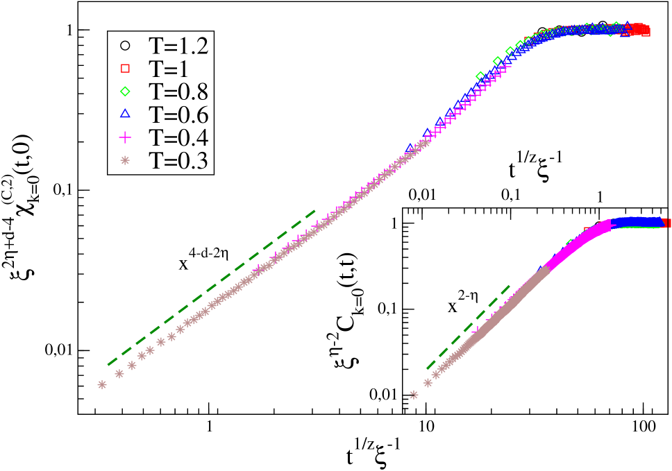
Figure 1: Data collapse of $\chi^{(c,2)}$ ($C$ in the inset) for several temperatures in the $d=1$ EA model. The dashed lines are the expected power-laws in the non equilibrium regime.

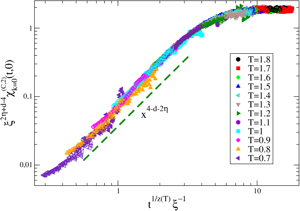
Figure 2: Data collapse of $\chi^{(c,2)}$ for several $T$ in the $d=2$ EA model with bimodal (open symbols)or Gaussian (filled symbols) bond distribution, with $z(T)=4/T$. The dashed line is the expected power-law in the non equilibrium regime.

In order to check these ideas and to test the efficiency of the method to measure the cooperative length we have computed numerically $\chi^{(c,2)}_{k=0}(t,0)$ in the Edwards-Anderson (EA) model with Hamiltonian $H=\sum_{ij}J_{ij}\sigma_{i}\sigma_{j}$ in $d\leq 2$, simulated by means of standard Montecarlo techniques, with Glauber transition rates, where $B_{i}=\sigma_{i}-\tanh(\beta\sum_{j}J_{ij}\sigma_{j})$. The system is quenched from a disordered state at $t=0$ to different final temperatures $T>0$. $\chi^{(c,2)}_{k=0}(t,0)$ is computed using Eq. (6). It must be stressed that, due to the noisy nature of response functions, the advantage provided by the FDR (6) instead of applying an infinitesimal perturbation is numerically un-renounceable. In fact, besides providing an incomparably better signal/noise ratio, the $h\to 0$ limit is built in the FDR. The analysis of the data proceeds as follows: from the large $t$ value $\chi^{(c,2)}_{k=0,eq}$ of $\chi^{(c,2)}$, knowing $\eta$, $\xi$ can be extracted for each temperature. Regarding $L(t)$, in the non-equilibrium regime $L(t)\ll\xi$, $\chi^{(c,2)}$ must be independent from $\xi$. Using (11) this implies $f(\xi/L(t),0)\sim(L(t)/\xi)^{4-d-2\eta}$. Hence the non-equilibrium behavior of $L(t)$ can also be determined. With these results, one can control that data collapse is obtained by plotting $\xi^{-4+d+2\eta}\chi^{(c,2)}_{k=0}(t,0)$ vs $L(t)/\xi$ for all the temperatures considered (see Figs. 1,2). We have studied first the model in $d=1$ with bimodal distribution of the coupling constants $J_{ij}=\pm 1$. This system can be considered as a laboratory since it can be mapped onto a ferromagnetic system where $\eta=1$ and $L(t)\sim t^{1/z}$, with $z=2$, are known analytically. Moreover, besides $\chi^{(c,2)}$, one can also check the scaling of the usual correlation $C_{k=0}(t,t)$ after the mapping and obtain another determination of $L(t)$ and $\xi$. In doing so, we find that the two methods to extract $L(t)$ and $\xi$ agree within the numerical uncertainty between them, and with the analytical behaviors. The data collapse of $\chi^{(c,2)}$ and of $C$ is shown in Fig. 1. Here one clearly observes the non-equilibrium kinetics in the early regime, characterized by a power-law behavior of $\chi^{(c,2)}$ with exponent $4-d-2\eta$, as expected, and the late equilibration with the convergence of $\chi^{(c,2)}_{k=0}(0,t)$ to $\chi^{(c,2)}_{k=0,eq}$. $C$ behaves similarly. After this explicit verification, we turn to the $d=2$ case, where the reference to $C$ is not available. In this case, with both bimodal and Gaussian distributions of $J_{ij}$, using $\eta=0$ sgd2bis , we find a behavior of $\xi$ consistent with previous results sgd2bis ; sgd2 . The non-equilibrium behavior is compatible with a power law $L(t)\sim t^{1/z(T)}$ with a temperature dependent exponent in agreement with $z(T)\simeq 4/T$, as reported in sgd2z . The data collapse of $\chi^{(c,2)}$ is shown in Fig. 2. Notice also the additional collapse of the curves with bimodal and Gaussian bond distribution, further suggesting that the two models may share the same universality class at finite temperatures sgd2bis .

In this Paper we have derived the exact beyond-linear FDR. The result, which can be straightforwardly extended to every order, provides a rather general relation between response and correlation functions: It is satisfied by systems described by a master equation or by a Langevin equation, without reference to specific aspects of the considered model. On the basis of the FDR we argued, providing numerical evidence, that the second order susceptibility $\chi^{(c,2)}$ is well fitted to uncover cooperative effects and to measure the coherence length in disordered and glassy systems. Importantly, this susceptibility has a simple operative definition, which might be fitted to experimental investigations. Finally, we mention that the relevance of the beyond-linear FDR is not restricted to the issue of cooperativity, but is related to a number of open questions among which the extension of the concept of effective temperatures beyond linear order.

References

(1)
L.F. Cugliandolo, J. Kurchan, and L. Peliti
Phys.Rev.E 55, 3898 (1997).
(2)
L.F. Cugliandolo and J. Kurchan, Phys.Rev.Lett. 71, 173 (1993);
J.Phys.A: Math.Gen. 27, 5749 (1994); Philos.Mag. 71, 501 (1995);
S. Franz, M. Mézard, G. Parisi and L. Peliti, Phys.Rev.Lett. 81, 1758
(1998); J.Stat.Phys. 97, 459 (1999).
(3)
L.F. Cugliandolo, J. Kurchan, and G. Parisi,
J.Phys. I France 4, 1641 (1994);
(4)
E. Lippiello, F. Corberi and M. Zannetti, Phys.Rev.E 71, 036104 (2005).
(5)
C. Donati, S.C. Glotzer and P. Poole, Phys.Rev.Lett. 82, 5064 (1999);
S. Franz, C. Donati, G. Parisi and S.C. Glotzer, Phil.Mag.B 79, 1827 (1999);
S. Franz and G. Parisi, J.Phys.:Condens.Mat. 12, 6335 (2000).
See also Ref. biroli for a discussion.
(6)
C. Toninelli, M. Wyart, L. Berthier, G. Biroli and J.P. Bouchaud,
Phys.Rev.E 71, 041505 (2005).
(7)
P. Mayer, H. Bissig, L. Berthier, L. Cipelletti, J.P. Garrahan, P. Sollich, and
V. Trappe, Phys.Rev.Lett. 93, 115701 (2004).
(8)
L. Berthier, G. Biroli, J.P. Bouchaud, L.Cipelletti, D. El Masri,
D. L Hôte,F. Ladieu and M. Pierno, Science 310, 1797 (2005).
(9)
G. Semerjian, L.F. Cugliandolo and A. Montanari, J.Stat.Phys. 115, 493 (2004).
(10)
J.P. Bouchaud and G. Biroli, Phys.Rev.B 72, 064204 (2005).
(11)
More details and higher order calculations will be presented elsewhere.
(12)
The FDR,
in the context of the
Langevin equation, has been derived also in biroli .
However, there are discrepancies between the results in biroli and ours.
The main ones are i) in the prefactors
involving and ii) in the contention made in biroli , which we do not agree with,
that the correlation functions with appearing with the shortest
time do vanish in equilibrium (see discussion below Eq. (11)).
(13)
T. J org, J. Lukic, E. Marinari and O.C. Martin, Phys.Rev.Lett. 96, 237205 (2006).
(14)
H.G. Katzgraber, L.W. Lee and A.P. Young, Phys. Rev. B 70, 014417 (2004);
H.G. Katzgraber, L.W. Lee and I.A. Campbell,
Phys.Rev.B 75, 014412 (2007).
(15)
H. Rieger, B. Steckemetz and M. Schreckenberg, Europhys. Lett. 27, 485 (1994);
H.G. Katzgraber, and I.A. Campbell, Phys.Rev.B 72, 014462 (2005).