High-statistics measurement of neutral-pion pair production in two-photon collisions

Abstract

We present a high-statistics measurement of differential cross sections and the total cross section for the process $\gamma\gamma\to\pi^{0}\pi^{0}$ in the kinematic range 0.6 GeV $\leq W\leq 4.0$ GeV and $|\cos\theta^{*}|\leq 0.8$, where $W$ and $\theta^{*}$ are the energy and pion scattering angle, respectively, in the $\gamma\gamma$ center-of-mass system. Differential cross sections are fitted to obtain information on S, D₀, D₂, G₀ and G₂ waves. The G waves are important above $W\simeq 1.6~{}{\rm GeV}$. General behavior of partial waves is studied by fitting differential cross sections in a simple parameterization where amplitudes contain resonant contributions and smooth background. The D₂ wave is dominated by the $f_{2}(1270)$ meson whose parameters are consistent with the with the current world averages. The D₀ wave contains a $f_{2}(1270)$ component, whose fraction is fitted. For the S wave, the $f_{0}(980)$ parameters are found to be consistent with the values determined from our recent $\pi^{+}\pi^{-}$ data. In addition to the $f_{0}(980)$, the S wave prefers to have another resonance-like contribution whose parameters are obtained.

The Belle Collaboration

I Introduction

Studies of exclusive hadronic final states in two-photon collisions give valuable information on the physics of light and heavy-quark resonances, perturbative and nonperturbative quantum chromodynamics (QCD) and hadron-production mechanisms. So far, Belle has measured the production cross sections of charged-pion pairs  bib:mori1 ; bib:mori2 ; bib:nkzw , charged- and neutral-kaon pairs bib:nkzw ; bib:kabe ; bib:wtchen , and proton-antiproton pairs bib:kuo . We have also analyzed $D$-meson-pair production finding a new charmonium state identified as the $\chi_{c2}(2P)$ bib:uehara .

Here we present the cross sections and an analysis of high-statistics neutral-pion pair production in two-photon processes. The motivation of this study is essentially the same as that for charged-pion pair production. However, the two processes are physically different and independent; we cannot predict one by measuring only the other.

In the low energy region ($W\stackrel{{\scriptstyle<}}{{\sim}}0.8$ GeV, where $W$ is the center-of-mass (c.m.) energy of the $\pi\pi$ system), it is expected that the difference of meson electric charges plays an essential role in the difference between the $\pi^{+}\pi^{-}$ and $\pi^{0}\pi^{0}$ cross sections. Predictions are not straightforward because of non-perturbative effects. In the intermediate energy range ($0.8~{}{\rm GeV}\stackrel{{\scriptstyle<}}{{\sim}}W\stackrel{{\scriptstyle<}}{{\sim}}2.4$ GeV), formation of meson resonances decaying to $\pi\pi$ is the dominant contribution. Since ordinary $q\bar{q}$ mesons conserve isospin in decays to $\pi\pi$, we can restrict the $I^{G}J^{PC}$ quantum numbers of the meson produced by two photons to be $0^{+}$(even)⁺⁺, that is, $f_{J={\rm even}}$ mesons. The ratio of the $f$-meson’s branching fractions, ${{\cal B}}(f\to\pi^{0}\pi^{0})/{{\cal B}}(f\to\pi^{+}\pi^{-})$ is 1/2 from isospin invariance. However, interference of resonances with the continuum component, which cannot be precisely calculated, distorts this ratio even near the resonant peaks.

A long-standing puzzle in QCD is the existence and structure of low mass ($\stackrel{{\scriptstyle<}}{{\sim}}1.5~{}{\rm GeV}/c^{2}$) scalar mesons bib:scalar . They, in particular, the $f_{0}(600)$ ($\sigma$ meson), are closely related to the QCD vacuum through spontaneous breakdown of chiral symmetry. Two-photon-resonant production of a meson gives valuable information such as its two-photon width, which is sensitive to its charge structure. Unfortunately, experimental constraints in a $B$ factory experiment do not allow measurements much below $W\stackrel{{\scriptstyle<}}{{\sim}}0.8$ GeV.

For higher energies ($W\stackrel{{\scriptstyle>}}{{\sim}}2.4~{}{\rm GeV}$), we can invoke a quark model. In leading order calculations bib:bl ; bib:bc which take into account spin correlations between quarks, the $\pi^{0}\pi^{0}$ cross section is predicted to be much smaller than that of $\pi^{+}\pi^{-}$, and the ratio of $\pi^{0}\pi^{0}$ to $\pi^{+}\pi^{-}$ is around 0.03-0.06. However, higher-order or nonperturbative QCD effects can modify this ratio. For example, the handbag model, which considers soft hadron exchange, predicts the same amplitude for the two processes and hence this ratio is expected to be 0.5 bib:handbag . Analyses of energy and angular distributions of the cross sections are essential to determine properties of the observed resonances and to test the validity of QCD models.

In this paper, we present measurements of the differential cross sections, $d\sigma/d|\cos\theta^{*}|$, for the process $\gamma\gamma\to\pi^{0}\pi^{0}$ in a wide two-photon c.m. energy ($W$) range from 0.6 to 4.0 GeV, in the c.m. angular range, $|\cos\theta^{*}|\leq 0.8$. The 95 fb^-1 data sample results in several hundred times larger statistics than in previous experiments bib:prev1 ; bib:prev2 . The data here are concentrated in the low energy region ($W\leq 1.6~{}{\rm GeV}$). In the higher energy region, many more resonances contribute and thus make an analysis based on a single experiment difficult. Furthermore, statistics are still poor in this range. The angular coverage up to $|\cos\theta^{*}|=0.8$ greatly enhances the capability for separating partial waves. In the low energy region, the cross section is dominated by the $f_{2}(1270)$. A clear peak corresponding to the $f_{0}(980)$ is found for the first time in two-photon production of $\pi^{0}\pi^{0}$. Furthermore, a “model-independent” partial wave analysis (where interference terms of amplitudes are temporarily neglected) reveals another resonance-like structure around 1.2 GeV in the S wave. This may be due to the contributions of the $f_{2}(1270)$ in the D₀ wave and/or scalar resonances such as the $f_{0}(1370)$. We fit the differential cross sections assuming such contributions and obtain their parameters.

This paper is organized as follows. In section II, the experimental apparatus relevant to this measurement is briefly described together with information on the trigger and a description of the event selection. Differential cross sections are derived in section III. In section  IV, the measured differential cross sections are fitted to obtain the resonance parameters of the $f_{0}(980)$ and a scalar meson as well as to extract the fraction of the $f_{2}(1270)$ in the D₀ wave. Finally in section V a summary and conclusion are given.

II Experimental Apparatus and Event Selection

We use data that corresponds to an integrated luminosity of 95 fb^-1 recorded with the Belle detector at the KEKB asymmetric-energy $e^{+}e^{-}$ collider bib:kekb . The $e^{+}e^{-}$ c.m. energy of the accelerator was set at 10.58 GeV (83 fb^-1), 10.52 GeV (9 fb^-1), 10.36 GeV ($\Upsilon(3S)$ runs, 2.9 fb^-1) and 10.30 GeV (0.3 fb^-1). The differences between the two-photon flux (luminosity function) in the measured $W$ regions due to differences in the beam energies are small (at most a few percent), and the fraction of integrated luminosity of the runs with lower beam energies is also small; we combine the results for different beam energies. The variation of the cross section because of this effect is less than 0.5%.

The Belle detector is a magnetic spectrometer covering a large solid angle (polar angles between $17^{\circ}$ and $150^{\circ}$ and the full azimuthal angle). A comprehensive description of the Belle detector is given elsewhere bib:belle . We mention here only those detector components that are essential to the present measurement. Charged tracks are reconstructed from hit information in a central drift chamber (CDC) located in a uniform 1.5 T solenoidal magnetic field. The $z$ axis of the detector and the solenoid are along the positron beam direction, with the positrons moving in the $-z$ direction. The CDC measures the longitudinal and transverse-momentum components (along the $z$ axis and in the $r\varphi$ plane, respectively). Photons are detected and measured in an electromagnetic calorimeter (ECL) located inside the solenoid. The ECL is an array of 8736 CsI(Tl) crystals pointing toward the interaction point, which help separating photons from $\pi^{0}$’s for energies up to $\simeq 4~{}{\rm GeV}$.

We require that there be no reconstructed CDC tracks coming from the vicinity of the nominal collision point. Photons from decays of two neutral pions are measured in the ECL. Signals from the ECL are used to trigger. The ECL trigger requirements are the following: the total ECL energy deposit in the triggerable acceptance region (see below) is greater than 1.15 GeV (the “HiE” trigger) or the number of ECL clusters (each crystal having more than 110 MeV) is four or greater (the “Clst4” trigger). The above energy thresholds are determined from a study of the correlations between the two triggers in data. This trigger logic is realized in hardware; no additional software filters are applied for events triggered by either of the two ECL triggers.

The analysis is performed in the “zero-tag” mode, where neither the recoil electron nor the positron is detected. We restrict the virtuality of the incident photons to be small by imposing strict transverse-momentum balance with respect to the beam axis for the final-state hadronic system.

The selection conditions for $\gamma\gamma\to\pi^{0}\pi^{0}$ signal candidates are the following. All the variables in criteria (1)-(6) are measured in the laboratory frame: (1) there is no good track that satisfies $dr<5$ cm, $dz<5$ cm and $p_{t}>0.1$ GeV/$c$, where $dr$ and $dz$ are the radial and axial distances, respectively, of closest approach (as seen in the $r\varphi$ plane) to the nominal collision point, and the $p_{t}$ is the transverse momentum measured in the laboratory frame with respect to the $z$ axis; (2) the events are triggered by either the HiE or Clst4 triggers; (3) there are two or more photons whose energies are greater than 100 MeV; (4) there are exactly two $\pi^{0}$’s, each $\pi^{0}$ having a transverse momentum greater than 0.15 GeV/$c$ with each of the decay-product photons having an energy greater than 70 MeV; (5) the two photons’ momenta are recalculated using a $\pi^{0}$-mass-constrained fit, and required to have a minimum $\chi^{2}$ value for the fit (there was a negligible fraction of events with ambiguous photon combinations); (6) the total energy deposit in the ECL is smaller than 5.7 GeV.

The transverse momentum in the $e^{+}e^{-}$ c.m. frame ($|\Sigma\mbox{\boldmath$p$}_{t}^{*}|$) of the two-pion system is then calculated. For further analysis, (7) we use events with $|\Sigma\mbox{\boldmath$p$}_{t}^{*}|<50$ MeV/$c$ as the signal candidates.

In order to reduce uncertainty from the efficiency of the hardware ECL triggers, we set offline selection criteria that emulate the hardware trigger conditions as follows: (8) the ECL energy sum within the triggerable region is greater than 1.25 GeV, or all four photons composing the two $\pi^{0}$ are contained in the triggerable acceptance region. Here, we define the triggerable acceptance region as the polar-angle ($\theta$) range in the laboratory system $17.0^{\circ}<\theta<128.7^{\circ}$.

III Derivation of Differential Cross Sections

In this section, we describe the derivation of differential cross sections. First, candidate events are divided into bins of $W$ and $|\cos\theta^{*}|$. Backgrounds are then subtracted by fitting the transverse-momentum distribution. Event distributions are unfolded to correct for finite energy resolution. Finally, differential cross sections are obtained in bins of $W$ and $|\cos\theta^{*}|$.

III.1 Signal Distributions

We derive the c.m. energy $W$ of the two-photon collision from the invariant mass of the two-neutral-pion system. We calculate the cosine of the scattering angle of $\pi^{0}$ in the $\gamma\gamma$ c.m. frame, $|\cos\theta^{*}|$. We then approximate the $e^{+}e^{-}$ collision axis in the $e^{+}e^{-}$ c.m. frame as the reference for this polar angle.

The two-dimensional yield distribution of the selected events is shown as a lego plot in Fig. 1. The $W$ distribution with $|\cos\theta^{*}|\leq 0.8$ is shown in Fig. 2. The total number of events observed is $1.25\times 10^{6}$. We observe clear peaks for the $f_{0}(980)$ near 0.98 GeV and the $f_{2}(1270)$ near 1.25 GeV and find at least two more structures around 1.65 GeV and 1.95 GeV.

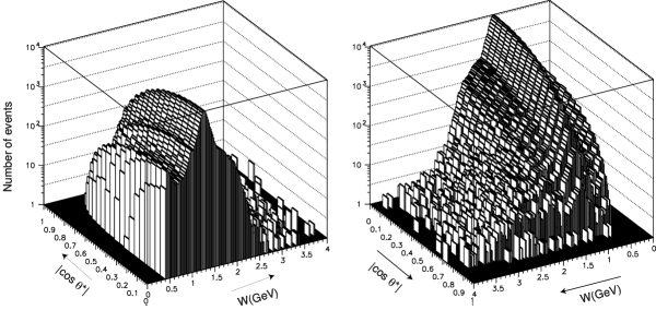
Figure 1: Two-dimensional $W$ and $|\cos\theta^{*}|$ distribution for $\pi^{0}\pi^{0}$ candidates in data. The same distribution is viewed from two different directions.

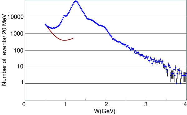
Figure 2: $W$ distribution for candidate events. The angular coverage is $|\cos\theta^{*}|\leq 0.8$. The curve is an estimate of backgrounds from events with $p_{t}$ imbalance (see text).

III.2 Background Subtraction

We use the $p_{t}$-balance distribution, i.e., the distribution in $|\Sigma\mbox{\boldmath$p$}_{t}^{*}|$, to separate the signal and background components. The signal Monte Carlo (MC) shows that the signal component peaks around 10-20 MeV/$c$ in this distribution. In the experimental data, however, in addition to the signal component, we find some contributions from $p_{t}$-unbalanced components in the low-$W$ region. Such $p_{t}$-unbalanced backgrounds might originate from processes such as $\pi^{0}\pi^{0}\pi^{0}$, etc. However, the background found in the experimental data is very large only in the low-$W$ region where the $\pi^{0}\pi^{0}\pi^{0}$ contribution is expected to be much smaller than $\pi^{0}\pi^{0}$ in two-photon collisions. (Note that a $C=-$ system cannot decay to $\pi^{0}\pi^{0}$.) We believe that the backgrounds are dominated by beam-background photons (or neutral pions from secondary interactions) or spurious hits in the detector.

Figures 3 (a) and (b) show the $p_{t}$-balance distributions in the low $W$ region. With the fit described below, we separate the signal components from the background. In the intermediate or higher energy regions, the $p_{t}$ unbalanced backgrounds are either less than 1%, buried under the $f_{2}(1270)$ peak (Fig. 3(c)), or consistent with zero within statistical errors. For the highest energy region 3.6 GeV$\leq W\leq 4.0$ GeV, we subtract a 3% background from the yield in each bin to account for the background from the $p_{t}$-unbalanced components and assign a systematic error of the same size, although it is not statistically significant even there (Fig. 3(d)).

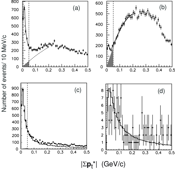
Figure 3: Distribution of imbalance in $|\sum\mbox{\boldmath$p$}^{*}_{t}|$ for candidate events. (a) In the bin centered at $W=0.90~{}$GeV and $|\cos\theta^{*}|=0.05$ (the bin width is 0.04 GeV and 0.1 in the $W$ and $|\cos\theta^{*}|$ directions, respectively, in (a)-(c)), the experimental distribution (dots with error bars) is fitted with the sum of signal and background components (curves). The gray region shows the estimated background contamination in the signal region. (b) The same as (a) for the bin centered at $W=0.66~{}$GeV. (c) In the $W=1.18$ GeV, $|\cos\theta^{*}|=0.65$ bin the experimental distribution is compared with the signal MC (histogram). (d) The same as (c) for $3.6~{}{\rm GeV}\leq W\leq 4.0$ GeV and $|\cos\theta^{*}|\leq 0.4$.

A fit to the $p_{t}$-balance distribution is performed in the region $|\sum\mbox{\boldmath$p$}_{t}^{*}|\leq 0.2~{}{\rm GeV}/c$ to separate the signal and background components for the $W$ region below 1.2 GeV. The fit function is a sum of the signal and background components. The signal component is an empirical function reproducing the shape of the signal MC, $y=Ax/(x^{2.1}+B+Cx)$, where $x\equiv|\sum\mbox{\boldmath$p$}_{t}^{*}|$, $A$, $B$ and $C$ are the fitting parameters, and $y$ is the distribution. This function has a peak at $x=(\frac{B}{1.1})^{\frac{1}{2.1}}$ and vanishes at $x=0$ and as $x\to\infty$. The shape of the background is taken as a linear function $y=ax$ for $x<0.05$ GeV/$c$, which is smoothly connected to a quadratic function above $x>0.05$ GeV/$c$.

The background yields obtained from the fits are fitted to a smooth two-dimensional function of ($W$, $|\cos\theta^{*}|$), in order not to introduce statistical fluctuations. The backgrounds are then subtracted from the experimental yield distribution. The background yields integrated over angle are shown in Fig. 2 for $W<1.2$ GeV. Above 1.2 GeV, we do not find any statistically significant background contributions from the fit. The correction and systematic errors from background are summarized in Sect. III.F. We omit the data points in the small-angle ($|\cos\theta^{*}|\geq 0.6$) region with $W\leq 0.72$ GeV, because there the background dominates the yield.

III.3 Unfolding the $W$ Distributions

We estimate the invariant-mass resolutions from studies of the signal MC and data. We find that the MC events have a relative invariant-mass resolution of 1.4%, which is almost constant over the entire $W$ region covered by the present measurement. The $\pi^{0}$ momentum resolution is known to be about 15% worse in the experimental data than in MC from a study of the $p_{t}$-balance distributions. Moreover, the distribution in the MC is asymmetric; it has a longer tail on the lower mass side. An asymmetric Gaussian function with standard deviations of 1.9%$W$ and 1.3%$W$ on the lower and higher sides of the peak, respectively, is used and approximates the smearing reasonably well. This invariant-mass resolution is comparable to or larger than the $W$ bin width (20 MeV) used in Figs. 1 and 2. We unfold the invariant-mass distribution in each $|\cos\theta^{*}|$ bin separately, to correct for migrations of signal yields to different $W$ bins in obtaining the true $W$ distribution, based on the asymmetric Gaussian smearing described above. The migration in the $|\cos\theta^{*}|$ direction is expected to be small and is neglected.

The unfolding uses the singular value decomposition algorithm bib:svdunf at the yield level and is applied so as to obtain the corrected $W$ distribution in the 0.9 - 2.4 GeV region, using data in the observed $W$ range between 0.72 and 3.0 GeV. For lower energies, $W\leq 0.9$ GeV, migration is expected to be small because of the better invariant-mass resolution compared with the bin width. For higher energies, $W>2.4$ GeV, where the statistics are relatively low and the unfolding would enlarge the errors, we rebin the data with a bin width of 100 MeV, instead of unfolding. Distributions before and after the unfolding for a typical angular bin ($|\cos\theta^{*}|=0.225$) are shown in Fig. 4.

We calibrate the experimental energy scale and invariant-mass distribution using the $\gamma\gamma$ invariant mass from experimental samples of $\eta^{\prime}\to\gamma\gamma$ in two-photon processes. The peak position is consistent with the nominal mass of $\eta^{\prime}$ with an accuracy better than 0.2%. The mass resolution estimated from the peak width is also consistent with the smearing function that is used for the unfolding of the $\pi^{0}\pi^{0}$ invariant-mass distributions.

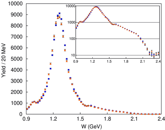
Figure 4: Invariant-mass distributions before (orange colored triangles) and after (dark-blue diamonds) the unfolding, at $|\cos\theta^{*}|=0.225$. The inset shows the same distribution on a semilogarithmic scale. The bin width changes from 0.02 GeV to 0.04 GeV above $W=1.6$ GeV.

III.4 Determination of Efficiency

We determine the efficiency for the signal using the detector and trigger simulators and applying the selection criteria to signal MC events. The $e^{+}e^{-}\to e^{+}e^{-}\pi^{0}\pi^{0}$ signal MC events are generated using the TREPS code bib:treps at 58 fixed $W$ points between 0.5 and 4.5 GeV, and isotropic in $|\cos\theta^{*}|$. The angular distribution at the generator level does not play a role in the efficiency determination, because we calculate the efficiencies separately in each 0.05 wide $|\cos\theta^{*}|$ bin. The number of events generated is $4\times 10^{5}$ at each $W$ point. To minimize statistical fluctuations in the MC calculation, we fit the efficiency to a two-dimensional empirical function in ($W$, $|\cos\theta^{*}|$). The efficiency thus determined is depicted in Fig. 5.

We find that the trigger efficiency, which is defined as the triggerable fraction of events that can pass through the event selection criteria, is almost flat and close to 100% for the region $W\stackrel{{\scriptstyle>}}{{\sim}}1.3$ GeV as shown in Fig. 6. It decreases to typically 30% at the lowest energies, $W<0.7$ GeV. Meanwhile, the overall efficiency (the product of the efficiencies for the trigger and the acceptance) is about 11% at maximum and decreases (down to around 1%) at lower $W$ or smaller c.m. angles (larger $|\cos\theta^{*}|$).

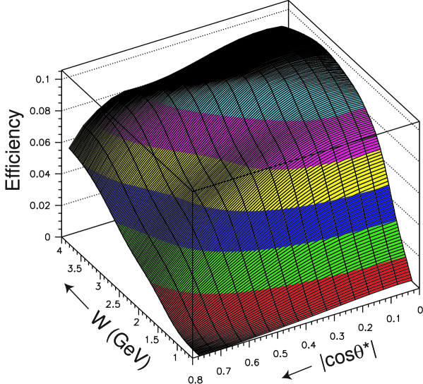
Figure 5: Overall efficiency in the $W-|\cos\theta^{*}|$ plane.

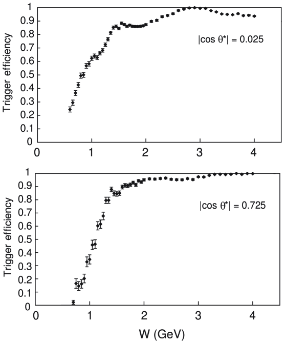
Figure 6: Trigger efficiencies plotted as a function of $W$ for two $|\cos\theta^{*}|$ bins.

The overall efficiency calculated using the signal MC events is corrected for a systematic difference found between the peak widths in the $p_{t}$-balance distributions of the experimental data and the MC, which could affect the efficiency through the $|\sum\mbox{\boldmath$p$}_{t}^{*}|$ cut. This originates from a difference in the momentum resolution for $\pi^{0}$’s between data and MC events. We find that the data peak position is 10% to 20% higher than the MC expectation, depending on $W$ and $|\cos\theta^{*}|$. The efficiency correction factor ranges from 0.90 to 0.95.

III.5 Cross-Section Calculation

The differential cross section for each ($W$, $|\cos\theta^{*}|$) point is derived from the following formula:

$$\frac{d\sigma}{d|\cos\theta^{*}|}=\frac{\Delta Y-\Delta B}{\Delta W\Delta|\cos\theta^{*}|\int{\cal L}dtL_{\gamma\gamma}(W)\eta}\;,$$ (1)

where $\Delta Y$ and $\Delta B$ are the signal yield and the estimated $p_{t}$-unbalanced background in each bin, $\Delta W$ and $\Delta|\cos\theta^{*}|$ are the bin widths, $\int{\cal L}dt$ and $L_{\gamma\gamma}(W)$ are the integrated luminosity and two-photon luminosity function calculated by TREPS, respectively, and $\eta$ is the net efficiency. The luminosity function transforms the cross sections for the $e^{+}e^{-}$ incident beam to that of the $\gamma\gamma$ incident using a relation:

$$L_{\gamma\gamma}(W)=\frac{d\sigma_{ee}}{dW}/\sigma_{\gamma\gamma}(W).$$

The $W$-bin width is 0.02 GeV up to 1.6 GeV and then is modified to 0.04 GeV and 0.1 GeV for $W$ between 1.6 GeV and 2.4 GeV and $W$ above 2.4 GeV, respectively. The width of the $|\cos\theta^{*}|$ bins are fixed to $\Delta|\cos\theta^{*}|=0.05$.

The differential cross sections obtained are shown at several $W$ points in Fig. 7. They show quite different behaviors. It should be noted that the cross-section results after the unfolding are no longer independent of each other in neighboring bins, in both central values and sizes of errors.

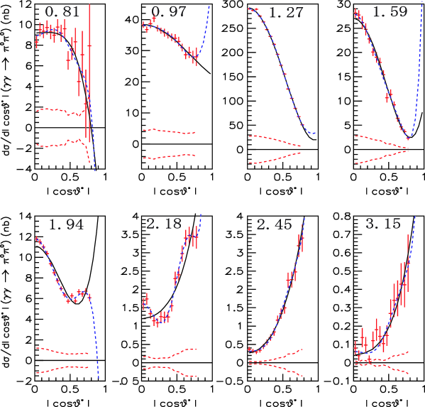
Figure 7: Differential cross sections for the eight selected $W$ points indicated in GeV in each figure. The results for $W\leq 2.4~{}{\rm GeV}$ are after the unfolding. The curves are fit results described in sec. IV; the solid (dashed) lines are the result of the $SD$ ($SDG$) fit (see text), while dotted lines indicate the size of systematic errors in the cross sections.

Figures 8(a) and (b) show the $W$ dependence of the cross section integrated over $|\cos\theta^{*}|\leq 0.8$ and $|\cos\theta^{*}|\leq 0.6$, respectively. They are obtained by adding $d\sigma/d|\cos\theta^{*}|\cdot\Delta|\cos\theta^{*}|$ over the corresponding angular bins. The total cross section ($|\cos\theta^{*}|\leq 0.8$) is dominated by the $f_{2}(1270)$. A clear peak due to the $f_{0}(980)$ is also visible as in the $\pi^{+}\pi^{-}$ cross section from Belle bib:mori1 ; bib:mori2 . Additional structures are visible around $W=1.65~{}{\rm GeV}$ and $W=1.95~{}{\rm GeV}$. The data points for $0.9~{}{\rm GeV}\leq W\leq 2.4~{}{\rm GeV}$ are the unfolded results where the bin widths $\Delta W$ are 0.02 GeV (0.04 GeV) in $W$ above (below) 1.6 GeV. For the data points above 2.4 GeV, we average five data points each with a bin width of 0.02 GeV and obtain results for every 0.1 GeV bin in $W$. We have removed the bins in the range 3.3 GeV $\leq W\leq 3.6$ GeV, because we cannot separate the contributions from $\chi_{c0}$, $\chi_{c2}$ and the continuum in a model-independent way, due to the finite mass resolution and insufficient statistics in this $W$ range.

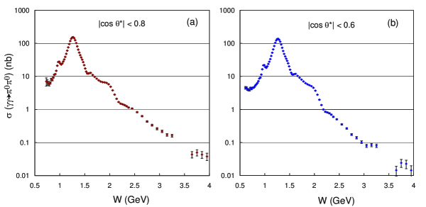
Figure 8: The total cross section for (a) $|\cos\theta^{*}|\leq 0.8$ and (b) $|\cos\theta^{*}|\leq 0.6$ after the unfolding and rebinning. See text for the bins in the range 3.3 GeV $\leq W\leq 3.6$ GeV.

III.6 Systematic Errors in the Cross Sections

We summarize the evaluation of the systematic errors for $\sigma(|\cos\theta^{*}|\leq 0.8)$ ($\sigma(|\cos\theta^{*}|\leq 0.6)$ for $W\leq 0.72$ GeV) at each $W$ point. These come from the following sources: trigger efficiency, reconstruction efficiency, $p_{t}$-balance cut, background subtraction, beam-background effect, other efficiency errors including smoothing procedure, unfolding procedure and luminosity function.

Trigger efficiency: the systematic error from the Clst4 trigger is assigned as $2/3$ of the difference of the efficiencies with different threshold assumptions for the ECL cluster – 110 MeV and 100 MeV – set in the trigger simulator for the energy region $W\leq 2.5$ GeV. We include a separate 4% uncertainty in the HiE trigger efficiency for the whole $W$ region. The systematic errors from the two triggers are added in quadrature. This systematic error becomes large in the low $W$ region, 20%-30% for $W\leq 0.8$ GeV.

Reconstruction efficiency: the uncertainty in the $\pi^{0}$ reconstruction efficiency is estimated from a comparison of $D^{0}$-meson decays to $K^{-}\pi^{+}$ and $K^{-}\pi^{+}\pi^{0}$. An error of 6% for two pions is assigned.

The $p_{t}$-balance cut is 3% - 5%, which is one half of the correction discussed above.

Background subtraction: 20% of the size of the subtracted component is assigned as the error from this source. In the $W$ region where the background subtraction is not applied ($W>1.2$ GeV), we neglect the error for 1.2 GeV$\leq W\leq 1.5$ GeV, and assign 3% for $W\geq 1.5$ GeV, which is an upper limit on the background contamination expected from the $p_{t}$-unbalanced distributions. For $W\geq 3.6$ GeV where we have applied a 3% correction for the background subtraction, we also assign a systematic error of the same magnitude.

Beam-background effect for event selection: we assign a 2% - 4% error depending on $W$ for uncertainties of the inefficiency in selection due to the effect of beam-background photons.

Other efficiency errors: an extra error of 4% is assigned for uncertainties in the efficiency determinations based on the MC including the smoothing procedure.

Unfolding procedure: we adopt the change in the unfolded yield in each bin when we modify the effective-rank parameter (kset parameter) applied in the unfolding procedure bib:svdunf in a reasonable range as a systematic error.

Luminosity function: the uncertainty is estimated to be 4% for $W<\;3.0$ GeV and 5% for $W>\;3.0$ GeV.

The total systematic error is 10% in the wide energy region, 1.0 GeV$\leq W\leq 3.4$ GeV. The error, which is dominated by the background subtraction, becomes much larger for lower $W$, 15% at $W=0.85$ GeV, 30% at $W=0.70$ GeV and 55% at $W=0.61$ GeV. For higher $W$, the systematic error is rather stable, remaining at the 11% level for 3.4 GeV$\leq W\leq 4.0$ GeV.

III.7 Comparison of Cross Sections with the Previous Experiment

The total cross section ($|\cos\theta^{*}|\leq 0.8$) is compared with the previous measurement by Crystal Ball at DORIS II bib:prev2 (Fig. 9). The agreement is fairly good. The error bars shown are statistical only, and the systematic errors (7% for $W>0.8~{}{\rm GeV}$ and 11% for $W<0.8~{}{\rm GeV}$ for the Crystal Ball results) should also be considered in the comparison. The present measurement has several hundred times more statistics than the Crystal Ball measurement.

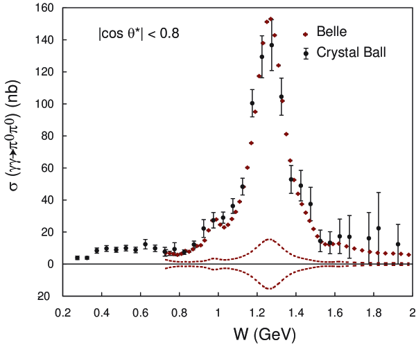
Figure 9: Cross section integrated over the angular region $|\cos\theta^{*}|\leq 0.8$ compared with the previous measurement from the Crystal Ball bib:prev2 . Dashed lines show the total systematic errors for the Belle measurement. Systematic errors of similar size (not shown) are present in the Crystal Ball measurement.

IV Fitting Differential Cross Sections

In this section, differential cross sections at each $W$ bin are fitted to obtain information on the partial waves. A simple parameterization is then fit to differential cross sections to obtain resonance parameters of the $f_{0}(980)$ and another scalar meson denoted here as $f_{0}(Y)$ as well as to extract the $f_{2}(1270)$ fraction in the D₀ wave.

IV.1 Formalism

In this channel, only partial waves of even angular momenta contribute. Furthermore, in the energy region $W\stackrel{{\scriptstyle<}}{{\sim}}3~{}{\rm GeV}$, $J>4$ partial waves (next is $J=6$) may be neglected so that only S, D and G waves are to be considered. The differential cross section can then be expressed as

$$\frac{d\sigma}{d\Omega}(\gamma\gamma\to\pi^{0}\pi^{0})=\left|S\>Y^{0}_{0}+D_{0}\>Y^{0}_{2}+G_{0}\>Y^{0}_{4}\right|^{2}+\left|D_{2}\>Y^{2}_{2}+G_{2}\>Y^{2}_{4}\right|^{2}\;,$$ (2)

where $D_{0}$ and $G_{0}$ ($D_{2}$ and $G_{2}$) denote the helicity 0 (2) components of the D and G waves, respectively, and $Y^{m}_{J}$ are the spherical harmonics:

$$Y^{0}_{0} = \sqrt{\frac{1}{4\pi}}\;,$$

$$Y^{0}_{2} = \sqrt{\frac{5}{16\pi}}(3\cos^{2}\theta^{*}-1)\;,$$

$$\left|Y^{2}_{2}\right| = \sqrt{\frac{15}{32\pi}}\sin^{2}\theta^{*}$$

$$Y^{0}_{4} = \frac{3}{16}\sqrt{\frac{1}{\pi}}(35\cos^{4}\theta^{*}-30\cos^{2}\theta^{*}+3)\;,$$

$$\left|Y^{2}_{4}\right| = \frac{3}{8}\sqrt{\frac{5}{2\pi}}(7\cos^{2}\theta^{*}-1)\sin^{2}\theta^{*}\;.$$ (3)

Since the $|Y^{m}_{J}|$s are not independent, partial waves cannot be separated using measurements of differential cross sections alone.

To overcome this problem, we begin by rewriting Eq. (2) as:

$$\frac{d\sigma}{4\pi d|\cos\theta^{*}|}(\gamma\gamma\to\pi^{0}\pi^{0})=\hat{S}^{2}\>|Y^{0}_{0}|^{2}+\hat{D}_{0}^{2}\>|Y^{0}_{2}|^{2}+\hat{D}_{2}^{2}\>|Y^{2}_{2}|^{2}\,+\hat{G}_{0}^{2}\>|Y^{0}_{4}|^{2}\,+\hat{G}_{2}^{2}\>|Y^{2}_{4}|^{2}\,.$$ (4)

The amplitudes $\hat{S}^{2}$, etc. correspond to the cases where interference terms are neglected. When interference terms are included, they can be written as (see Appendix A):

$$\hat{S}^{2} = |S|^{2}+\sqrt{5}\Re{(S^{*}D_{0})}-4\Re{(S^{*}G_{0})}+\frac{7}{\sqrt{5}}\Re{(D_{0}^{*}G_{0})}+\frac{14\sqrt{3}}{5}\Re{(D_{2}^{*}G_{2})}\;,$$

$$\hat{D}_{0}^{2} = |D_{0}|^{2}+\frac{1}{\sqrt{5}}\Re{(S^{*}D_{0})}+2\Re{(S^{*}G_{0})}+\frac{1}{\sqrt{5}}\Re{(D_{0}^{*}G_{0})}-\frac{4\sqrt{3}}{5}\Re{(D_{2}^{*}G_{2})}\;,$$

$$\hat{D}_{2}^{2} = |D_{2}|^{2}-\frac{6}{\sqrt{5}}\Re{(S^{*}D_{0})}+2\Re{(S^{*}G_{0})}+\sqrt{5}\Re{(D_{0}^{*}G_{0})}-\frac{9\sqrt{3}}{5}\Re{(D_{2}^{*}G_{2})}\;,$$

$$\hat{G}_{0}^{2} = |G_{0}|^{2}+\frac{3}{\sqrt{5}}\Re{(D_{0}^{*}G_{0})}+\frac{\sqrt{3}}{5}\Re{(D_{2}^{*}G_{2})}\;,$$

$$\hat{G}_{2}^{2} = |G_{2}|^{2}-\sqrt{5}\Re{(D_{0}^{*}G_{0})}-\frac{1}{\sqrt{3}}\Re{(D_{2}^{*}G_{2})}\;.$$ (5)

Since squares of spherical harmonics are independent of each other, we can fit differential cross sections at each $W$ to obtain $\hat{S}^{2}$, $\hat{D}_{0}^{2}$, $\hat{D}_{2}^{2}$, $\hat{G}_{0}^{2}$ and $\hat{G}_{2}^{2}$. The fit up to $J=4$ is called the “$SDG$ fit”. At low energy, we expect that $J=4$ waves are unimportant. Therefore we also perform a separate fit setting $\hat{G}_{0}^{2}=\hat{G}_{2}^{2}=0$, which is called the “$SD$ fit”.

The unfolded differential cross sections are fitted, where only statistical errors are taken into account in the fit. Although they are not independent at each $W$ because of the unfolding procedure, we treat them as independent in the fit. The effect of correlations between bins is taken into account in systematic errors as described below. Differential cross sections for $|\cos\theta^{*}|\leq 0.8$ are available for $0.73~{}{\rm GeV}\leq W\leq 4.0~{}{\rm GeV}$.

Examples of the fit quality are shown in Fig. 7. In the energy region near $W=2~{}{\rm GeV}$, a need for $J=4$ waves is evident. There, $\hat{G}_{2}^{2}$ deviates from zero as can be seen in Fig. 10. Since the behaviors of $|Y_{4}^{0}|^{2}$ and $|Y_{4}^{2}|^{2}$ are rather similar for $|\cos\theta^{*}|\stackrel{{\scriptstyle<}}{{\sim}}0.7$, we also fit with $|Y_{4}^{0}|^{2}\pm|Y_{4}^{2}|^{2}$. The bump in $\hat{G}_{0}^{2}+\hat{G}_{2}^{2}$ may indicate the presence of the $f_{4}(2050)$. However, in the high energy region $W>1.6$ GeV, there are many more resonances contributing and thus the model uncertainty becomes much larger. Therefore in this paper we focus on the energy region $0.8~{}{\rm GeV}\leq W\leq 1.6~{}{\rm GeV}$, where G waves can be neglected. The $\hat{S}^{2}$, $\hat{D}_{0}^{2}$ and $\hat{D}_{2}^{2}$ spectra are shown in Fig. 11.

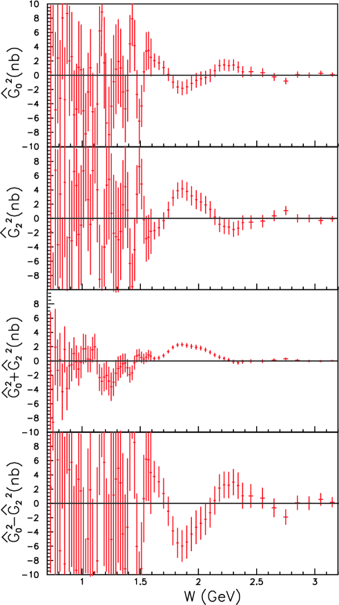
Figure 10: The $\hat{G}_{0}^{2}$, $\hat{G}_{2}^{2}$ and $\hat{G}_{0}^{2}\pm\hat{G}_{2}^{2}$ spectra for the $SDG$ fit.

Figure 11: The $\hat{S}^{2}$ (top), $\hat{D}_{0}^{2}$ (middle) and $\hat{D}_{2}^{2}$ (bottom) spectra. Curves are result of the fit with the parameterization discussed in text. The error bars are diagonal statistical errors only.

IV.2 Fitting Partial Wave Amplitudes

In this section, we derive some information on the relevant resonances by fitting differential cross sections by assuming certain functional forms for the partial wave amplitudes to understand the general behavior of partial wave amplitudes and to check the consistency with the $\pi^{+}\pi^{-}$ data bib:mori1 ; bib:mori2 . Note that we do not fit the obtained $\hat{S}^{2}$, etc. but fit the differential cross sections directly; once the functional forms of amplitudes are assumed, we can use Eq. (2) to fit differential cross sections.

Here, we concentrate on the energy region $W\leq 1.6~{}{\rm GeV}$, where G₀ and G₂ can be neglected. A full amplitude analysis will be performed in the near future using all data available in addition to the $\pi^{0}\pi^{0}$ data. Thus we employ a simple parameterization in this study. The $\hat{D}_{2}^{2}$ spectrum is dominated by the $f_{2}(1270)$ resonance. The $f_{2}(1270)$ could contribute to the D₀ wave. The $\hat{S}^{2}$ distribution has peaks apparently due to the $f_{0}(980)$ resonance and another resonance-like structure around 1.2 GeV, which motivates us to introduce a scalar meson denoted here as $f_{0}(Y)$ together with a contribution from the $f_{2}(1270)$ in the D₀ wave. The $f_{0}(Y)$ can be either the $f_{0}(1370)$ or $f_{0}(1500)$ or a mixture of both bib:PDG . Note that the mass and width of the $f_{0}(1370)$ are known with a large uncertainty bib:PDG . Neither of these states has been observed previously in two-photon production bib:aleph . The goal of this analysis is to obtain parameters of the $f_{0}(980)$ and $f_{0}(Y)$, to check the consistency of the $f_{2}(1270)$ parameterization where its two-photon branching fraction is floated and to measure the helicity 0-to-helicity 2 ratio of $f_{2}(1270)$ production.

IV.2.1 Parameterization of Amplitudes

Based on the above observations, the S, D₀ and D₂ waves are parameterized as follows:

$$S = A_{f_{0}(980)}e^{i\phi_{s0}}+A_{f_{0}(Y)}e^{i\phi_{s1}}+B_{S},$$

$$D_{0} = \sqrt{\frac{r_{02}}{1+r_{02}}}A_{f_{2}(1270)}e^{i\phi_{d0}}+B_{D0},$$

$$D_{2} = \sqrt{\frac{1}{1+r_{02}}}A_{f_{2}(1270)}e^{i\phi_{d2}}+A_{f_{2}^{\prime}(1525)}e^{i\phi_{d2^{\prime}}}+B_{D2},$$ (6)

where $A_{f_{0}(980)}$, $A_{f_{0}(Y)}$, $A_{f_{2}(1270)}$ and $A_{f_{2}^{\prime}(1525)}$ are the amplitudes of the $f_{0}(980)$, another scalar resonance denoted as $f_{0}(Y)$, the $f_{2}(1270)$ and the $f_{2}^{\prime}(1525)$, respectively; $B_{S}$, $B_{D0}$ and $B_{D2}$ are “background” amplitudes for S, D₀ and D₂ waves; and $\phi_{s0}$, $\phi_{s1}$, $\phi_{d0}$, $\phi_{d2}$ and $\phi_{d2^{\prime}}$ are the phases of resonances relative to background amplitudes. The parameter $r_{02}$ represents the fraction of the $f_{2}(1270)$ component in the D₀ wave. Here, as a default, we assume the presence of both the $f_{0}(Y)$ in the S wave and the $f_{2}(1270)$ in the D₀ wave. We also study the cases where either $r_{02}=0$ or there is no $f_{0}(Y)$.

We assume background amplitudes to be quadratic in $W$ for all the waves:

$$B_{S} = a_{sr}W^{2}+b_{sr}W+c_{sr}+i(a_{si}W^{2}+b_{si}W+c_{si}),$$

$$B_{D0} = a_{0}W^{2}+b_{0}W+c_{0},$$

$$B_{D2} = a_{2}W^{2}+b_{2}W+c_{2}.$$ (7)

The $D_{0}$ and $D_{2}$ background amplitudes are taken to be real by definition.

We use the parameterization of the $f_{0}(980)$, $f_{2}(1270)$ and $f_{2}^{\prime}(1525)$ given in Ref. bib:mori1 and bib:mori2 . We note that ${{\cal B}}(f_{J}\rightarrow\pi^{0}\pi^{0})/{{\cal B}}(f_{J}\rightarrow\pi^{+}\pi^{-})=1/2$ (because the $f_{J}$ mesons are isoscalars). For completeness, we reproduce the parameterization of the $f_{0}(980)$ and $f_{2}(1270)$. For the $f_{0}(980)$ meson, we take

$$A_{f_{0}(980)}=\frac{\sqrt{8\pi\beta_{\pi}}}{W}\frac{g_{f_{0}\gamma\gamma}g_{f_{0}\pi\pi}}{16\pi}\cdot\frac{1}{D_{f_{0}}},$$ (8)

where $\beta_{X}=\sqrt{1-\frac{4{M_{X}}^{2}}{W^{2}}}$ is the velocity of the particle $X$ with mass $M_{X}$ in the two-body final states, $g_{f_{0}XX}$ is related to the partial width of the $f_{0}(980)$ meson via $\Gamma_{XX}(f_{0})=\frac{\beta_{X}g_{f_{0}XX}^{2}}{16\pi M_{f_{0}}}$. The factor $D_{f_{0}}$ is given as follows bib:denom :

$$D_{f_{0}}(W)=M_{f_{0}}^{2}-W^{2}+\Re{\Pi_{\pi}^{f_{0}}}\left(M_{f_{0}}\right)-\Pi_{\pi}^{f_{0}}\left(W\right)+\Re{\Pi_{K}^{f_{0}}}\left(M_{f_{0}}\right)-\Pi_{K}^{f_{0}}\left(W\right),$$

where for $X=\pi$ or $K$,

$$\Pi_{X}^{f_{0}}(W)=\frac{\beta_{X}{g^{2}_{f_{0}XX}}}{16\pi}\left[i+\frac{1}{\pi}\ln\frac{1-\beta_{X}}{1+\beta_{X}}\right].$$ (9)

The factor $\beta_{K}$ is real in the region $W\geq 2M_{K}$ and becomes imaginary for $W<2M_{K}$. The mass difference between $K^{\pm}$ and $K^{0}$ $(\overline{K^{0}})$ is included by using $\beta_{K}=\frac{1}{2}(\beta_{K^{\pm}}+\beta_{K^{0}})$. The parameters assumed and determined in Ref. bib:mori1 are summarized in Table 1.

Table 1: Parameters of the $f_{0}\left(980\right)$ assumed and fitted in Ref. bib:mori1 .

Parameter	Value	Unit	Reference
Mass	$985.6~{}^{+1.2}_{-1.5}\left(\rm stat\right)~{}^{+1.1}_{-1.6}\left(\rm syst\right)$	${\rm MeV}/c^{2}$	bib:mori1
$g_{f_{0}(980)\pi\pi}$	$1.33~{}_{-0.23}^{+0.27}\left(\rm stat\right)~{}_{-0.05}^{+0.16}\left(\rm syst\right)$	GeV	bib:mori1
$\Gamma_{\pi^{+}\pi^{-}}$	$34.2~{}^{+13.9}_{-11.8}\left(\rm stat\right)~{}^{+8.8}_{-2.5}\left(\rm syst\right)$	MeV	bib:mori1
$g^{2}_{f_{0}(980)KK}/g^{2}_{f_{0}(980)\pi\pi}$	$4.21~{}\pm 0.25\left(\rm stat\right)~{}\pm 0.21\left(\rm syst\right)$	–	bib:bes
$\Gamma_{\gamma\gamma}$	$205~{}^{+95}_{-83}\left(\rm stat\right)~{}^{+147}_{-117}\left(\rm syst\right)$	eV	bib:mori1

Next, we give the parameterizations of the $f_{2}(1270)$ and $f_{2}^{\prime}(1525)$ mesons. The relativistic Breit-Wigner resonance amplitude $A_{R}(W)$ for a spin-$J$ resonance $R$ of mass $m_{R}$ is given by

$$A_{R}^{J}(W) = \sqrt{\frac{8\pi(2J+1)m_{R}}{W}}\times\frac{\sqrt{\Gamma_{\gamma\gamma}(W)\Gamma_{\pi^{0}\pi^{0}}(W)}}{m_{R}^{2}-W^{2}-im_{R}\Gamma_{\rm tot}(W)}\;,$$ (10)

Hereafter we consider the case $J=2$ (the $f_{2}(1270)$ and $f_{2}^{\prime}(1525)$ mesons). The energy-dependent total width $\Gamma_{\rm tot}(W)$ is given by

$$\Gamma_{\rm tot}(W)=\sum_{X}\Gamma_{X\bar{X}}(W)\;,$$ (11)

where $X$ is $\pi$, $K$, $\gamma$, etc. The partial width $\Gamma_{X\bar{X}}(W)$ is parameterized as bib:blat

$$\Gamma_{X\bar{X}}(W)=\Gamma_{R}{\cal B}(R\rightarrow X\bar{X})\left(\frac{q_{X}(W^{2})}{q_{X}(m_{R}^{2})}\right)^{5}\frac{D_{2}\left(q_{X}(W^{2})r_{R}\right)}{D_{2}\left(q_{X}(m_{R}^{2})r_{R}\right)}\;,$$ (12)

where $\Gamma_{R}$ is the total width at the resonance mass, $q_{X}(W^{2})=\sqrt{W^{2}/4-m_{X}^{2}}$, $D_{2}(x)=1/(9+3x^{2}+x^{4})$, and $r_{R}$ is an effective interaction radius that varies from 1 $({\rm GeV}/c)^{-1}$ to 7 $({\rm GeV}/c)^{-1}$ in different hadronic reactions bib:grayer . For the $4\pi$ and the other decay modes, $\Gamma_{4\pi}(W)=\Gamma_{R}{\cal B}(R\rightarrow 4\pi)\frac{W^{2}}{m_{R}^{2}}$ is used instead of Eq. (12). In Ref. bib:mori2 , all parameters of the $f_{2}(1270)$ are fixed at the PDG values bib:PDG , except for $r_{R}$, as summarized in Table 2.

In the fit below, we float the branching fraction of the $f_{2}(1270)$ into two photons, because its value determined in the past experiments is based on various assumptions.

Table 2: Parameters of the $f_{2}\left(1270\right)$ and $f_{2}^{\prime}\left(1525\right)$ assumed

Parameter	$f_{2}(1270)$	$f_{2}^{\prime}(1525)$	Unit	Reference
Mass	$1275.4\pm 1.1$	$1525\pm 5$	${\rm MeV}/c^{2}$	bib:PDG
$\Gamma_{\rm tot}$	$185.2^{+3.1}_{-2.5}$	$73^{+6}_{-5}$	MeV	bib:PDG
${\cal B}({f_{2}\rightarrow\pi\pi})$	$84.8^{+2.5}_{-1.3}$	$0.82\pm 0.15$	%	bib:PDG
${\cal B}({f_{2}\rightarrow K\bar{K}})$	$4.6\pm 0.4$	$88.8\pm 3.1$	%	bib:PDG
${\cal B}({f_{2}\rightarrow\eta\eta})$	–	$10.3\pm 3.1$	%	bib:PDG
${\cal B}({f_{2}\rightarrow\gamma\gamma})$	$14.1\pm 1.3$	$1.11\pm 0.14$	$\times 10^{-6}$	bib:PDG
$r_{R}$	$3.62\pm 0.03$		$({\rm GeV}/c)^{-1}$	bib:mori2

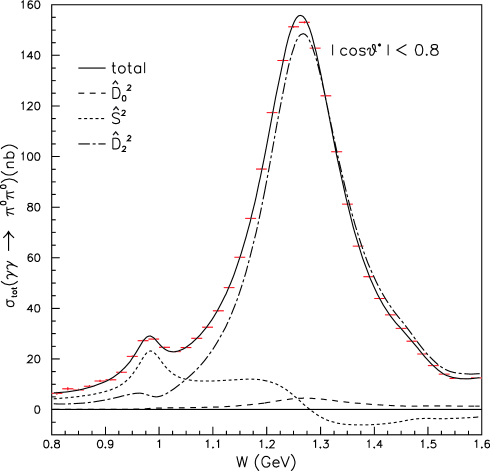
Figure 12: Total cross section ($|\cos\theta^{*}|\leq 0.8$) and results of parameterization. Contributions of $\hat{S}^{2},\;\hat{D}_{0}^{2}$ and $\hat{D}_{2}^{2}$ are also shown.

Finally, the parameterization of the $f_{0}(Y)$ meson is taken to be:

$$A_{f_{0}(Y)}=\sqrt{\frac{8\pi m_{f_{0}(Y)}}{W}}\frac{\sqrt{\Gamma_{f_{0}(Y)}\Gamma_{\gamma\gamma}(f_{0}(Y)){\cal B}(f_{0}(Y)\to\pi^{0}\pi^{0})}}{m^{2}_{f_{0}(Y)}-W^{2}-im_{f_{0}(Y)}\Gamma_{f_{0}(Y)}}\;,$$ (13)

where $\Gamma_{\gamma\gamma}(f_{0}(Y))$ is the two-photon width of the $f_{0}(Y)$ meson.

IV.2.2 Fitted Parameters

We fit differential cross sections with the parameterized amplitudes in the c.m. energy range 0.8 GeV$\leq W\leq$ 1.6 GeV. The parameter $g^{2}_{KK}/g^{2}_{\pi\pi}$ for the $f_{0}(980)$ is fixed to zero because this is preferred by the fit with a large error. There are 25 parameters to be fitted. The coefficients $a_{0}$ and $a_{2}$ in the continuum parameterizations are chosen to be positive to fix sign ambiguities. About 3000 sets of randomly generated initial parameters are prepared and fitted using MINUIT bib:minuit to search for the true minimum and to find any multiple solutions. Once solutions are found, several tens of MINUIT iterations are needed for convergence; with many parameters (25 here and $21-26$ for later analyses); the approach to the minimum is rather slow. A unique solution is found with $\chi^{2}/ndf=1010.1/615=1.64$ for the nominal fit, where $ndf$ is the number of degrees of freedom. The fitted parameters are listed in Table 3. The errors quoted are statistical only. The fit quality is adequate, $\chi^{2}/ndf=1.64$, and represents the trend of the squared amplitudes as shown in Fig. 11. The error bars in the figure are diagonal statistical errors only. The quantity $\hat{D}_{2}^{2}$ is well reproduced except below 1.1 GeV. The effect of the $f_{2}^{\prime}(1525)$ is rather small and not visible in the figures. Additional assumptions or a more complicated model are needed to better reproduce the structures visible in $\hat{D}_{0}^{2}$ for the range $1.1~{}{\rm GeV}\stackrel{{\scriptstyle<}}{{\sim}}W\stackrel{{\scriptstyle<}}{{\sim}}1.4~{}{\rm GeV}$ (the $f_{2}(1270)$ region).

Table 3: Fitted parameters

Parameter	Nominal	$r_{02}=0$	No $f_{0}(Y)$	Unit
Mass(${f_{0}(980)})$	$982.2\pm 1.0$	$980.2\pm 1.0$	$983.7^{+1.5}_{-1.0}$	MeV/$c^{2}$
$\Gamma_{\gamma\gamma}(f_{0}(980))$	$285.5^{+17.2}_{-17.1}$	$297.0^{+14.2}_{-13.7}$	$370.5^{+20.2}_{-18.7}$	eV
$g_{f_{0}(980)\pi\pi}$	$1.82\pm 0.03$	$1.79\pm 0.03$	$1.89\pm 0.03$	GeV
Mass($f_{0}(Y))$	$1469.7\pm 4.7$	$1466.8\pm 0.6$	–	MeV/$c^{2}$
$\Gamma(f_{0}(Y))$	$89.7^{+8.1}_{-6.6}$	$422.4^{+18.4}_{-19.8}$	–	MeV
$\Gamma_{\gamma\gamma}{\cal B}(f_{0}(Y)\to\pi^{0}\pi^{0})$	$11.2^{+5.0}_{-4.0}$	$6780.2^{+626.5}_{-574.7}$	0 (fixed)	eV
$r_{02}$	$3.69^{+0.24}_{-0.29}$	0 (fixed)	$5.04^{+0.26}_{-0.24}$	%
${\cal B}(f_{2}(1270)\rightarrow\gamma\gamma)$	$1.57\pm 0.01$	$1.62^{+0.02}_{-0.01}$	$1.52^{+0.13}_{-0.31}$	$\times 10^{-5}$
$\chi^{2}\;(ndf)$	1010.1 (615)	1206.1 (617)	1253.3 (619)

The total cross section ($|\cos\theta^{*}|\leq 0.8$) can be obtained by integrating Eq. (4) as

$$\sigma_{\rm tot}=0.8\hat{S}^{2}+0.45728\hat{D}_{0}^{2}+0.988288\hat{D}_{2}^{2}\;,$$ (14)

where the numerical factors come from the integration of spherical harmonics for $|\cos\theta^{*}|\leq 0.8$. The measured total cross section is compared with the prediction obtained from the fitted amplitudes as shown in Fig. 12. They are reproduced reasonably well.

So far we assumed a need for both the $f_{0}(Y)$ in the S wave and the $f_{2}(1270)$ in the D₀ wave ($r_{02}\neq 0$). We also study cases where either one of them is absent. One thousand sets of randomly generated initial values are prepared and fitted to find the true minimum. Unique solutions are found in each case. The values obtained are also listed in Table 3. The $\chi^{2}/ndf$ clearly favors the presence of both components.

Comparing the case of no $f_{0}(Y)$ and no $f_{2}(1270)$ in the D₀ wave, the fit prefers the latter: $\chi^{2}/ndf=1206.1/617$ compared to $1253.3/619$. Thus we conclude that the possibility of only the $f_{2}(1270)$ in the D₀ wave is disfavored compared to the case of only the $f_{0}(Y)$ in the S wave by more than 6 standard deviations, which is calculated from the difference of the $\chi^{2}$ taking the difference of $ndf$s into account.

IV.2.3 Study of Systematic Errors

The following sources of systematic errors on the parameters are considered: dependence on the fitted region, normalization errors in the differential cross sections, assumptions on the background amplitudes, uncertainties from the unfolding procedure, uncertainties in the parameters assumed for the $f_{0}(980)$ and uncertainties in the measurements of the $f_{2}(1270)$ and $f_{2}^{\prime}(1525)$.

In each study, a fit is made allowing all the parameters to float and the differences of the fitted parameters from the nominal values are quoted as systematic errors. One thousand sets of randomly generated input parameters are again prepared for each study and fitted to search for the true minimum and for possible multiple solutions. Unique solutions are found in each case.

Two fitting regions are tried: a narrow one ($0.84~{}{\rm GeV}\leq W\leq 1.56~{}{\rm GeV}$) and a wide one ($0.76~{}{\rm GeV}\leq W\leq 1.64~{}{\rm GeV}$). Normalization error studies are divided into those from uncertainties of the overall normalization and those from smearing of the spectra in either $|\cos\theta^{*}|$ or $W$. For overall normalization errors, fits are made with two sets of values of differential cross sections obtained by multiplying by $(1\pm\sigma_{\epsilon(W,|\cos\theta^{*}|)})$, where $\sigma_{\epsilon}$ is the relative efficiency error. For smearing studies, $\pm 4$% errors are assigned and differential cross sections are smeared by $(1\pm 0.1|\cos\theta^{*}|\mp 0.04)$ and $(1\pm 0.1W\mp 0.12)$.

For studies of background (BG) amplitudes, one of the waves is changed to either a first- or a third-order polynomial. In estimating uncertainties from the unfolding procedure, the kset parameter bib:svdunf is varied by $\pm 4$ from its nominal value. When this parameter is increased, the constraints between adjacent bins become weaker and oscillating solutions tend to appear as the statistical errors increase. When kset decreases, the opposite trend occurs.

For the parameterization of the $f_{0}(980)$, the fit prefers zero for the ratio $g^{2}_{KK}/g^{2}_{\pi\pi}$ as stated above and hence we set the ratio to be zero in the nominal fit. A systematic error due to this assumption is studied by setting the ratio to be 4.45, a value 1 standard deviation larger according to the BES measurement bib:bes . Finally, the $f_{2}(1270)$ and $f_{2}^{\prime}(1525)$ parameters are varied by their errors.

The resulting systematic errors are summarized in Table 4. It is noted that the mass of the $f_{0}(Y)$ jumps from $\sim 1.5~{}{\rm GeV}/c^{2}$ to $\sim 1.2~{}{\rm GeV}/c^{2}$, which is “compensated” by an increased value of $r_{02}$ in a systematic error study on unfolding. There, the change of cross-section values from the nominal ones is rather small (at most 15% at $|\cos\theta^{*}|\simeq 0.8$) with some systematic dependence on $\cos\theta^{*}$ in some $W$ bins, showing the sensitive nature of this kind of analysis. Total systematic errors are calculated by adding individual errors in quadrature.

Table 4: Systematic uncertainties for $f_{0}$ and $f_{2}$ parameters

	$f_{0}(980)$			$f_{0}(Y)$
Source	Mass	$\Gamma_{\gamma\gamma}$	$g_{\pi\pi}$	Mass	$\Gamma_{\rm tot}$	$\Gamma_{\gamma\gamma}{\cal B}_{\pi^{0}\pi 0}$	$r_{02}$	${\cal B}(f_{2}\rightarrow\gamma\gamma)$
	(MeV/$c^{2}$)	(eV)	(GeV)	(MeV/$c^{2}$)	(MeV)	(eV)	(%)	$(\times 10^{-5})$
$W$-range	${}^{+0.0}_{-2.8}$	${}^{+118.8}_{-0.0}$	${}^{+0.10}_{-0.02}$	${}^{+30.0}_{-49.7}$	${}^{+1.4}_{-13.0}$	${}^{+7.5}_{-5.0}$	${}^{+0.51}_{-0.00}$	${}^{+0.57}_{-0.00}$
Normalization	${}^{+0.6}_{-0.4}$	${}^{+0.0}_{-28.5}$	${}^{+0.00}_{-0.01}$	${}^{+8.8}_{-0.0}$	${}^{+15.0}_{-3.2}$	${}^{+10.5}_{-1.5}$	${}^{+0.29}_{-1.61}$	${}^{+0.44}_{-0.14}$
Bias:$|\cos\theta^{*}|$	${}^{+0.0}_{-1.0}$	${}^{+6.9}_{-28.9}$	${}^{+0.00}_{-0.02}$	${}^{+16.0}_{-0.0}$	${}^{+13.1}_{-0.0}$	${}^{+8.5}_{-0.0}$	${}^{+0.00}_{-1.09}$	${}^{+0.38}_{-0.00}$
Bias:$W$	${}^{+0.1}_{-2.2}$	${}^{+10.8}_{-0.0}$	${}^{+0.00}_{-0.01}$	${}^{+25.8}_{-2.5}$	${}^{+1.0}_{-2.4}$	${}^{+8.2}_{-0.3}$	${}^{+0.01}_{-0.15}$	${}^{+0.58}_{-0.01}$
BG:$\Re(S)$	${}^{+0.0}_{-1.3}$	${}^{+127.1}_{-9.3}$	$\pm 0.02$	${}^{+6.8}_{-19.5}$	${}^{+0.3}_{-3.1}$	${}^{+2.2}_{-3.8}$	${}^{+1.14}_{-1.66}$	${}^{+0.07}_{-0.01}$
BG:$\Im(S)$	${}^{+0.0}_{-2.5}$	${}^{+35.3}_{-0.0}$	${}^{+0.00}_{-0.01}$	${}^{+19.8}_{-0.0}$	${}^{+0.0}_{-7.6}$	${}^{+0.8}_{-0.6}$	${}^{+2.52}_{-0.00}$	${}^{+0.02}_{-0.01}$
BG:$D_{0}$	${}^{+0.1}_{-2.6}$	${}^{+30.6}_{-5.3}$	${}^{+0.01}_{-0.00}$	${}^{+27.1}_{-2.2}$	${}^{+1.3}_{-1.7}$	${}^{+8.4}_{-0.5}$	${}^{+0.26}_{-0.62}$	${}^{+0.59}_{-0.00}$
BG:$D_{2}$	${}^{+0.0}_{-2.9}$	${}^{+30.7}_{-0.0}$	${}^{+0.01}_{-0.00}$	${}^{+42.6}_{-0.0}$	${}^{+6.3}_{-10.6}$	${}^{+10.0}_{-0.0}$	${}^{+0.00}_{-0.38}$	${}^{+0.51}_{-0.00}$
Unfolding	${}^{+0.0}_{-5.0}$	${}^{+2.4}_{-48.5}$	${}^{+0.22}_{-0.16}$	${}^{+0.0}_{-249.5}$	${}^{+39.6}_{-0.0}$	${}^{+602.9}_{-0.0}$	${}^{+15.63}_{-0.37}$	${}^{+0.33}_{-0.00}$
$g_{KK}\neq 0$	${}^{+8.0}_{-0.0}$	${}^{+97.4}_{-0.0}$	${}^{+0.00}_{-0.02}$	${}^{+10.5}_{-0.0}$	${}^{+12.7}_{-0.0}$	${}^{+11.1}_{-0.0}$	${}^{+0.00}_{-0.91}$	${}^{+0.46}_{-0.00}$
$f_{2}$:mass	${}^{+0.1}_{-0.7}$	${}^{+26.5}_{-26.6}$	${}^{+0.02}_{-0.03}$	${}^{+5.1}_{-3.8}$	${}^{+12.3}_{-10.7}$	${}^{+5.7}_{-2.9}$	${}^{+0.36}_{-0.21}$	${}^{+0.00}_{-0.01}$
$f_{2}$:width	${}^{+0.6}_{-1.2}$	${}^{+3.9}_{-2.8}$	${}^{+0.00}_{-0.01}$	${}^{+11.7}_{-10.3}$	${}^{+2.6}_{-0.5}$	${}^{+1.5}_{-0.0}$	${}^{+0.13}_{-0.11}$	${}^{+0.01}_{-0.02}$
$f_{2}:{\cal B}(\pi\pi)$	${}^{+0.0}_{-0.1}$	${}^{+0.7}_{-0.0}$	$\pm 0.00$	${}^{+0.4}_{-0.0}$	${}^{+1.7}_{-0.0}$	${}^{+0.7}_{-0.0}$	${}^{+0.00}_{-0.07}$	${}^{+0.02}_{-0.00}$
$f_{2}:{\cal B}(KK)$	${}^{+0.0}_{-0.3}$	${}^{+4.0}_{-8.7}$	${}^{+0.00}_{-0.01}$	${}^{+1.8}_{-0.0}$	${}^{+2.5}_{-0.0}$	${}^{+1.4}_{-0.1}$	${}^{+0.02}_{-0.00}$	$\pm 0.00$
$f_{2}:r_{R}$	$\pm 0.1$	${}^{+26.5}_{-3.3}$	${}^{+0.02}_{-0.01}$	${}^{+5.1}_{-0.0}$	${}^{+12.3}_{-0.0}$	${}^{+5.7}_{-0.0}$	${}^{+0.36}_{-0.08}$	$\pm 0.00$
$f_{2}^{\prime}$:mass	${}^{+0.0}_{-0.1}$	${}^{+0.9}_{-0.5}$	${}^{+0.00}_{-0.00}$	${}^{+1.0}_{-0.6}$	${}^{+0.3}_{-0.0}$	${}^{+0.3}_{-0.1}$	${}^{+0.05}_{-0.00}$	$\pm 0.00$
$f_{2}^{\prime}$:width	$\pm 0.0$	$\pm 0.5$	$\pm 0.00$	${}^{+0.5}_{-0.3}$	${}^{+1.1}_{-0.4}$	${}^{+0.2}_{-0.0}$	$\pm 0.00$	$\pm 0.00$
$f_{2}^{\prime}:{\cal B}(\pi\pi)$	$\pm 0.0$	${}^{+1.3}_{-0.8}$	$\pm 0.00$	${}^{+2.3}_{-1.9}$	${}^{+0.2}_{-0.9}$	${}^{+0.9}_{-0.8}$	${}^{+0.05}_{-0.02}$	$\pm 0.00$
$f_{2}^{\prime}:{\cal B}(KK)$	$\pm 0.0$	${}^{+0.5}_{-0.0}$	$\pm 0.00$	$\pm 0.1$	${}^{+0.2}_{-0.0}$	${}^{+0.1}_{-0.0}$	$\pm 0.00$	$\pm 0.00$
$f_{2}^{\prime}:{\cal B}(\gamma\gamma)$	$\pm 0.0$	${}^{+0.7}_{-0.2}$	$\pm 0.00$	$\pm 1.4$	${}^{+0.6}_{-0.7}$	${}^{+0.7}_{-0.6}$	$\pm 0.01$	$\pm 0.00$
$f_{2}^{\prime}:r_{R}$	$\pm 0.0$	${}^{+0.2}_{-0.1}$	$\pm 0.00$	$\pm 0.0$	${}^{+0.1}_{-0.0}$	$\pm 0.0$	$\pm 0.00$	$\pm 0.00$
Total	${}^{+8.1}_{-8.0}$	${}^{+210.9}_{-70.1}$	${}^{+0.24}_{-0.17}$	${}^{+72.1}_{-255.4}$	${}^{+49.9}_{-22.0}$	${}^{+603.4}_{-7.2}$	${}^{+15.89}_{-2.85}$	${}^{+1.39}_{-0.14}$

IV.2.4 Summary of Fit Results

Once the amplitudes are parameterized, differential cross sections can be fitted to obtain the parameters as described above. The results are much more powerful than a simple fit to the total cross section. This is because there are so many points available that provide rich information. Although the fit quality is not very good as can be seen from $\chi^{2}/ndf=1.64$, the fit is stable despite the fact that the approach to the minimum is slow requiring tens of MINUIT iterations.

In Tables 5 and 6 the results obtained for $f_{0}(980)$ and $f_{0}(Y)$ are summarized and compared with the PDG bib:PDG and with previous measurements bib:mori1 ; bib:cball . The $f_{0}(980)$ parameters obtained here are consistent with those obtained from Belle’s measurement of $\pi^{+}\pi^{-}$ bib:mori1 . The $f_{0}(Y)$ fitted mass is close to the $f_{0}(1500)$ mass, but is also consistent with the $f_{0}(1370)$ mass because of the large systematic error in this experiment and the large uncertainty in the $f_{0}(1370)$ mass from the PDG bib:PDG . Although the product $\Gamma_{\gamma\gamma}{\cal B}(\pi^{0}\pi^{0})$ is consistent with zero given the size of the systematic error, the possibility that $\Gamma_{\gamma\gamma}{\cal B}(\pi^{0}\pi^{0})=0$ is disfavored according to the fit (by comparing the nominal fit and the fit with no $f_{0}(Y)$ in Table III).

The branching fraction of the $f_{2}(1270)$ to two photons is measured to be $(1.57\pm 0.01~{}^{+1.39}_{-0.14})\times 10^{-5}$ in good agreement with the value $(1.41\pm 0.13)\times 10^{-5}$ in the PDG bib:PDG . The value of $r_{02}$, the helicity 0-to-helicity 2 ratio of the $f_{2}(1270)$, is $r_{02}=(3.7~{}\pm 0.3~{}^{+15.9}_{-2.9})$%. This is the first measurement that does not neglect interference. However, the large systematic errors in the $f_{0}(Y)$ parameters and $r_{02}$ indicate the subtle nature of this kind of fitting. We find that the parameters of the $f_{0}(Y)$ and the $f_{2}(1270)$ in D₀ shown in Table III are rather strongly correlated. There seem to be structures that require helicity=0 components both around 1.2 GeV and 1.4 GeV. The structure near 1.2 GeV is more prominent, which is supported by the relatively robust $r_{02}$ value. When a different unfolding solution is fitted, the mass of the $f_{0}(Y)$ jumps from 1.4 GeV to 1.2 GeV due to small changes in the cross sections and their statistical errors. It is difficult to disentangle these two structures just based on a simple model. We simply quote large systematic errors for the $f_{0}(Y)$ parameters.

Table 5: Fitted parameters of the $f_{0}(980)$

Parameter	Belle($\pi^{0}\pi^{0}$)	Belle($\pi^{+}\pi^{-}$)	PDG	Unit
Mass	$982.2\pm 1.0~{}^{+8.1}_{-8.0}$	$985.6~{}^{+1.2}_{-1.5}~{}^{+1.1}_{-1.6}$	$980\pm 10$	${\rm MeV}/c^{2}$
$\Gamma_{\gamma\gamma}$	$286\pm 17~{}^{+211}_{-70}$	$205~{}^{+95}_{-83}~{}^{+147}_{-117}$	$310~{}^{+80}_{-110}$	eV
$\Gamma_{\pi\pi}$	$66.9\pm 2.2~{}^{+17.6}_{-12.5}$	$51.3~{}^{+20.9}_{-17.7}~{}^{+13.2}_{-3.8}$	Unknown	MeV

Table 6: Fitted parameters of the $f_{0}(Y)$

Parameter	Belle$(\pi^{0}\pi^{0})$	Crystal Ball	$f_{0}(1370)$(PDG)	$f_{0}(1500)$(PDG)	Unit
Mass	$1470~{}^{+6}_{-7}~{}^{+72}_{-255}$	1250	1200 - 1500	$1507\pm 5$	${\rm MeV}/c^{2}$
$\Gamma_{\rm tot}$	$90~{}^{+2}_{-1}~{}^{+50}_{-22}$	$268\pm 70$	150 - 200	$109\pm 7$	MeV
$\Gamma_{\gamma\gamma}{\cal B}(\pi^{0}\pi^{0})$	$11~{}^{+4}_{-2}~{}^{+603}_{-7}$	$430\pm 80$	Unknown	Not seen	eV

V Summary and Conclusion

We present the total and differential cross sections for the process $\gamma\gamma\rightarrow\pi^{0}\pi^{0}$ for $0.6~{}{\rm GeV}\leq W\leq 4.0~{}{\rm GeV}$ with the Belle detector at the KEKB asymmetric-energy $e^{+}e^{-}$ collider. The 95 fb^-1 data sample has several hundred times higher statistics than the previous measurements. The differential cross sections are measured up to $|\cos\theta^{*}|=0.8$, which gives high sensitivity to the behavior of amplitudes. A clear peak corresponding to the $f_{0}(980)$ is observed besides the dominant $f_{2}(1270)$ and a dip-peak structure around $W=1.6$ GeV in the total cross section. A general behavior of amplitudes is studied by fitting the differential cross sections in a simple model, which includes the S, D₀ and D₂ waves that are parameterized as smooth backgrounds and resonances: the $f_{0}(980)$, $f_{2}(1270)$, $f_{2}^{\prime}(1525)$ and another possible scalar resonance.

We obtain a reasonable fit with the $f_{2}(1270)$ parameters fixed at the world-average values and its two-photon width floating. The fit yields its value, which is consistent with the world-average one. The $f_{0}(980)$ parameters fitted are consistent with the values determined in the $\pi^{+}\pi^{-}$ analysis bib:mori1 ; bib:mori2 . Note that the latter are obtained just by fitting the total cross section, while in this paper we fit differential cross sections. The structure in $\hat{S}^{2}$ around 1.2 GeV can be reproduced by the fraction of the $f_{2}(1270)$ present in the D₀ wave and/or the $f_{0}(Y)$. However, we cannot disentangle them more clearly.

Appendix A Interfering Amplitudes

In order to obtain Eq. (5), we express $Y^{0}_{2}$, $Y^{0}_{4}$, $Y^{0}_{2}Y^{0}_{4}$ and $|Y^{2}_{2}||Y^{2}_{4}|$, in terms of $|Y^{0}_{0}|^{2}$, $|Y^{0}_{2}|^{2}$, $|Y^{2}_{2}|^{2}$, $|Y^{0}_{4}|^{2}$, and $|Y^{2}_{4}|^{2}$. We use a power series in $\cos^{2}\theta^{*}$. The functions, $|Y^{0}_{0}|^{2}$, $|Y^{0}_{2}|^{2}$, $|Y^{2}_{2}|^{2}$, $|Y^{0}_{4}|^{2}$, and $|Y^{2}_{4}|^{2}$ can be written as

$$\left(\begin{array}[]{c}4\pi|Y^{0}_{0}|^{2}\\ 4\pi|Y^{0}_{2}|^{2}\\ 4\pi|Y^{2}_{2}|^{2}\\ 4\pi|Y^{0}_{4}|^{2}\\ 4\pi|Y^{2}_{4}|^{2}\end{array}\right)=\left(\begin{array}[]{ccccc}1&0&0&0&0\\ \frac{5}{4}&-\frac{15}{2}&\frac{45}{4}&0&0\\ \frac{15}{8}&-\frac{15}{4}&\frac{15}{8}&0&0\\ \frac{81}{64}&-\frac{405}{16}&\frac{4995}{32}&-\frac{4725}{16}&\frac{110255}{64}\\ \frac{45}{32}&-\frac{45}{2}&\frac{1755}{16}&-\frac{315}{2}&\frac{2205}{32}\\ \end{array}\right)\left(\begin{array}[]{c}1\\ \cos^{2}\theta^{*}\\ \cos^{4}\theta^{*}\\ \cos^{6}\theta^{*}\\ \cos^{8}\theta^{*}\\ \end{array}\right)$$ (15)

Equation (15) is inverted to obtain

$$\left(\begin{array}[]{c}1\\ \cos^{2}\theta^{*}\\ \cos^{4}\theta^{*}\\ \cos^{6}\theta^{*}\\ \cos^{8}\theta^{*}\\ \end{array}\right)=\left(\begin{array}[]{ccccc}1&0&0&0&0\\ \frac{2}{3}&\frac{1}{15}&-\frac{2}{15}&0&0\\ \frac{1}{3}&\frac{2}{15}&-\frac{4}{15}&0&0\\ \frac{16}{75}&\frac{73}{525}&-\frac{34}{175}&\frac{16}{1575}&-\frac{8}{315}\\ \frac{9}{175}&\frac{156}{1225}&-\frac{184}{1225}&\frac{256}{99225}&-\frac{32}{735}\\ \end{array}\right)\left(\begin{array}[]{c}4\pi|Y^{0}_{0}|^{2}\\ 4\pi|Y^{0}_{2}|^{2}\\ 4\pi|Y^{2}_{2}|^{2}\\ 4\pi|Y^{0}_{4}|^{2}\\ 4\pi|Y^{2}_{4}|^{2}\end{array}\right)$$ (16)

Equation (5) can then be derived.

References

- (1) T. Mori et al. (Belle Collaboration), Phys. Rev. D 75, 051101(R) (2007).
- (2) T. Mori et al. (Belle Collaboration), J. Phys. Soc. Jpn, 76, 074102 (2007).
- (3) H. Nakazawa et al. (Belle Collaboration), Phys. Lett. B 615, 39 (2005).
- (4) K. Abe et al. (Belle Collaboration), Eur. Phys. J. C 32, 323 (2004).
- (5) W.T. Chen et al. (Belle Collaboration), Phys. Lett. B 651, 15 (2007).
- (6) C.C. Kuo et al. (Belle Collaboration), Phys. Lett. B 621, 41 (2005).
- (7) S. Uehara et al. (Belle Collaboration), Phys. Rev. Lett. 96, 082003 (2006).
- (8) For a review, see, e.g. C. Amsler and N.A. Trnqvist, Phys. Rep. 389, 61 (2004).
- (9) S.J. Brodsky and G.P. Lepage, Phys. Rev. D 24, 1808 (1981).
- (10) M. Benayoun and V.L. Chernyak, Nucl. Phys. B 329, 209 (1990); V.L. Chernyak, Phys. Lett. B 640, 246 (2006).
- (11) M. Diehl, P. Kroll and C. Vogt, Phys. Lett. B 532, 99 (2002).
- (12) T. Oest et al. (JADE Collaboration), Zeit. Phys. C 47, 343 (1990).
- (13) H. Marsiske et al. (Crystal Ball Collaboration), Phys. Rev. D 41, 3324 (1990).
- (14) S. Kurokawa and E. Kikutani, Nucl. Instr. and Meth. A 499, 1 (2003), and other papers included in this volume.
- (15) A. Abashian et al. (Belle Collaboration), Nucl. Instr. and Meth. A 479, 117 (2002).
- (16) A. Höcker and V. Kartvelishvili, Nucl. Instr. and Meth. A 372, 469 (1996).
- (17) S. Uehara, KEK Report 96-11 (1996).
- (18) W.-M. Yao et al. (Particle Data Group), J. Phys. G 33, 1 (2006).
- (19) R. Barate et al. (ALEPH Collaboration), Phys. Lett. B 472, 189 (2000).
- (20) S.M. Flatt, Phys. Lett. 63B, 224 (1976); N.N. Achasov and G.N. Shestakov, Phys. Rev. D 72, 013006 (2005).
- (21) M. Ablikim et al. (BES Collaboration), Phys. Lett. B 607, 243 (2005). This value of the ratio of the coupling constants is within errors compatible with the results from the radiative decays obtained by R.R. Akhmetshin et al. (CMD-2 Collaboration), Phys. Lett. B 462, 380 (1999); M.N. Achasov et al. (SND Collaboration), Phys. Lett. B 479, 53 (2000); A. Aloisio et al. (KLOE Collaboration), Phys. Lett. B 537, 21 (2002), F. Ambrosino et al. (KLOE Collaboration), Phys. Lett. B 634, 148 (2006) and F. Ambrosino et al. (KLOE Collaboration), Eur. Phys. J. C 49, 473 (2007).
- (22) J.M. Blatt and V.F. Weiskopff, Theoretical Nuclear Physics (Wiley, New York, 1952), pp. 359-365 and 386-389.
- (23) G. Grayer et al., Nucl. Phys. B 75, 189 (1974); A. Garmash et al. (Belle Collaboration), Phys. Rev. D 71, 092003 (2005); B. Aubert et al. (BaBar Collaboration), Phys. Rev. D 72, 052002 (2005).
- (24) F. James and M. Roos, Comput. Phys. Commun. 10, 343 (1975).
- (25) J.K. Bienlein (for Crystal Ball Collaboration), DESY 92-083, (1992).