Criteria for Core-Collapse Supernova Explosions by the Neutrino Mechanism

Abstract

We investigate the criteria for successful core-collapse supernova explosions by the neutrino mechanism. We find that a critical-luminosity/mass-accretion-rate condition distinguishes non-exploding from exploding models in hydrodynamic one-dimensional (1D) and two-dimensional (2D) simulations. We present 95 such simulations that parametrically explore the dependence on neutrino luminosity, mass accretion rate, resolution, and dimensionality. While radial oscillations mediate the transition between 1D accretion (non-exploding) and exploding simulations, the non-radial standing accretion shock instability characterizes 2D simulations. We find that it is useful to compare the average dwell time of matter in the gain region with the corresponding heating timescale, but that tracking the residence time distribution function of tracer particles better describes the complex flows in multi-dimensional simulations. Integral quantities such as the net heating rate, heating efficiency, and mass in the gain region decrease with time in non-exploding models, but for 2D exploding models, increase before, during, and after explosion. At the onset of explosion in 2D, the heating efficiency is $\sim$2% to $\sim$5% and the mass in the gain region is $\sim$0.005 M_☉ to $\sim$0.01 M_☉. Importantly, we find that the critical luminosity for explosions in 2D is $\sim$70% of the critical luminosity required in 1D. This result is not sensitive to resolution or whether the 2D computational domain is a quadrant or the full 180^∘. We suggest that the relaxation of the explosion condition in going from 1D to 2D (and to, perhaps, 3D) is of a general character and is not limited by the parametric nature of this study.

1. Introduction

Four decades of core-collapse simulations have increased our understanding of the core-collapse mechanism, yet a complete theory of the mechanism has not emerged. Detection of neutrinos during SN 1987A (Bionta et al., 1987; Hirata et al., 1987) confirmed only the fundamentals of core-collapse supernovae. Theory suggests that the Fe core collapses to form a protoneutron star (PNS), which launches a shock wave. Before the bounce shock can explode the star, it is sapped of energy by nuclear dissociation and neutrino losses and stalls into an accretion shock (Mazurek, 1982; Bruenn, 1985, 1989). Understanding the mechanism that revives the stalled shock into explosion has been the goal of the community for many decades.

Since the pioneering work of Wilson (1985) and Bethe & Wilson (1985), the favored shock revival mechanism has been the delayed-neutrino mechanism (or simply neutrino mechanism), in which neutrinos heat the post-shock region and restart the shock’s outward progress after hundreds of milliseconds of delay. Detailed one-dimensional (1D) simulations using state-of-the-art equations of state (EOSs), neutrino-matter cross sections, and neutrino transport have shown that the neutrino mechanism fails to produce explosions in 1D (Liebendörfer et al., 2001b, a; Rampp & Janka, 2002; Buras et al., 2003; Thompson et al., 2003; Liebendörfer et al., 2005), except the least massive of the massive stars (Kitaura et al., 2006; Burrows et al., 2007a). Recent 2-dimensional (2D) simulations, and the accompanying aspherical instabilities, have suggested that the neutrino mechanism may yet succeed, though it fails in 1D (Herant et al., 1994; Janka & Müller, 1995; Burrows et al., 1995; Janka & Müller, 1996; Burrows et al., 2007d; Kitaura et al., 2006; Buras et al., 2006b, a; Marek & Janka, 2007; Ott et al., 2008). Thus, the fundamental question of core-collapse theory remains; how is accretion reversed into explosion?

Exposing the core-collapse mechanism will require detailed three-dimensional (3D) radiation-hydrodynamic simulations. However, the core-collapse problem is messy, with many subtle nonlinear couplings and feedbacks on local and global scales, and extracting the essence of the mechanism from even 1D radiation-hydrodynamic simulations has proven very difficult. Hence, revealing the core ingredients and conditions of the mechanism will likely require a two-front attack. On the one hand, multi-dimensional radiation-hydrodynamic simulations will give fully consistent explosions, producing observationally testable energies, neutron star masses, nucleosynthetic yields, and more. On the other hand, simplified models that nevertheless retain the important physics, but allow adjustment of important parameters will help reveal what is important. In this paper, we pursue the latter philosophy. We present a systematic parameterization of the conditions and criteria for explosion by the neutrino mechanism, emphasizing the effect that going to 2D from 1D has on the critical neutrino luminosity required for explosions.

Burrows & Goshy (1993) suggested a simple framework for determining the conditions for successful explosions by the neutrino mechanism. They approximated the stalled shock and accretion phase as a steady-state problem, transforming the governing partial differential equations into ordinary differential equations. By parameterizing the electron-neutrino luminosity, $L_{\nu_{e}}$, and the mass accretion rate, $\dot{M}$, they identified a critical $L_{\nu_{e}}$-$\dot{M}$ curve that distinguishes steady state accretion solutions (lower luminosities) from explosions (high luminosities). This implied that global conditions, not local conditions, mediate the transition from accretion to explosion, which in turn suggests that core-collapse explosion is a global instability. More than a decade later, Yamasaki & Yamada (2005, 2006) reproduced these results and performed a linear stability analysis of the steady-state solutions that showed unstable solutions near the critical luminosity. In this paper, we extend this previous work by performing a suite of hydrodynamic simulations in both 1D and 2D.

Assuming that the concept of a critical luminosity applies to 2D simulations, many have noted that critical luminosities for 2D simulations are likely to be lower than in 1D simulations. In their 1D steady-state solutions, Yamasaki & Yamada (2005, 2006) investigated the effects of rotation and convection on the critical luminosity, but these analyses lacked a self-consistent treatment of what is an inherently 2D/3D phenomenon. Early 2D simulations using flux-limited diffusion noted a trend toward explosions aided by neutrino-driven convection (Burrows et al., 1995; Janka & Müller, 1996), while 1D simulations failed to explode for the same neutrino luminosity. More recently, Blondin et al. (2003) identified a new instability that may prove crucial for the viability of the neutrino mechanism. It is the standing accretion shock instability (SASI), which may be an advective-acoustic (Foglizzo & Tagger, 2000; Foglizzo, 2002; Foglizzo et al., 2007) or purely acoustic cycle (Blondin & Mezzacappa, 2006). Whichever explains the SASI, recent simulations have suggested that it may facilitate the neutrino mechanism (Marek & Janka, 2007; Buras et al., 2006a). However, these simulations have yet to demonstrate a reliable explosion mechanism for a wide range of progenitor masses that yields explosion energies consistent with Nature. Furthermore Burrows et al. (2006), Burrows et al. (2007d), Burrows et al. (2007c), Burrows et al. (2007a), and Burrows et al. (2007b), using VULCAN/2D (Livne, 1993; Livne et al., 2004) and multi-group flux-limited diffusion (MGFLD), obtain successful explosions only for the 8.8-M_☉ model by the neutrino mechanism alone. Recently, Ott et al. (2008) compared MGFLD and multi-angle transport in VULCAN/2D. While they note some interesting differences between the transport schemes, explosions remain elusive. Moreover, it has not been demonstrated that the concept of a critical $L_{\nu_{e}}$-$\dot{M}$ condition pertains to 2D simulations, and if it does, how do the critical luminosities of 1D and 2D simulations compare?

To address these questions, we conduct 1D and 2D simulations for various values of $L_{\nu_{e}}$. In the past, there have been a few investigations on the systematic effects of neutrino luminosity on the explosion mechanism (Janka & Müller, 1996), neutron star kicks (Scheck et al., 2006), and the SASI (Ohnishi et al., 2006), but none has thoroughly investigated both $L_{\nu_{e}}$ and $\dot{M}$ in 1D and 2D simulations to address the viability of a critical luminosity condition for explosion. In addition to $L_{\nu_{e}}$ and $\dot{M}$, we compare simulations with different spatial resolutions. Using the code, BETHE-hydro (Murphy & Burrows, 2008), we simulate the core-collapse, bounce, and post-bounce phases in time-dependent 1D and 2D simulations. These simulations have no inner boundary and include the PNS core. A finite-temperature EOS that accounts for nucleons, nuclei, photons, electrons, positrons, and all the appropriate phase transitions is used (Shen et al., 1998). Employing 11.2- and 15-M_☉ progenitors (Woosley et al., 2002; Woosley & Weaver, 1995) as initial conditions, a wide range of $\dot{M}$ is sampled (from $\sim$0.08 M_☉/s to $\sim$0.3 M_☉/s). Finally, we use standard approximations for neutrino heating and cooling that enable a straightforward parameterization of $L_{\nu_{e}}$ (Bethe & Wilson, 1985; Janka, 2001).

The basic equations and the numerical techniques are presented in §2. In §3, we discuss the progenitor models and describe the suite of simulations performed. In §4, we analyze the evolution of the shock for 1D and 2D simulations and discuss the role shock oscillations play in the explosion. In §5, we investigate the effect that the grid, specifically spatial resolution and the angular extent of the domain, has on explosions. In §6, we revisit the condition for explosion as expressed by the heating and advection timescales, and in §7 describe other conditions at explosion. In §8, we quantify the differences in the critical luminosity condition between 1D and 2D simulations. Finally, in §9, we summarize our conclusions.

2. Equations and Numerical Techniques

The basic equations of hydrodynamics are the conservation of mass, momentum, and energy:

$$\frac{d\rho}{dt}=-\rho\vec{\nabla}\cdot\vec{v}\,,$$ (1)

$$\rho\frac{d\vec{v}}{dt}=-\rho\vec{\nabla}\Phi-\vec{\nabla}P\,,$$ (2)

and

$$\rho\frac{d\varepsilon}{dt}=-P\vec{\nabla}\cdot\vec{v}+\mathcal{H}-\mathcal{C}\,.$$ (3)

$\rho$ is the mass density, $\vec{v}$ is the fluid velocity, $\Phi$ is the gravitational potential, $P$ is the isotropic pressure, $\varepsilon$ is the specific internal energy, and $d/dt=\partial/\partial t+\vec{v}\cdot\vec{\nabla}$ is the Lagrangian time derivative. In this work, the neutrino heating, $\mathcal{H}$, and cooling, $\mathcal{C}$, terms in eq. (3) are assumed to be

$$\mathcal{H}=1.544\times 10^{20}L_{\nu_{e}}\left(\frac{100{\rm km}}{r}\right)^{2}\left(\frac{T_{\nu_{e}}}{4{\rm Mev}}\right)^{2}\left[\frac{\rm erg}{{\rm g}\,{\rm s}}\right]\,,$$ (4)

and

$$\mathcal{C}=1.399\times 10^{20}\left(\frac{T}{2{\rm MeV}}\right)^{6}\left[\frac{\rm erg}{{\rm g}\,{\rm s}}\right]\,.$$ (5)

Note that these approximations for heating and cooling by neutrinos (Bethe & Wilson, 1985; Janka, 2001) depend upon local quantities and predefined parameters. They are $\rho$, temperature ($T$), the distance from the center ($r$), the electron-neutrino temperature ($T_{\nu_{e}}$), and the electron-neutrino luminosity ($L_{\nu_{e}}$), which is in units of $10^{52}$ erg s^-1. By using eqs. (4) and (5), we gain considerable time savings by approximating the effects of detailed neutrino transport. For all simulations, we set $T_{\nu_{e}}=4$ MeV. In eq. (4), it has been assumed that $L_{\nu_{e}}=L_{\bar{\nu}_{e}}$ and that the mass fractions of protons and neutrons sum to one. Therefore, the sum of the electron- and anti-electron-neutrino luminosities is $L_{\nu_{e}\bar{\nu}_{e}}=2L_{\nu_{e}}$. Closure for eqs. (1-3) is obtained with an EOS appropriate for matter in or near nuclear statistical equilibrium (NSE) (Shen et al., 1998), and the effects of photons, electrons, and positrons are included. As such, the EOS has the following dependencies:

$$P=P(\rho,\varepsilon,Y_{e})\,,$$ (6)

where $Y_{e}$ is the electron fraction. Therefore, we also solve the equation:

$$\frac{dY_{e}}{dt}=\Gamma_{e}\,,$$ (7)

where $\Gamma_{e}$ is the net rate of $Y_{e}$ change.

Using BETHE-hydro (Murphy & Burrows, 2008), we solve eqs. (1-3) in one and two dimensions by the Arbitrary Lagrangian-Eulerian (ALE) method. To advance the discrete equations of hydrodynamics by one timestep, ALE methods generally use two operations, a Lagrangian hydrodynamic step followed by a remap. The structure of BETHE-hydro’s hydrodynamic solver is designed for arbitrary-unstructured grids, and the remapping component offers control of the time evolution of the grid. Taken together, these features enable the use of time-dependent arbitrary grids to avoid some unwanted features of traditional grids.

For the calculations presented in this paper, we use this flexibility to avoid the singularity of spherical grids in two dimensions. While spherical grids are generally useful for core-collapse simulations, the convergence of grid lines near the center place extreme constraints on the timestep via the Courant-Friedrichs-Levy condition. A common remedy is to simulate the inner $\sim$10 km in 1D or to use an inner boundary condition. Another approach, which has been used in VULCAN/2D simulations (Livne, 1993; Livne et al., 2004), is to avoid the singularity with a grid that is pseudo-Cartesian near the center and smoothly transitions to a spherical grid at larger radii. We use a similar grid, the butterfly mesh (Murphy & Burrows, 2008), for the simulations in this paper.

For 1D simulations, 700 radial zones are distributed from the center to 4000 km. The innermost 100 zones have a resolution of 0.34km, and the remaining 600 zones are spaced logarithmically from 34 km to 4000 km. After each Lagrangian hydrodynamic solve, the flow is remapped back to the original grid, which in effect produces an Eulerian calculation. For 2D simulations, we use a butterfly mesh interior to 34 km and a spherical grid exterior to this radius. For all 180^∘ simulations, the innermost pseudo-rectangular region is 50 by 100 zones, and the region that transitions from Cartesian to spherical geometry has 50 radial zones and 200 angular zones. The outermost spherical region has 200 angular zones and 300 or 150 radial zones which are logarithmically spaced between 34 km and either 4000 km or 1000 km. The butterfly portion has an effective radial resolution of 0.34 km with the shortest cell edge being 0.28 km. The grids for the 90^∘ simulations are similar, but with half the number of zones. In 2D simulations, we do not remap every timestep. Since the timestep is limited by the large sound speeds in the PNS core, we can afford to perform several Lagrangian hydrodynamic solves before remapping back to the original grid. By remapping seldomly, we gain considerable savings in computational time.

We investigate the systematics of the neutrino mechanism by parameterizing $L_{\nu_{e}}$, $\dot{M}$, resolution, and the dimensions of the simulation. Since this requires a large set of simulations, we make several approximations to expedite the calculations. For one, gravity is calculated via $\vec{g}=-GM_{\rm int}/r^{2}$, where $M_{\rm int}$ is the mass interior to the radius $r$. During collapse, rather than solving the rate equations for $Y_{e}$ due to neutrino transport, we use a $Y_{e}$ vs. $\rho$ parameterization. Liebendörfer (2005) observed that 1D simulations including neutrino transport produce $Y_{e}$ values during collapse which are essentially a function of density alone. This allows for a parameterization of $Y_{e}$ as a function of $\rho$. To change $Y_{e}$, we use results of 1D SESAME (Burrows et al., 2000; Thompson et al., 2003) simulations to define the function $Y_{e}(\rho)$, and we employ the prescription of Liebendörfer (2005) to calculate local values of $\Gamma_{e}$. As a result, the most important effects of electron capture during collapse are included without the need for expensive, detailed neutrino transport.

3. Progenitor and Simulation Models

To sample a range of $\dot{M}$, we initiate the simulations with two core-collapse progenitor models that have different density profiles: a 15 M_☉ progenitor with a shallow density profile exterior to the Fe core (Woosley & Weaver, 1995), and a 11.2 M_☉ progenitor with a steeper exterior density profile (Woosley et al., 2002). In Fig. 1, the mass accretion rate, $\dot{M}$, vs. time at 250 km (just above the stalled shock) is shown for 1D non-exploding models. The solid and dashed lines show the time-dependent accretion rate for the 11.2 and 15.0 M_☉ models. While the outer portions of the Fe core accrete through the shock, $\dot{M}$ is as high as 10 M_☉/s and decreases to 2 M_☉/s within 50 ms of bounce for both masses. After the Fe core is fully accreted, the accretion rates for the two models deviate. It takes 50 ms to fully accrete the Si-burning shell using the 11.2-M_☉ model and 100 ms using the 15-M_☉ model. Afterward, $\dot{M}$ declines slowly to 0.2 M_☉/s (0.08 M_☉/s for the 15 M_☉ model). Together, these two models slowly sweep through a range of accretion rates from 0.3 M_☉/s to 0.08 M_☉/s, enabling a study of the $\dot{M}$ dependence.

The results presented in the following sections are derived from 95 simulations that as a group, represent a parameterization of $L_{\nu_{e}}$, $\dot{M}$, resolution, and dimensionality. Table 1 lists these simulations into 14 sequences. Each sequence of simulations is distinguished by the progenitor model (column 2), dimensionality (column 3), number of radial zones (column 4), radius of the outer boundary (column 5), and a range of electron-neutrino luminosities (column 6). The sequence names encode the information contained in columns 2 through 5. The first four characters indicate the progenitor model. Next are the dimensionality labels: “1D” for 1D simulations, “2D” for 2D simulations that incorporate the full of $\theta$ (180^∘), and “Q” for 2D simulations that simulate the quadrant that lies between the pole and equator (90^∘). For the 2D simulations, the final character represents the resolution: “1” for the lowest resolution of 250 effective radial zones within 4000 km, “2” for a finer resolution of 400 effective radial zones in 4000 km, and “3” for the highest resolution of 400 effective radial zones within 1000 km. On the whole, Table 1 represents a parameter study for the conditions near explosion in $L_{\nu_{e}}$, $\dot{M}$, dimensionality, and resolution.

4. Radial Shock Oscillations in 1D and the SASI in 2D

When Burrows & Goshy (1993) reported a critical luminosity vs. accretion rate condition for successful explosions, they did so based upon steady-state solutions. It was left to subsequent calculations to show that the concept of a critical luminosity condition was appropriate for time-dependent simulations. With plots of the evolution of the shock radius, we show that a critical luminosity condition distinguishes non-exploding and exploding models in time-dependent 1D and 2D simulations, and that the critical luminosity for 2D simulations is lower than the critical luminosity for 1D simulations. In addition, we report global oscillations near the critical luminosity in both 1D and 2D simulations, but we show that the oscillations are of a quite different character.

The time evolution for the shock radius, $R_{\rm shock}$, of 1D simulations is presented in Fig. 2. In the top panel, we display the radii for many models of the 15.0-1D sequence, and each is labeled by $L_{\nu_{e}}$. The range of luminosities shown, $L_{\nu_{e}}=2.2$-2.9 (in units of $10^{52}$ erg s^-1), highlight values near the critical luminosity for this model. The fact that several luminosities lead to explosion at different times is an early indication that the critical luminosity depends upon the mass accretion rate. In §8, we elaborate on the accretion rate dependence. Similarly, the bottom panel shows $R_{\rm shock}$ for the range of luminosities surrounding the critical luminosity, $L_{\nu_{e}}=1.1$-1.7, of the 11.2-1D sequence.

Prior to the accretion of the Si/O interface, the shock stalls for both sequences at radii that are slightly dependent upon $L_{\nu_{e}}$. The accretion of this interface and the abrupt drop in $\dot{M}$ trigger an immediate explosion for the highest luminosity, $L_{\nu_{e}}=1.7$ (2.9) for the 11.2-1D (15.0-1D) sequence and oscillations in $R_{\rm shock}$ for the other luminosities considered. These radial oscillations either decay or maintain large amplitudes until the model explodes. As an example, the oscillation periods of the 15.0-1D sequence range from $\sim$90 ms ($L_{\nu_{e}}=2.2$) to $\sim$170 ms ($L_{\nu_{e}}=2.8$), and the timescales for decay range from 450 ms ($L_{\nu_{e}}=2.2$) to 1.0 s ($L_{\nu_{e}}=2.5$). These radial oscillations and their large amplitudes near explosion support, but do not prove, the hypothesis that a global instability is responsible for the transition between accretion and explosion.

Near the critical luminosity, others have reported large radial oscillations in 1D simulations. Ohnishi et al. (2006) executed time-dependent 1D simulations of the steady state solutions in Yamasaki & Yamada (2005) and observed similar pulsations, with amplitudes of order 10%. For some luminosities, we report similar amplitudes (Fig. 2), but just as many models have large amplitudes of order unity. Furthermore, we find, as do they, that the amplitudes, periods, and $L_{\nu_{e}}$ are correlated. Buras et al. (2006b) simulated the collapse, bounce, and postbounce phases for the 15 M_☉ model using a Boltzmann transport algorithm in 1D and a “ray-by-ray” derivative of the same transport algorithm for 2D simulations. Generically, they did not obtain explosions. However, for a few runs, they omitted the velocity-dependent terms in their transport formulation, and this resulted in explosions. Explosions occurred soon after the shock stalled in their 2D simulations, aborting any obvious oscillations in shock radius. On the other hand, like our simulations, accretion of the Si/O interface initiates pulsations with amplitudes $\sim$25% in their 1D simulations oscillations. .

In reporting the temporal morphology of shocks in 2D simulations, we decompose the shock position, $R_{\rm shock}(\theta,t)$, into spherical harmonics:

$$R_{\rm shock}(\theta,t)=\sqrt{4\pi}\sum_{\ell}a_{\ell}(t)Y_{\ell 0}\,,$$ (8)

where

$$a_{\ell}(t)=\frac{1}{\sqrt{4\pi}}\int R_{\rm shock}(\theta,t)Y_{\ell 0}d\Omega\,,$$ (9)

are the time-dependent coefficients, and the normalization for $a_{\ell}$ in eq. (9) ensures that $a_{0}$ is the average shock radius. As is usual, $Y_{\ell 0}$ are the spherical harmonics, azimuthal symmetry dictates $m=0$, and the spherical harmonics are normalized to satisfy

$$\int Y^{*}_{\ell 0}Y_{\ell 0}d\Omega=1\,.$$ (10)

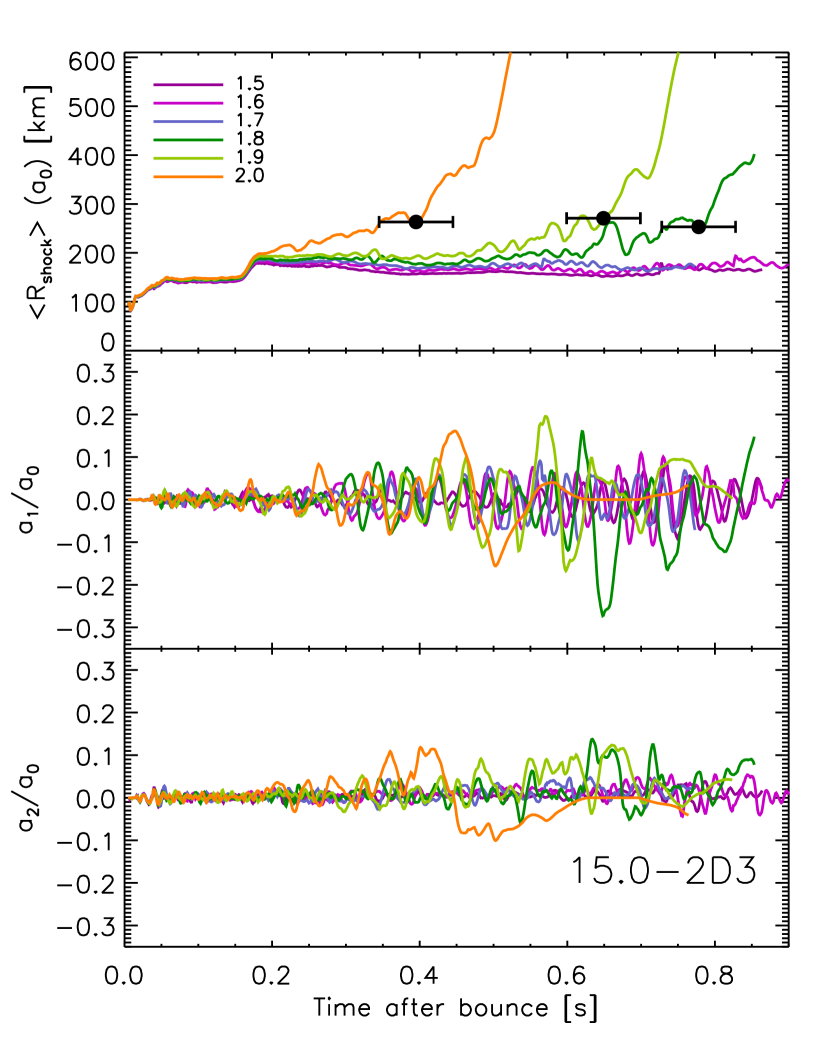
These temporal coefficients for the 15.0-2D3 sequence are plotted in Fig. 3. The average shock radius, $a_{0}$ or $\langle R_{\rm shock}\rangle$, is shown in the top panel, and a dot indicates the time of explosion, $t_{\rm exp}$ for the exploding models. Accompanying are error bars indicating an estimated uncertainty of $t_{\rm exp}$ (see §7 for the definition of $t_{\rm exp}$). The $\ell=1$ and $\ell=2$ components normalized by $a_{0}$ are shown in the middle and bottom panels. First of all, note that the range of luminosities bracketing the critical luminosity for the 2D simulations in Fig. 3 are lower than the range for 1D simulations in Fig. 2. Further comparison indicates that, unlike 1D simulations, 2D simulations show very little oscillation in $\langle R_{\rm shock}\rangle$ prior to explosion. In fact, oscillations in $\langle R_{\rm shock}\rangle$ are miniscule for non-exploding models and only reach $\sim$10% around $t_{\rm exp}$ for exploding simulations.

Instead, SASI originated oscillations in $\ell=1$ and $\ell=2$ components dominate the non-exploding and exploding models. The amplitudes of the dipole component, $a_{1}/a_{0}$, for $L_{\nu_{e}}=1.5$ remain low at $\sim$2.5%, from bounce until 500 ms. Around 500 ms, the amplitude grows to $\sim$10%. On the other hand, models with $L_{\nu_{e}}=1.6$-1.9 show a steady rise to $\sim$10% from bounce. Exploding models, for which $L_{\nu_{e}}=1.8$, 1.9, and 2.0, show an abrupt increase in amplitude to $\sim$20%. For non-exploding models, $a_{1}/a_{0}$ saturates at $\sim$10%, and for $L_{\nu_{e}}=1.5$ and 1.6 it decreases to $\sim$5%. At early times, simulations with $L_{\nu_{e}}=1.5$ and $L_{\nu_{e}}=2.0$ show the lowest and highest SASI amplitudes, respectively, and are easily distinguished from the other simulations. While this would suggest a correlation in SASI amplitude with $L_{\nu_{e}}$, the other models do not show a similar monotonic trend. Rather their amplitudes occupy the region between $L_{\nu_{e}}=1.5$ and $L_{\nu_{e}}=2.0$ but show no discernible trend with luminosity. The quadrupole term, $a_{2}/a_{0}$, is generally below $\sim$5% during non-exploding phases. For times just before explosion and afterward, $a_{2}/a_{0}$ can reach $\sim$10%.

Two important results are apparent in Figs. 2 and 3. A critical luminosity separates exploding and non-exploding models in time-dependent 1D and 2D simulations, and the critical luminosity for 2D simulations is $\sim$70% of the critical luminosity for 1D models. More evidence will be presented in §8 that the critical luminosity depends upon $\dot{M}$. For 1D simulations, we observe pulsations near the critical luminosity, but in 2D simulations, radial oscillations are all but absent. Instead, non-radial SASI oscillations dominate.

5. Effects of the Grid

The conclusions of the previous section might depend upon the grid structure used in 2D simulations. To address this concern, we investigate the dependence of these results on resolution and the range of polar angle, $\theta$, included in the simulations. Encoded in the sequence names (Table 1) are the types of grids used for 2D simulations. For calculations that encompass the full range of $\theta$ from pole to pole (180^∘) $\theta$ is divided into 200 zones, and for simulations that include only the region between a pole and the equator (90^∘) $\theta$ is divided into 100 zones. Sequences that use the 180^∘ grid have ‘2D’ in their name, and for sequences that use the 90^∘ grid, ‘Q’ is in its stead. The numbers after ‘2D’ or ‘Q’ indicate the resolution. The lowest resolution, denoted by ‘1’, extends the spherical grid from the outer edge of the butterfly mesh, 34 km, to 4000 km with 150 radial zones. The middle resolution, ‘2’, divides this same space into 300 radial zones, and the highest resolution, ‘3’, divides the radii between 34 km and 1000 km into 300 zones. For all resolutions, the space between the butterfly mesh and the outer boundaries are positioned logarithmically. These simulations do show nontrivial differences in the SASI and post-shock flow. However, the conclusions of the previous section are insensitive to changes in resolution and the range of $\theta$ simulated.

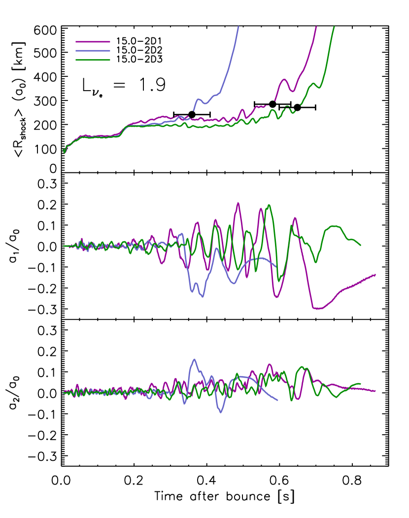
For these three resolutions, Fig. 4 shows $\langle R_{\rm shock}\rangle$, $a_{1}/a_{0}$, and $a_{2}/a_{0}$ vs. time for a single luminosity, $L_{\nu_{e}}=1.9$, and the 15-M_☉ progenitor model. Their general evolution is similar to what was discussed in §4 and shown in Fig. 3. However, there are some nontrivial differences.

After the Si/O interface is accreted, $\langle R_{\rm shock}\rangle$ of the lowest resolution model (15.0-2D1) secularly creeps out to $\sim$220 km over 100 ms. Then, outward progression stalls again, and the model doesn’t explode until 581 ms after bounce. Both the 15.0-2D2 and 15.0-2D3 models momentarily stall at $\sim$200 km, a smaller radius. 150 ms later, the average shock radius of the 15.0-2D2 model reaches $\sim$220 km on its way to explosion. At an even later time, 550 ms, the shock radius of the 15.0-2D3 model reaches $\sim$220 km. By this measure, the trend with resolution is monotonic. However, this does not translate to monotonicity in explosion time with resolution. From the lowest resolution (15.0-2D1) to the highest resolution (15.0-2D3), the explosion times are 581, 359, and 649 ms. Yet, considering another luminosity, $L_{\nu_{e}}=2.0$ (see Table 2) does present a monotonic trend toward later explosion times with higher resolution: from the lowest to the highest resolution, $t_{\rm exp}=325$, 364, and 395 ms. From this, one might conclude that higher-resolution grids forestall explosion, yet only the highest resolution shows an explosion for $L_{\nu_{e}}=1.8$.

The $\ell=1$ and $\ell=2$ (the middle and bottom panels of Fig. 4) spherical harmonic coefficients, like the monopole term, show some differences with resolution, but present very few clear trends. Any trends that do appear are subtle. In the earliest phase, before accretion of the Si/O interface, the highest resolution simulations exhibit the greatest amplitude, though all three resolutions have amplitudes in the $\ell=1$ coefficient that are less than 5%. At the same time, the $\ell=2$ component is comparable for all three resolutions. After accretion of the Si/O interface, the nonradial components begin to rise for all three resolutions. From $\sim$200 to $\sim$325 ms, the 15.0-2D1 model shows the greatest increase in both nonradial components, while for 15.0-2D2 and 15.0-2D3 they are comparable in growth. At $\sim$325 ms, the 15.0-2D2 model shows a significant increase in the nonradial components that coincides with explosion. The nonradial components for the other two simulations continue a secular increase in amplitude until their explosions at later times. All the while, the lowest resolution run consistently maintains a slightly larger amplitude in the $\ell=1$ component, but the $\ell=2$ components are quite similar. Generally, before accretion of the Si/O interface, oscillation amplitudes for $a_{1}$ are mildly correlated with resolution, and afterward it is mildly anti-correlated with resolution.

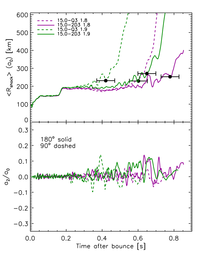
Figure 5 compares 180^∘ (15.0-2D3, solid) and 90^∘ (15.0-Q3, dashed) simulations. $\langle R_{\rm shock}\rangle$ and $a_{2}/a_{0}$ vs. time are plotted for two electron-neutrino luminosities $L_{\nu_{e}}=1.8$ (purple curves) and $L_{\nu_{e}}=1.9$ (green curves). Once again dots in the top panel mark $t_{\rm exp}$; interestingly, the 90^∘ simulations consistently explode before the 180^∘ simulations. Other than for times near $\sim$300 to $\sim$400 ms, all models show similar evolution in the amplitude of $a_{2}/a_{0}$. The one exception appears around $\sim$300 to $\sim$400 ms, when the 90^∘, $L_{\nu_{e}}=1.9$ model starts exploding and shows the largest amplitude. Even though the 90^∘ simulations explode earlier than the 180^∘ simulations, the critical luminosities for the 180^∘ and 90^∘ simulations are very similar (see Table 2 and §8).

Using a “ray-by-ray” neutrino transport algorithm, Buras et al. (2006a) performed simulations of the 11.2-M_☉ progenitor that teetered on the verge of explosion for a 90^∘ calculation, but exploded using 180^∘. They reported no explosion with a 90^∘ simulation but, with all else being equal, obtained an explosion with a 180^∘ simulation. Differences between our simulations and theirs include neutrino transport, EOS, and hydrodynamic solver. While any of these could account for the apparent discrepancy, we emphasize the difference in the 90^∘ grids. The 90^∘ simulations of Buras et al. (2006a) included a wedge that extends plus and minus 45^∘ of the equator and suppressed $\ell=1$ and $\ell=2$ modes, the two prominent modes of the SASI. Our 90^∘ simulations range from the pole to the equator and inhibit only the $\ell=1$ mode. Regardless, Buras et al. (2006a) noted that their 90^∘ simulation was close to explosion and that extending the grid to 180^∘ simply tipped the scales toward explosion. Using the same hydrodynamics and neutrino transport as Buras et al. (2006a), but a 90^∘ grid that goes from the pole to the equator, Marek (2007) found that 90^∘ simulations explode insignificantly earlier than 180^∘ simulations. In either case, these results are consistent with our finding that the critical luminosity for simulations using 90^∘ and 180^∘ are very similar.

Resolution and the angular size of the grid non-trivially affect the shock position and morphology in 2D simulations. For one, the lowest resolution simulations consistently maintain a slightly larger amplitude in the $\ell=1$ component. At early times, the lowest resolution simulations reach $\sim$220 km before higher resolution simulations. This does not lead to a monotonic correlation in explosion times, though. In changing the angular size of the grid, the 90^∘ simulations consistently explode at earlier times compared to the 180^∘ simulations. Despite differences that result from grid changes, the conclusions of the previous section do not change. Specifically, the critical luminosity for the 90^∘ and 180^∘ simulations are very similar.

6. Heating and Advection Timescales

Measures that are related to the critical $L_{\nu_{e}}$ and $\dot{M}$ condition (Burrows & Goshy, 1993) are the timescale for matter to traverse the gain region, the advection timescale, $\tau_{\rm adv}$, and the heating timescale of the matter in the gain region, $\tau_{q}$. Thompson (2000) argued that 1D core-collapse simulations do not explode because $\tau_{q}$ is longer than $\tau_{\rm adv}$. In other words, core-collapse simulations fail because $\tau_{\rm adv}/\tau_{q}<1$. He defined, $\tau_{q}\sim aT^{4}/\dot{Q}$, and the advection time as the flow time across a scale height. Janka (2001) explored similar integral concepts, and proposed conditions for explosion that are akin to

$$\tau_{\rm adv}/\tau_{q}>1\,,$$ (11)

the opposite of the Thompson (2000) failure condition. Thompson et al. (2005) applied this condition to 1D core-collapse simulations and demonstrated that this ratio does indeed help to distinguish non-exploding models from exploding models. They defined the advection timescale as $H/v_{r}$, where H is the pressure scale height, and the heating timescale as $(P/\rho)/\dot{q}$, where $\dot{q}$ is the local net heating rate. Since, others have explored $\tau_{\rm adv}$ and $\tau_{q}$ as a condition for explosion in 2D simulations (Buras et al., 2006b; Scheck et al., 2008). While $\tau_{\rm adv}/\tau_{q}>1$ is to some extent useful in identifying explosions, our results suggest that it is only useful as a rough diagnostic.

We define the heating time as a characteristic time for neutrinos to change the thermal energy of the matter in the gain region, where heating dominates cooling,

$$\tau_{q}=\frac{\int_{\rm gain}(\varepsilon-\varepsilon_{0})dm}{\dot{Q}}\,,$$ (12)

where $\varepsilon_{0}$ is the zero point energy for the EOS and

$$\dot{Q}=\int_{\rm gain}(\mathcal{H}-\mathcal{C})dm\,$$ (13)

is the net heating rate and is integrated over the gain region. While Scheck et al. (2008) and Buras et al. (2006a) include $1/2v^{2}+\Phi$ in the integrand of eq. (12), we suggest, like Thompson (2000) and Thompson et al. (2005), that comparing the heating rate to the thermal energy eq. (12) is a more natural definition of a heating timescale. To be clear though, these differences in definition alter the absolute scale, but not the general trends.

For spherically symmetric flow, the advection timescale is

$$\tau_{\rm adv}=\int_{\rm gain}\frac{dr}{v_{r}}\,$$ (14)

where the the integral is integrated from the shock position to the gain radius. For 2D simulations, many incarnations of eq. (14) have appeared in the literature. Scheck et al. (2008) use a solid-angle averaged version of eq. (14) for $\tau_{\rm adv}$. Buras et al. (2006a) use eq. (14) for the advection timescale in 1D, but for 2D simulations they redefine this timescale as the time for a mass shell to traverse the gain region. We’ve explored three measures of the advection timescale. The first replaces the denominator in eq. (14) with the solid-angle averaged velocity, $\langle v_{r}\rangle=(\int{v_{r}d\Omega})/4\pi$. For the second, if one assumes steady-state flow, then $\tau_{m}=M_{\rm gain}/\dot{M}$ is a useful measure of the accretion timescale, where $M_{\rm gain}$ is the mass in the gain region and $\dot{M}$ is the mass flux in or out of the gain region. For simplicity, we use $\dot{M}$ just exterior to the shock. The advantage of this definition is that it is relatively straightforward to measure $M_{\rm gain}$ and $\dot{M}$ for 2D simulations. Prior to explosion, these two definitions give similar results, but as the model explodes, the assumption of steady-state accretion is violated and $\tau_{m}$ begins to underestimate $\tau_{\rm adv}$. Neither of these definitions, however, fully capture the complex multi-dimensional nature of the post-shock flow.

We define a new timescale that better captures the multi-dimensional nature of the post-shock flow. Post-processing the simulation data, we integrate the paths of tracer particles for 150 ms, record their trajectories, and define a residence time, $\tau_{r}$, which is the duration of each particle’s time spent in the gain region. 50,000 particles are initiated at either 400 km, a radius well outside the shock, or 150 km, the middle of the gain region. At either radius, the particles are randomly distributed in $\mu=\cos\theta$. For most situations, the particles traverse the gain region within the integration time, 150 ms, and have accreted onto the PNS. Every 10 ms, a new generation of 50,000 particles is generated, providing a time-dependent distribution of $\tau_{r}$.

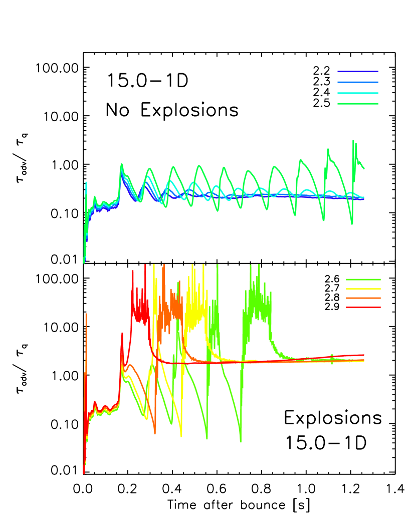
The ratio $\tau_{\rm adv}/\tau_{q}$ vs. time is shown in Fig. 6 for the 15.0-1D sequence. The top panel shows the models that do not explode by 1.3 s after bounce, and the bottom panel shows those that do explode. Despite dramatic oscillations, $\tau_{\rm adv}/\tau_{\rm q}$ rarely reaches a value of one for the non-exploding models (top panel). In all non-exploding cases, except $L_{\nu_{e}}=2.5$, the oscillations in this ratio decay with a timescale commensurate with the decay times of the shock radius oscillations (Fig. 2). For exploding models (bottom panel), $\tau_{\rm adv}/\tau_{q}$ executes large excursions from $\sim$0.1 to $\sim$100. Note that $\tau_{\rm adv}/\tau_{\rm q}$ makes several excursions to values above order unity and back again. Smaller luminosities produce more excursions, with one at $L_{\nu_{e}}=2.9$ and four for $L_{\nu_{e}}=2.6$.

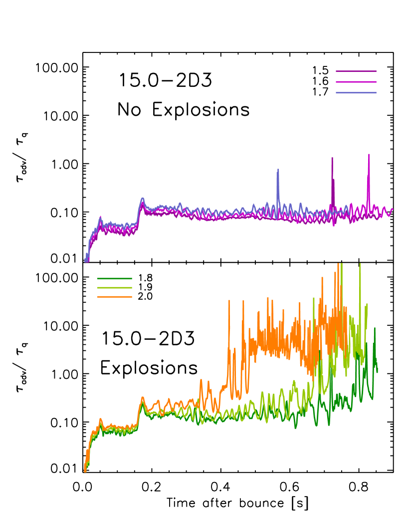
The ratio of these timescales for 2D simulations (15.0-2D3 sequence) are shown in Fig. 7. The models that don’t explode, $L_{\nu_{e}}=1.5$, 1.6, and 1.7, show relatively constant ratios for all time. On the other hand, the exploding models, $L_{\nu_{e}}=1.8$, 1.9, and 2.0, start at a low ratio ($\sim$0.1) and secularly increase to ratios of order $\sim$10. Unlike the 1D models, once this ratio reaches large values (in an average sense), it remains there for the rest of the simulation.

Generally, the condition $\tau_{\rm adv}/\tau_{q}>1$ is a useful diagnostic of explosion, but given the ambiguities in defining $\tau_{\rm adv}$ and $\tau_{q}$, its accuracy is limited. For example, 1D simulations that explode make dramatic excursions above and below this line before explosion. It might be more sensible to state that this condition should be satisfied for a finite time before explosion occurs. However, one shouldn’t expect rigor when defining a heating timescale. Note that this condition assumes a quasi-steady state, and the large amplitude oscillations in 1D complicate this assumption. Finally, $\tau_{\rm adv}/\tau_{q}$, in 2D exploding simulations, increases monotonically for $\sim$100 ms, while this ratio remains low for 2D non-exploding simulations. This distinction implies that 2D exploding models are well on their way to explosion before $\tau_{\rm adv}/\tau_{q}>1$ is satisfied. Hence, $\tau_{\rm adv}/\tau_{q}$ is a useful diagnostic for explosion, but may not be a rigorous condition for explosion.

In Fig. 8, we plot for all generations of tracer particles the mean residence times, $\langle\tau_{r}\rangle$ (top panel), and the fraction ($f_{r}$) of particles with $\tau_{r}>40$ ms (bottom panel) as a function of time for the $L_{\nu_{e}}=1.9$ model of the 15.0-2D3 sequence. The particles with $R_{\rm start}=400$ km (150 km) are shown with solid (dashed) lines. Both $\langle\tau_{r}\rangle$ and $f_{r}$ show that the particles with $R_{\rm start}=400$ km and 150 km track two fundamentally different flows. Generally, the particles with $R_{\rm start}=150$ km have longer average residence times and more particles with $\tau_{r}>40$ ms than the generation of particles with $R_{\rm start}=400$ km, which suggests that most of the mass that accretes through the shock quickly finds its way to the PNS through narrow, low entropy plumes. Despite the quick accretion of new matter, the long $\tau_{r}$ of particles with $R_{\rm start}=150$ km indicate that a significant amount of mass in the gain region does linger, resulting in more heating and higher entropies.

To verify this, we compute the total amount of mass with high entropies and compare this to the total mass in the gain region. To define high entropies, we choose a minimum entropy of 14 k_B/baryon, which corresponds to the maximum entropy for the 1D simulation of the same neutrino luminosity (see Fig. 13) and gives a rough boundary between the regions with short (low entropy) and long (high entropy) residence times. The ratio of mass with high entropy to the total mass in the gain region grows from 0% to 70% between 0.2 s and 0.5 s after bounce. For the rest of the simulation the ratio remains at this level. Therefore, even though most of the accreted mass advects quickly through the gain region via the down-flowing plumes, a significant fraction of the mass in the gain region is better characterized with long residence times and high entropies.

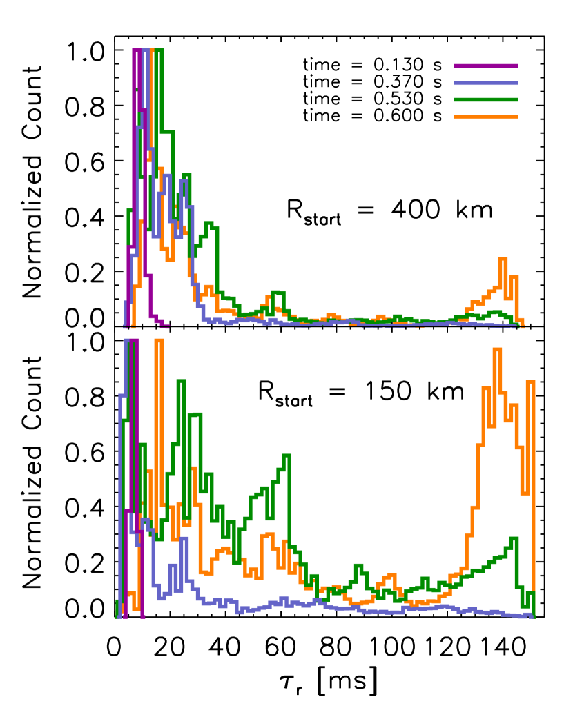
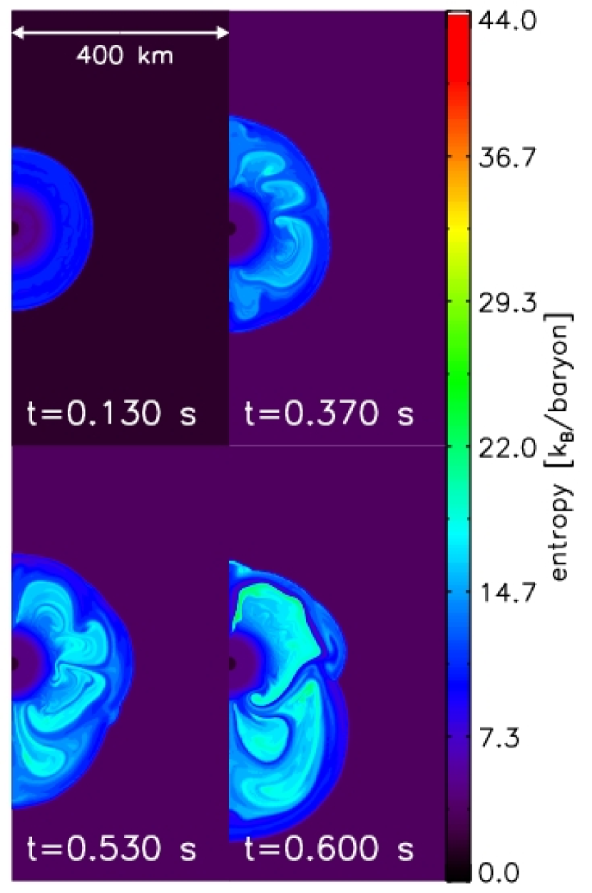
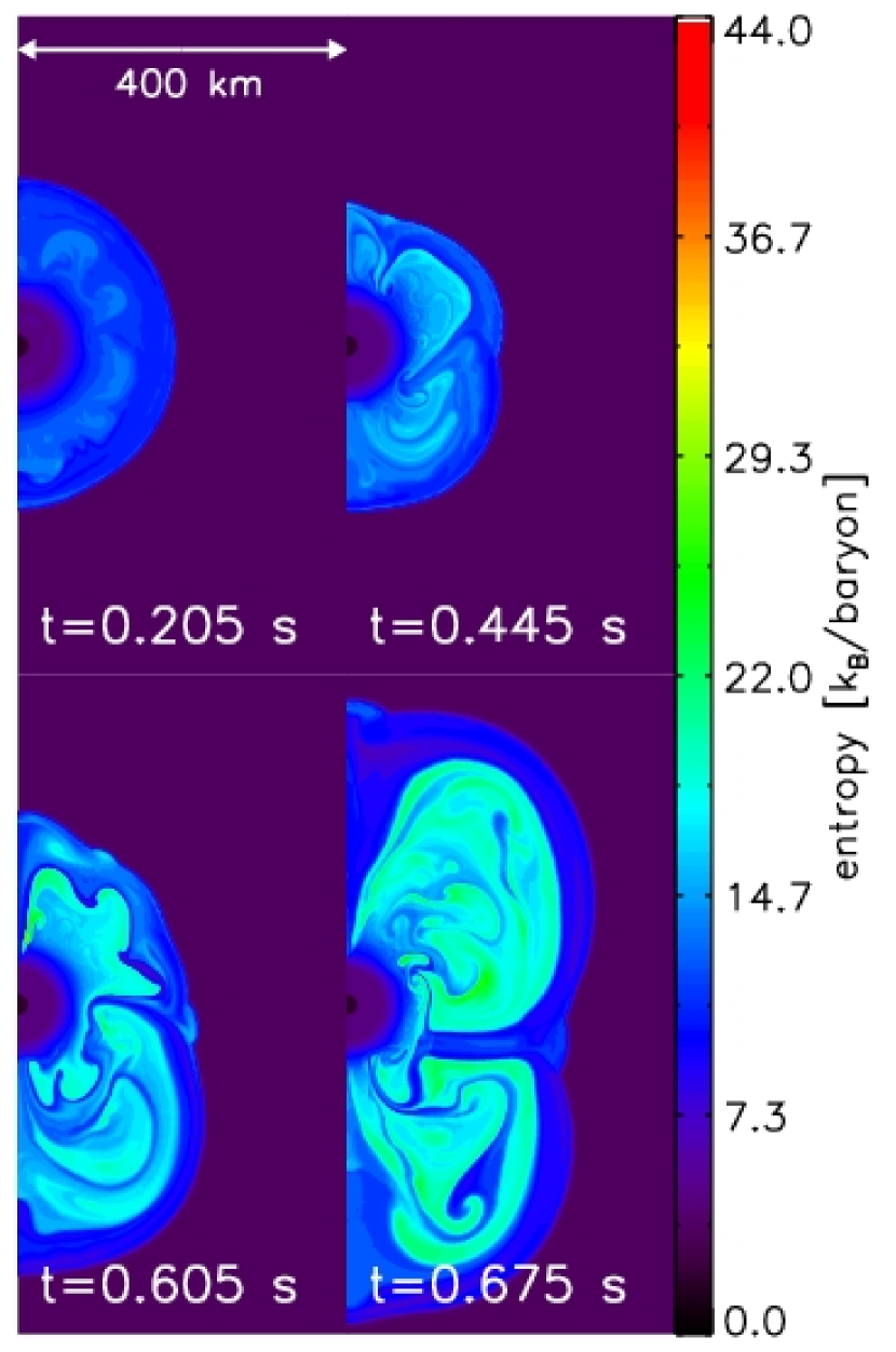
In addition, $\langle\tau_{r}\rangle$ and $f_{r}$ show four distinct phases, with each successive phase having longer $\langle\tau_{r}\rangle$ and higher $f_{r}$. Distributions of $\tau_{r}$ that represent these four phases are shown in Fig. 9, and spatial colormaps of entropy are shown in Figs. 10, 11, and 12 that correspond to the beginning (Fig. 10), middle (Fig. 11), and end (Fig. 12) of each generation’s integration time of 150 ms. The top panel of Fig. 9 shows the distribution for four generations with $R_{\rm start}=400$ km and at $t=0.130$, 0.370, 0.530, and 0.6 s after bounce. The bottom panel shows similar residence-time distributions for generations with $R_{\rm start}=150$ km.

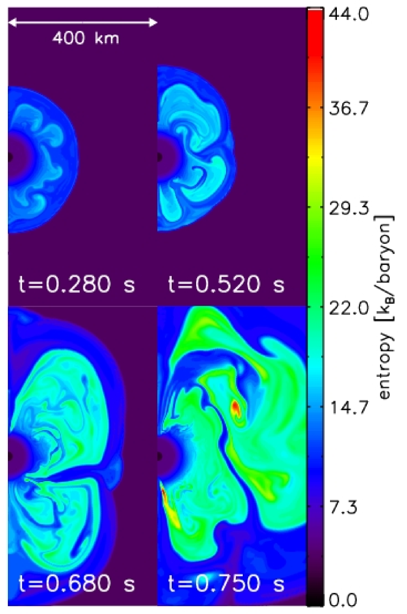
The entropy maps in the top-left panels of Figs. 10, 11, and 12 show that there is very little convection or SASI for the first phase ($t=0.130$ s), and the distributions of $\tau_{r}$ (Fig. 9) show that all particles traverse the gain region quickly, within $\sim$9 ms. At $\sim$150 ms, when the Si/O interface is accreted, both $\langle\tau_{r}\rangle$ and $f_{r}$ show a dramatic increase. The mean residence time increases from $\sim$10 ms to $\sim$40 ms for $R_{\rm start}=400$ and 150 km, and $f_{r}$ increases from 0% to 35% for $R_{\rm start}=400$ km and $\sim$50% for $R_{\rm start}=150$ km. The second phase, from $\sim$200 ms to $\sim$450 ms, corresponds to the growth and nonlinear saturation of the SASI (top-right panels of Fig. 10-12). During this phase ($t=0.370$ s in Fig. 9), $\langle\tau_{r}\rangle$ for $R_{\rm start}=400$ km (150 km) is $\sim$22 ($\sim$32), and $f_{r}$ is $\sim$10% ($\sim$30%). The third phase, from $\sim$0.45 to $\sim$0.6 s, shows a rise in both $\langle\tau_{r}\rangle$ and $f_{r}$. The distributions in Fig. 9 that represent this phase, $t=0.530$ s, have mean residence times of $\sim$50 ms ($\sim$30 ms) for $R_{\rm start}=150$ km (400 km) and $f_{r}$ of 50% (20%). The fourth and final phase is marked by a significant increase of $\langle\tau_{\rm res}\rangle$ and $f_{\rm res}$ for $R_{\rm start}=150$ km particles and continued rise for $R_{\rm start}=400$ km. In Fig. 9, the example distribution is shown at $t=0.6$ s. For $R_{\rm start}=400$ km, $\langle\tau_{\rm res}\rangle\sim 40$ ms and $f_{\rm res}\sim 25$%, while $\langle\tau_{\rm res}\rangle\sim 90$ ms and $f_{\rm res}\sim 70$%. This phase is also characterized by a large bump of particles with very long residence times in Fig. 9, which is much larger for $R_{\rm start}=150$ km than for $R_{\rm start}=400$ km. The appearance of the bump at large $\tau_{r}$ is one of the most pronounced indicators that the star has reached an explosive situation.

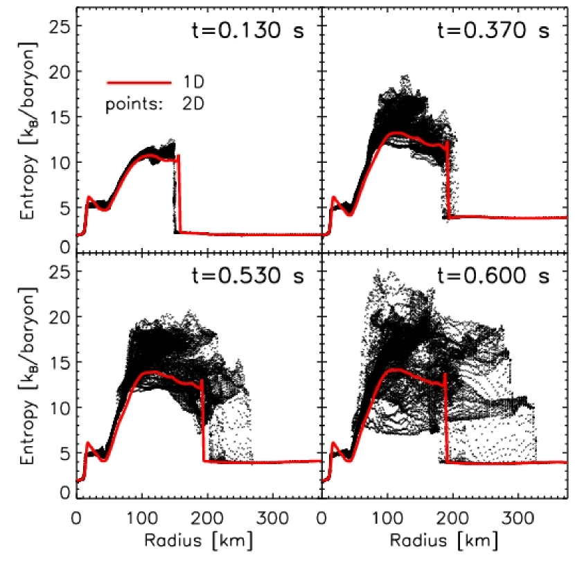
In Fig. 13, we compare 1D entropy profiles of the 15.0-1D, $L_{\nu_{e}}=1.9$ simulation (solid red lines) with the entropy distributions shown in Fig. 10. For each zone of the 2D simulation, points mark the entropy and radius from the center. Generally, both 1D and 2D profiles show the shock as an abrupt jump in entropy of the accreting matter, the gain region as indicated by the highest entropies, and the cooling region where entropy is significantly reduced as matter continues to accrete onto the PNS. Where 1D profiles show a negative entropy gradient, 2D simulations are convective. The most striking differences, though, are that when the SASI dominates the post-shock flow, $t=0.370$, 0.530, and 0.600 s, the shock is asymmetric, and the gain region has a large range of entropies, in which high entropies correspond to regions of long residence times, and low entropies correspond to plumes that funnel matter toward the PNS.

Other than passage through shocks, the entropy is determined by neutrino heating and cooling. Therefore, entropy is a good measure of the integrated history of net heating. Considering mass- and volume-weighted averages, the entropy for 2D simulations is a couple $k_{B}$/baryon (less than 10%) higher than 1D simulations. However, Fig. 13 shows that 2D simulations have regions with $\sim$30% higher entropies than 1D simulations for the same $L_{\nu_{e}}$ and $\dot{M}$. In other words, the long residence times that accompany the SASI in 2D simulations result in regions with higher integrated net heating and offer an explanation for the lower critical luminosity of 2D simulations.

7. Conditions at Explosion

As relevant indicators of the core-collapse mechanism, we investigate the net heating rate ($\dot{Q}$), heating efficiency ($\dot{Q}/L_{\nu_{e}\bar{\nu}_{e}}$), and the mass in the gain region ($M_{\rm gain}$). In general, these quantities show distinctly different evolutions for 1D and 2D simulations near their respective critical luminosities. Plots of the 1D simulations reflect the very large radial shock oscillations, while plots of the 2D simulations show relatively smooth evolution and bifurcations distinguishing explosive models from non-explosive models. Scheck et al. (2008) compared these quantities for 1D and 2D simulations with the same neutrino luminosity and found similar bifurcations in these integral measures. We show that this bifurcation is generic when we include 1D and 2D non-exploding and 2D exploding models. In Table 2, we summarize the conditions at explosion, but first we take care to define $t_{\rm exp}$, the time of explosion.

The time of explosion for 1D simulations is quite pronounced and occurs near the time when the ratio $\tau_{\rm adv}/\tau_{q}$ becomes of order unity or larger for the last time. However, for 2D simulations, all measures show a gradual trend toward explosion over 50 to 100 ms timescales. Therefore, to define $t_{\rm exp}$ we identify the last time that $\tau_{\rm adv}$ is less than 50 ms (65 ms) for 15-M_☉ (11.2-M_☉) models. This definition establishes the time of explosion after there is a clear trend toward explosion, but before post-shock material is launched outward. Acknowledging the ambiguity of such a definition, we assign an uncertainty to $t_{\rm exp}$ of $\pm 50$ ms.

Having defined $t_{\rm exp}$, we now define the conditions at explosion. For 1D simulations, $\dot{M}_{\rm exp}$ is defined at 250 km and at $t_{\rm exp}$. For 2D simulations, $\dot{M}_{\rm exp}$ is defined just exterior to the shock (at roughly 300 to 250 km) at the time of explosion. Corresponding to the uncertainty in $t_{\rm exp}$, we determine the uncertainty in $\dot{M}_{\rm exp}$. Figs. 14, 15, and 16, show a general upward trend of $\dot{Q}$, $\dot{Q}/L_{\nu\bar{\nu}_{e}}$, and $M_{\rm gain}$ around the time of explosion. The values in Table 2 are obtained by averaging $\dot{Q}$, $\dot{Q}/L_{\nu\bar{\nu}_{e}}$, and $M_{\rm gain}$ for a 50 ms range centered on $t_{\rm exp}$. We also experimented with a range of 10 and 100 ms and obtained similar results. For 1D simulations, we note the conditions at the time of explosion, but due to large nonlinear oscillations the specific values are sensitive to the definition of $t_{\rm exp}$.

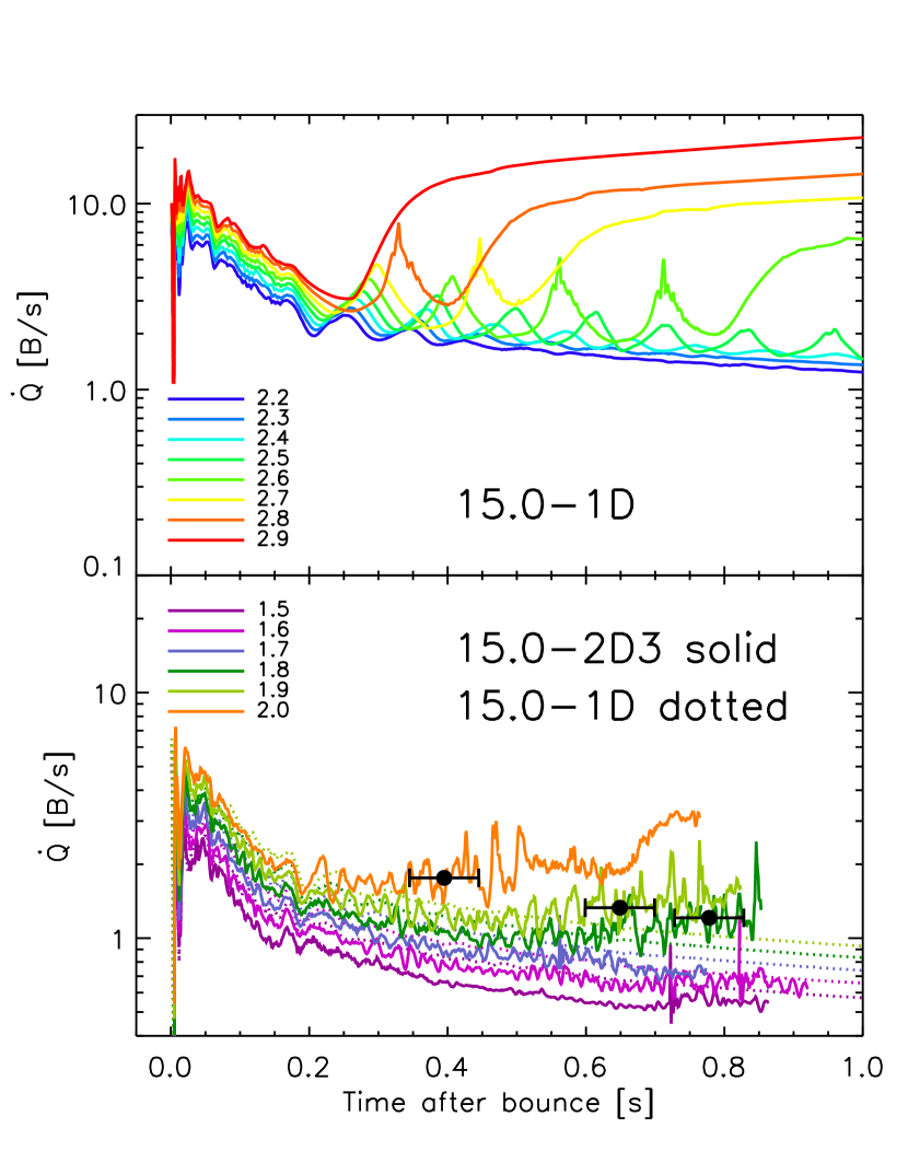
Figure 14 compares the time evolutions of the net heating rates, $\dot{Q}$, for the 15.0-1D and 15.0-2D3 sequences. While the top panel shows $\dot{Q}$ for the sequence of 1D simulations near explosion, the bottom panel shows $\dot{Q}$ for the sequence of 2D simulations (solid) near explosion. For comparison, 1D models (dotted) for the same range of $L_{\nu_{e}}$ as the 2D sequence are included. The dots show $\dot{Q}$ at the time of explosion for the 2D simulations. As expected, $\dot{Q}$ correlates with $L_{\nu_{e}}$ (Fig. 14). Consequently, the range of $\dot{Q}$ for the 1D exploding models ($\sim$1 to $\sim$11 B/s, where 1 Bethe (B) $=10^{51}$ erg) is higher than the range of $\dot{Q}$ for the 2D exploding models ($\sim$0.5 to $\sim$6 B/s). The 1D sequence in the top panel shows pronounced oscillations in $\dot{Q}$ that correspond to the oscillations in shock radius in Fig. 2. The maxima in $\dot{Q}$ coincide with the minima in the shock radius, which has been observed before for 1D simulations (Buras et al., 2006b).

The 2D sequence, on the other hand, shows no such oscillations in $\dot{Q}$. Rather, the bottom panel of Fig. 14 shows a relatively smooth evolution with time. After bounce, $\dot{Q}$ evolves secularly downward for non-exploding 1D and 2D simulations. In contrast, 50 ms to 100 ms before $t_{\rm exp}$, $\dot{Q}$ for exploding 2D simulations remains flat with time or even begins to rise slightly. In either case, there is a clear bifurcation in the evolution for exploding 2D simulations and non-exploding 1D and 2D simulations.

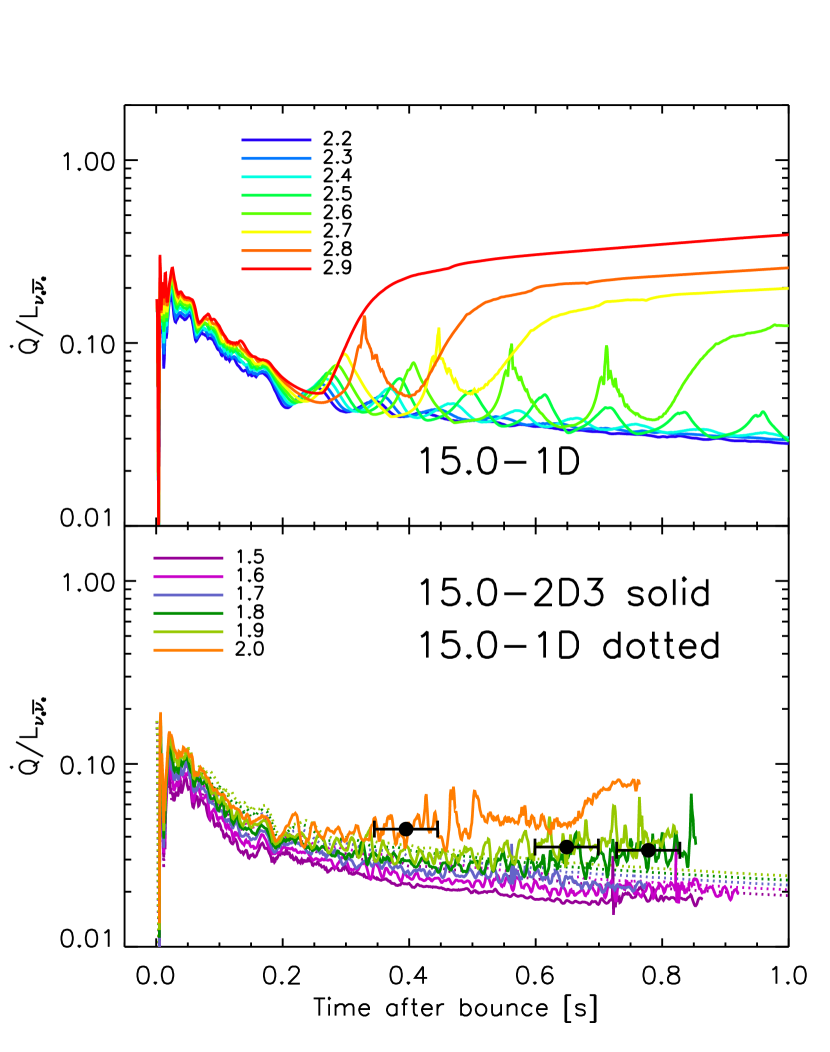
Similar to Fig. 14, in Fig. 15 we plot the heating efficiency, $\dot{Q}/L_{\nu_{e}\bar{\nu}_{e}}$. Even after dividing by $L_{\nu_{e}\bar{\nu}_{e}}$ the efficiency has a positive correlation with $L_{\nu_{e}}$. This suggests that the correlation between $\dot{Q}$ and $L_{\nu_{e}}$ is steeper than linear. The efficiencies at $t_{\rm exp}$ for the 1D sequence range from 3% to 10%, while the efficiencies of the 2D simulations at $t_{\rm exp}$ are 3.4%, 3.5%, and 4.4% for $L_{\nu_{e}}=1.8$, 1.9, and 2.0, respectively. Naturally, the trends in $\dot{Q}/L_{\nu_{e}\bar{\nu}_{e}}$ are similar to the those of $\dot{Q}$, including the bifurcation of $\dot{Q}/L_{\nu_{e}\bar{\nu}_{e}}$ for exploding and non-exploding models.

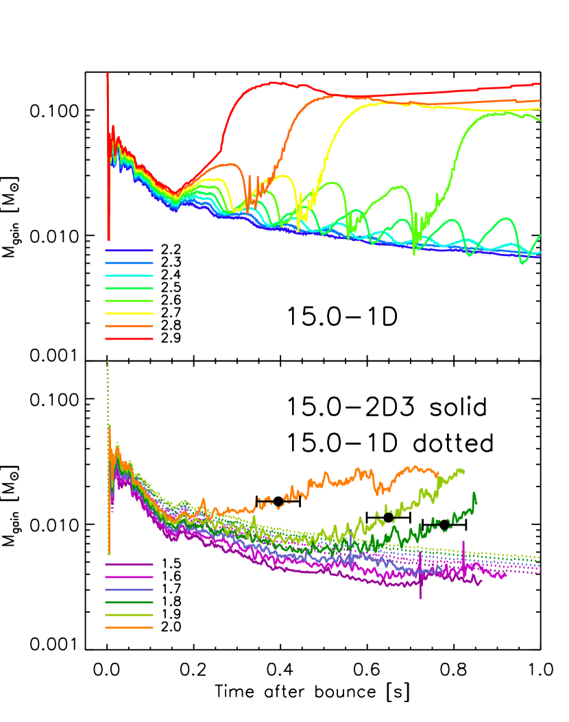
Fig. 16 shows the time evolution of $M_{\rm gain}$ for the 15.0-1D and 15.0-2D3 sequences. Once again, the oscillations in $M_{\rm gain}$ correspond to the oscillations in shock radius, but this time the minima in $M_{\rm gain}$ correspond to the minima in shock radius. In the exploding models of 15.0-2D3, there is a clear secular increase in the amount of mass in the gain region leading up to and past explosion. This is consistent with the idea that the SASI helps to increase the amount of mass in the gain region, tipping the scales toward explosive solutions. However, we note in Fig. 3 that even the non-exploding models show some $\ell=1$ oscillations, and hence, the SASI is necessary but not sufficient in increasing the mass in the gain region. At $t_{\rm exp}$, $M_{\rm gain}=$ 0.099, 0.0113, and 0.0152 M_☉ for $L_{\nu_{e}}=1.8$, 1.9, and 2.0, respectively.

We summarize the conditions at explosion in Table 2. We list for each sequence in Table 1, the electron-neutrino luminosity, $L_{\nu_{e}}$ (column 1), time of explosion, $t_{\rm exp}$ (column 2), accretion rate at the time of explosion near the shock, $\dot{M}_{\rm exp}$ (column 3), the net heating rate, $\dot{Q}$ (column 4), the heating efficiency, $\dot{Q}/L_{\nu_{e}\bar{\nu}_{e}}$ (column 5), and the mass in the gain region at the time of explosion, $M_{\rm gain}$ (column 6). The mass accretion rate at $t_{\rm exp}$ is addressed in the next section. The 11.2-1D sequence manifests a wide range of $\dot{Q}$, from 0.63 to 4.46 B/s, and the range of the corresponding heating efficiencies is similarly wide, from 2.4% to 14%. In contrast, the 15.0-1D models have much larger $\dot{Q}$ at $t_{\rm exp}$, but with a smaller range. Typically they are $\sim$3.5 B/s with one at 5.57 B/s. The heating efficiencies are similarly high, $\sim$5.9 to $\sim$10%. On the other hand, 2D simulations have lower efficiencies at explosion. All 2D models that use the 15-M_☉ progenitor have $\dot{Q}$ that lies in the range $\sim$1 to $\sim$2 B/s, and have efficiencies that range from $\sim$3 to $\sim$4%. For most models, $M_{\rm gain}$ at $t_{\rm exp}$ is $\sim$0.01 M_☉, but can be as low as 0.0073 M_☉ and as high as 0.0319 M_☉.

In Figs. 14, 15, and 16, the exploding 2D models show distinctly different values of these indicators compared to those of the non-exploding 1D and 2D simulations. $\dot{Q}$, $\dot{Q}/L_{\nu_{e}\bar{\nu}_{e}}$, and $M_{\rm gain}$ trend downward for the non-exploding models. Just before, during, and after explosion, the heating rate, heating efficiency, and gain mass increase with time for the 2D exploding models. Scheck et al. (2008) have shown a similar trend in comparing 1D and 2D models at the same neutrino luminosity, and we show that this bifurcation exists among the 2D exploding and non-exploding models as well.

8. Critical Luminosity and Mass Accretion Rate

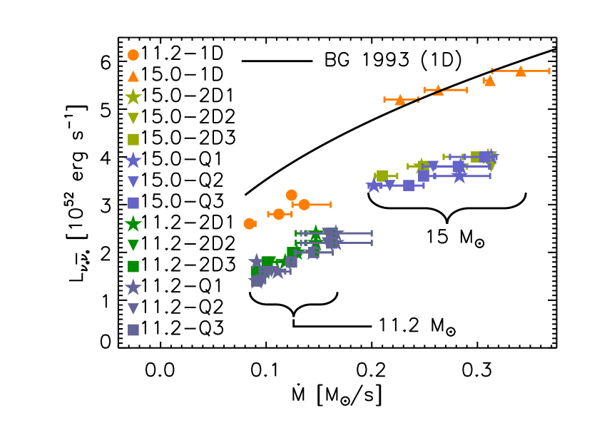
Figure 17 indicates that the concept of a critical luminosity versus accretion rate condition is relevant for time-dependent 1D and 2D simulations and quantifies the difference in critical luminosity between 1D and 2D simulations. It plots electron- plus anti-electron-neutrino luminosity, $L_{\nu_{e}\bar{\nu}_{e}}$ , vs. accretion rate, $\dot{M}$. The trajectory of each model evolves from right to left as the accretion rate decreases with time and the luminosity is held constant. For models that explode, we plot the luminosities and accretion rates at explosion. These points strongly suggest $L_{\nu_{e}\bar{\nu}_{e}}$-$\dot{M}$ curves that separate exploding from non-exploding models. Indeed, models that do not explode remain in the low luminosity and high-accretion-rate realm that is delineated by the critical curves. With error bars, we show the range of accretion rates encompassed by $t_{\rm exp}\pm 50$ ms. In general, 1D simulations are represented by orange, 2D simulations by green hues, and 2D-90^∘ runs by blue hues. The three resolutions are represented by stars (1), upside-down triangles (2), and squares (3). The fit for $L_{\nu_{e}\bar{\nu}_{e}}$ as a function of $\dot{M}$ from Burrows & Goshy (1993) is plotted (solid line). While their fit passes through the 15.0-1D points, it overpredicts the critical luminosities for the 11.2-1D runs by $\sim$15%. The critical luminosity for all 2D simulations is $\sim$70% of the critical luminosity for 1D calculations.

It is interesting that the points for the 15.0-1D sequence are consistent with the results of Burrows & Goshy (1993). However, we caution against interpreting this coincidence too literally. While we do employ very similar heating and cooling terms, it is not a priori clear how the many differences between our more realistic time-dependent models should compare to the assumptions made in Burrows & Goshy (1993) to obtain steady-state solutions.

Furthermore, we note that the slope of our results differ from the slope of the Burrows & Goshy (1993) fit and the trend is discontinuous between the 11.2 and 15 M_☉ results. The fit from Burrows & Goshy (1993) assumed a specific mass for the PNS, while our simulations have masses that naturally arise from the initial Fe-core mass and the subsequent accretion rates. Just after the Si/O interface accretes onto the PNS, the mass of the PNS, $M_{\rm PNS}$, is $\sim$1.3 M_☉ baryonic for the 11.2-M_☉ progenitor and $\sim$1.45 M_☉ baryonic for the 15-M_☉ progenitor. Afterwards, the progenitor-dependent accretion rates continue to increase the mass until explosion. Of the models from the 15.0-2D3 suite that exploded, the PNS masses at $t_{\rm exp}$ are 1.63, 1.59, and 1.52 M_☉ for $L_{\nu_{e}}=1.8$, 1.9, and 2.0. In contrast, the masses from the 11.2-2D3 suite are 1.4, 1.38, 1.35, 1.33, and 1.32 M_☉ for $L_{\nu_{e}}=0.8$, 0.9, 1.0, 1.1, and 1.2, respectively. Assuming that the explosion mechanism can be described by the transition from steady-state accretion to a neutrino-driven wind (see Burrows (1987) and Burrows & Goshy (1993), and work in preparation), we expect the critical luminosity to have a mass dependence of $L_{\nu_{e}}\propto M_{\rm PNS}^{4/5}$. Interestingly, this scaling with PNS mass resolves the slope discrepancy and the discontinuity between the 15 and 11.2-M_☉ models in Fig. 17.

Although the concept of a critical $L_{\nu_{e}}$ and $\dot{M}$ condition was derived using steady-state accretion models (Burrows & Goshy, 1993), Fig. 17 shows that the condition is appropriate for time-dependent 1D and 2D models. We find that the critical luminosity for explosion is a function of $\dot{M}$, and that it roughly follows the trend suggested by Burrows & Goshy (1993). The critical luminosity for explosions in 2D is $\sim$70% of the luminosity required for explosions in 1D simulations. While there are differences between the 90^∘ and 180^∘ simulations and between simulations with different resolutions, they roughly show the same reduction in critical luminosity when we go to 2D.

9. Conclusions

Since Burrows & Goshy (1993) published the critical luminosity condition for explosions by the neutrino mechanism, the relevance of this condition for 1D and 2D time-dependent simulations has remained unresolved. Furthermore, recent simulations have hinted that 2D simulations teeter on the verge of explosion, when 1D simulations completely fail. One wonders if the concept of a critical condition in 2D simulations can quantitatively explain the trend toward successful explosions by the neutrino mechanism.

With 95 simulations that parameterize $L_{\nu_{e}}$, $\dot{M}$, resolution, and dimensionality, we investigate the criteria for neutrino-driven explosions. The results of which indicate that:

• A critical luminosity and accretion rate condition is observed in time-dependent 1D simulations. Burrows & Goshy (1993) used the success and failure of obtaining steady-state accretion solutions to suggest a critical luminosity and mass accretion rate condition for explosions. Others have found a critical neutrino luminosity condition for explosion in time-dependent 1D simulations (Ohnishi et al., 2006; Buras et al., 2006b). We note that a critical luminosity is applicable for time-dependent 1D simulations and that it is dependent upon $\dot{M}$, as suggested by Burrows & Goshy (1993).

• Radial oscillations are characteristic of the transition between 1D accretion (non-exploding) and exploding simulations. Our results add to a growing body of literature that obtain radial oscillations near the critical luminosity (Mayle, 1985; Ohnishi et al., 2006; Buras et al., 2006b).

• A critical $L_{\nu_{e}}$ and $\dot{M}$ condition distinguishes accretion and exploding models of time-dependent 2D simulations.

• Unlike 1D simulations, radial oscillations are not prominent near the critical luminosity of 2D simulations. Rather non-radial SASI oscillations characterize 2D simulations, even for non-exploding models.

• We suggest that $\tau_{\rm adv}/\tau_{q}$ is a useful diagnostic for explosion, but may not be a rigorous condition for explosion. Specifically, we found that some 1D models strongly satisfied this condition several times before explosion, and 2D models that exploded exhibited trends toward explosion well before this condition was met.

• Several integral quantities such as heating rate, heating efficiency, and mass in the gain region grow with time in 1D and 2D exploding models, while they decline in 1D and 2D non-exploding models. Scheck et al. (2008) compared these quantities for 1D and 2D simulations with the same neutrino luminosity and found declining evolutions in the 1D non-exploding model and increasing trends in the 2D exploding model. We find similar trends. From these results, one might suggest that the SASI leads to increases in gain region mass and net heating rate, which in turn leads to explosion. However, 2D simulations that do not explode despite having pronounced SASI oscillations show declining curves. Furthermore, 1D exploding models also show increases in heating rate and gain region mass at explosion. Therefore, we conclude that the rise in these quantities near explosion are not a unique result of the SASI. Instead, the upward evolution is correlated with explosion, whether it be in 1D or 2D simulations. This, combined with the fact that the integral measures change from declining to increasing evolution near explosion, suggests that the upward trends are a consequence of explosion rather than a cause of explosion.

• We suggest an improved measure of the residence time of matter in the gain region, $\tau_{r}$, that better elucidates the conditions leading to explosions. While $\tau_{\rm adv}$ is a convenient measure of the timescale that a parcel of mass is exposed to net heating, we find $\tau_{r}$ a more informative measure for diagnosing the conditions and criteria leading to and during explosion in 2D simulations. For example, by following the trajectories of particles that start outside and within the gain region, we note that much of the mass that accretes through the shock receives very little heating as it quickly advects onto the inner core. On the other hand, there is a significant amount of mass within the gain region that has long residence times and receives a great deal of neutrino heating. It is this latter material that experiences longer and longer residence times and prolonged heating that likely reverses accretion into explosion.

• Resolution does affect the SASI and the post-shock flow in 2D simulations, but hardly alters the critical luminosity and accretion rate condition. It noticeably alters the explosion time, but the correspondence between $t_{\rm exp}$ and resolution is not monotonic, nor is it easy to disentangle the trends. However, the 2D critical luminosity vs. $\dot{M}$ curve is little affected by resolution.

• The 90^∘ simulations explode earlier than the 180^∘ counterpart, but again the critical luminosity condition is hardly affected. We contrast this with the results of Buras et al. (2006a) who found an explosion for a 180^∘ simulation, while a 90^∘ simulation did not explode. However, their 90^∘ simulation is $\pm 45^{o}$ of the equator and suppresses $\ell=1$ and $\ell=2$ nonradial flow, the dominant components of the SASI. We simulated the region from the pole to the equator, which suppresses $\ell=1$ but allows $\ell=2$. In agreement with our results, Marek (2007) found earlier explosions for 90^∘ compared to 180^∘ simulations using the same hydrodynamics and neutrino transport as Buras et al. (2006a) but a 90^∘ grid similar to ours. In any case, Buras et al. (2006a) speculated that their 90^∘ simulation was close to explosion and not very different than the 180^∘ simulation, and we show that the critical luminosity for simulations using 90^∘ and 180^∘ are very similar.

• The critical luminosity for explosions in 2D simulations is $\sim$70% of the luminosity required for explosions in 1D simulations. Irrespective of resolution or the angular size of the simulation, this conclusion holds.

By employing local heating and cooling algorithms, we avoid expensive neutrino transport, but we also sacrifice accuracy. In our simulations, heating and cooling by neutrinos are decoupled from one another, which is not consistent with neutrino transport calculations. In addition, simulations using MGFLD (Dessart et al., 2006) and “ray-by-ray” Boltzmann transport (Marek & Janka, 2007) have neutrino luminosities that decrease by $\sim$50% from 100 ms to 300 ms past bounce. Our constant $L_{\nu_{e}}$ certainly does not reflect this evolution in neutrino luminosities. Furthermore, a large fraction of $L_{\nu_{e}}$ is derived from accretion at early times (Scheck et al., 2006). In our simulations, $L_{\nu_{e}}$ is completely decoupled from such effects, and, hence, we ignore any feedback due to this coupling. While our assumptions compromise the accuracy of the results, they enable the parameter study that we present, and we suspect that the general conclusions and trends regarding the critical luminosity condition are still relevant for simulations including detailed transport.

Marek & Janka (2007) suggest that using a softer EOS in conjunction with general relativistic gravity leads to more compact PNSs and more favorable conditions for explosion; we include neither effect. The soft EOS that accompanies explosion has an incompressibility of nuclear matter, $K$, of 180 MeV, while the stiffer EOS, which does not explode, has $K=263$ MeV. While this suggests an interesting dependence of explosion on the EOS, we note that laboratory experiments indicate that $K=240\pm 20$ MeV (Shlomo et al., 2006; Lattimer & Prakash, 2007), a value that is more consistent with the non-explosive model. Regardless, with a compact PNS, the post-shock flow is positioned deeper in the potential, making it harder to explode. All else being equal, this should increase the critical luminosity. However, Marek & Janka (2007) argue that the more compact PNS is hotter, emitting more energetic neutrinos (though they are gravitationally redshifted) and at a higher luminosity, which might compensate for the higher critical luminosity. Because we parameterize the luminosity and temperature in this study, these effects are not addressed here and must await a more consistent treatment.

Of the conclusions listed above, the most striking is that time-dependent 1D and 2D simulations show a critical neutrino luminosity and accretion rate condition for successful explosions. Equally significant is that the critical luminosity for 2D simulations is $\sim$70% of the critical luminosity for 1D simulations. This quantitatively supports suspicions that multi-dimensional effects increase the likelihood of successful explosions by the neutrino mechanism. While none have explicitly explored these results, the simulations of the past decade are consistent with this conclusion, while also being intuitive and concise. In this sense, these results are expected and reassuring. Remarkably, this global condition for successful explosions, which was informed by 1D steady-state solutions, survives despite the complexities of time-dependent multi-dimensional simulations.

For all permutations of the core-collapse mechanism considered in this paper, oscillations are ubiquitous during the transition from accretion to explosion. Interestingly, the character of these oscillations for 1D and 2D simulations is quite different, and leads to distinctly different critical luminosities. Specifically, we suggest that the extra degree of freedom in 2D simulations offers an easier route to explosion via the SASI. This suggests that for other than the lightest progenitors, the core-collapse mechanism is inherently multi-dimensional, and an accurate theory for the core-collapse mechanism must be developed in the context of the multi-dimensional Universe.

Our results show that the critical luminosity for 2D simulations is lower than the critical luminosity in 1D simulations, but why is this the case? The most obvious cause is that the residence time of matter in the gain region is different for 1D and 2D simulations, and the longer residence times in 2D simulations reduce the neutrino luminosity required for explosion. So, what accounts for the different residence times when the accretion rate is the same? After all, we have shown that during the steady-state accretion phase, the advection timescales determined by the flow across the gain region ($\tau_{\rm adv}$, as calculated by eq. (14)) and by $\tau_{m}=M_{\rm gain}/\dot{M}$ are similar. Put another way, the solid-angle, average, radial velocity at radius $r$ is

$$v_{r}(r)=\frac{\dot{M}(r)}{4\pi r^{2}\rho(r)}\,,$$ (15)

and if $\rho(r)$ and $\dot{M}(r)$ are the same for 1D and 2D simulations, the flow across the gain region should be similar. Yet, 2D simulations explode when 1D simulations do not. This discrepancy can be resolved by noting that the flow in the gain region is by no means spherically symmetric in 2D simulations. The plots, histograms, and entropy maps of Figs. 8-12 show that much of the material that accretes through the shock is channeled to plumes and quickly accrete onto the PNS. At the same time, there are large regions of high entropy material that have long residence times in the gain region. When the residence times within these high entropy regions reach some threshold, it seems as though sufficient heating has occurred to launch an explosion, and because relevant regions behind the shock are in sonic contact, the shock radius expands globally. Hence, the critical luminosities for 2D simulations are lower because some matter resides for longer times in the gain region for the same $\dot{M}$.

Since the concept of a critical luminosity condition applies for 1D and 2D simulations, we assume that it should also apply for 3D simulations. Increasing the dimensionality from 1D to 2D, has proven favorable for successful explosions by the neutrino mechanism. Specifically, the extra degree of freedom in 2D simulations increases the dwell time of matter in the gain region. Similarly, we suspect that differences between 2D and 3D simulations will continue the trend toward lower critical luminosities for higher dimensions. For example, convection in 2D simulations experiences a turbulent energy cascade from smaller to larger scales. In Nature and in 3D simulations, however, the turbulent energy cascade is described well by Kolmogorov theory, in which energy cascades from larger to smaller scales. If we analyze the transport of matter through the convective gain region as a diffusive problem, then the time to diffuse through the gain region would roughly scale as

$$t_{\rm diff}\sim d\left(\frac{l^{2}}{\overline{v^{2}}\tau_{\rm coll}}\right)\,,$$ (16)

where $d$ is the number of degrees of freedom, $l$ is the characteristic size, $\overline{v^{2}}$ is the mean-squared speed of the diffusing particle, and $\tau_{\rm coll}$ is the average time between collisions. The extra degree of freedom in 3D simulations alone could increase the dwell time by $\sim$50% compared to 2D simulations. In addition, we suspect that the smaller scales of 3D simulations would produce shorter $\tau_{\rm coll}$ compared to 2D simulations and, consequently, further increase the dwell times. Whether these scaling arguments bear out in realistic 3D simulations, in which advection and the SASI are key in the flow, will be determined by future 3D simulations. If they are relevant, then the increased dwell time might result in a critical luminosity in 3D simulations that is even lower than the critical luminosity in 2D simulations. In turn, this might lead to successful explosions in 3D radiation-hydrodynamic simulations.

Table 1 Model parameters.

Sequence Name	Mass (M☉)	Dimension	$N_{r}$	$R_{\rm max}$ (km)	$L_{\nu_{e}}$ ($10^{52}$ erg s-1)
15.0-1D	15.0	1D	700	4000	1.6-2.9
15.0-2D1	15.0	2D	250	4000	1.5-2.0
15.0-2D2	15.0	2D	400	4000	1.5-2.0
15.0-2D3	15.0	2D	400	1000	1.5-2.0
15.0-Q1	15.0	2D-90∘	250	4000	1.5-2.0
15.0-Q2	15.0	2D-90∘	400	4000	1.5-2.0
15.0-Q3	15.0	2D-90∘	400	1000	1.5-2.0
11.2-1D	11.2	1D	700	4000	1.0-1.8
11.2-2D1	11.2	2D	250	4000	0.7-1.2
11.2-2D2	11.2	2D	400	4000	0.7-1.2
11.2-2D3	11.2	2D	400	1000	0.7-1.2
11.2-Q1	11.2	2D-90∘	250	4000	0.7-1.2
11.2-Q2	11.2	2D-90∘	400	4000	0.7-1.2
11.2-Q3	11.2	2D-90∘	400	1000	0.7-1.2

Table 2 Conditions at the time of explosion.

$L_{\nu_{e}}$ ($10^{52}$ erg s-1)	$t_{\rm exp}$ (ms)	$\dot{M}_{\rm exp}$ (M☉/s)	$\dot{Q}$ (B/s)	$\dot{Q}/L_{\nu_{e}\bar{\nu}_{e}}$	$M_{\rm gain}$ (M☉)
11.2-1D
1.3	932	$0.084^{+0.006}_{-0.003}$	0.63	0.0244	0.0123
1.4	496	$0.112^{+0.012}_{-0.010}$	1.50	0.0535	0.0121
1.5	312	$0.136^{+0.025}_{-0.011}$	2.00	0.0668	0.0153
1.6	409	$0.124^{+0.002}_{-0.003}$	4.46	0.1393	0.0228
15.0-1D
2.6	718	$0.227^{+0.017}_{-0.015}$	3.69	0.0710	0.0105
2.7	459	$0.263^{+0.027}_{-0.013}$	3.79	0.0701	0.0129
2.8	335	$0.312^{+0.001}_{-0.006}$	5.57	0.0995	0.0177
2.9	216	$0.341^{+0.027}_{-0.027}$	3.42	0.0589	0.0319
15.0-2D1
1.9	581	$0.247^{+0.001}_{-0.001}$	1.49	0.0392	0.0123
2.0	325	$0.310^{+0.002}_{-0.001}$	1.97	0.0494	0.0167
15.0-2D2
1.9	359	$0.313^{+0.001}_{-0.023}$	1.51	0.0399	0.0120
2.0	364	$0.313^{+0.001}_{-0.027}$	1.60	0.0401	0.0133
15.0-2D3
1.8	778	$0.210^{+0.014}_{-0.007}$	1.21	0.0337	0.0099
1.9	649	$0.249^{+0.001}_{-0.015}$	1.33	0.0351	0.0113
2.0	395	$0.299^{+0.014}_{-0.031}$	1.76	0.0440	0.0152
15.0-Q1
1.7	837	$0.202^{+0.007}_{-0.005}$	0.91	0.0268	0.0074
1.8	419	$0.283^{+0.029}_{-0.024}$	1.19	0.0330	0.0098
1.9	418	$0.284^{+0.028}_{-0.024}$	1.31	0.0344	0.0109
2.0	361	$0.313^{+0.001}_{-0.025}$	1.71	0.0428	0.0152
15.0-Q2
1.7	748	$0.217^{+0.018}_{-0.009}$	0.91	0.0267	0.0073
1.8	517	$0.249^{+0.011}_{-0.002}$	1.30	0.0362	0.0119
1.9	471	$0.258^{+0.023}_{-0.010}$	1.19	0.0314	0.0100
2.0	299	$0.310^{+0.008}_{-0.001}$	1.54	0.0385	0.0126
15.0-Q3
1.7	695	$0.235^{+0.014}_{-0.018}$	1.14	0.0335	0.0096
1.8	602	$0.249^{+0.001}_{-0.001}$	1.08	0.0301	0.0089
1.9	420	$0.282^{+0.029}_{-0.024}$	1.42	0.0373	0.0122
2.0	383	$0.307^{+0.004}_{-0.033}$	1.66	0.0415	0.0135
11.2-2D1
0.7	808	$0.091^{+0.000}_{-0.001}$	0.23	0.0165	0.0050
0.8	585	$0.098^{+0.005}_{-0.002}$	0.30	0.0190	0.0055
0.9	471	$0.118^{+0.006}_{-0.013}$	0.43	0.0242	0.0068
1.0	335	$0.129^{+0.020}_{-0.005}$	0.55	0.0276	0.0086
1.1	288	$0.147^{+0.016}_{-0.019}$	0.89	0.0404	0.0131
1.2	288	$0.147^{+0.016}_{-0.019}$	0.89	0.0370	0.0131
11.2-2D2
0.7	828	$0.092^{+0.001}_{-0.002}$	0.24	0.0170	0.0054
0.8	595	$0.097^{+0.005}_{-0.002}$	0.31	0.0193	0.0053
0.9	529	$0.104^{+0.012}_{-0.005}$	0.40	0.0220	0.0070
1.0	339	$0.128^{+0.019}_{-0.004}$	0.54	0.0268	0.0077
1.1	235	$0.163^{+0.001}_{-0.014}$	0.85	0.0386	0.0115
1.2	235	$0.163^{+0.001}_{-0.014}$	0.85	0.0354	0.0115
11.2-2D3
0.8	791	$0.091^{+0.000}_{-0.001}$	0.32	0.0200	0.0057
0.9	553	$0.101^{+0.009}_{-0.004}$	0.40	0.0225	0.0059
1.0	372	$0.125^{+0.008}_{-0.001}$	0.60	0.0300	0.0087
1.1	257	$0.162^{+0.001}_{-0.025}$	0.91	0.0413	0.0122
1.2	257	$0.162^{+0.001}_{-0.025}$	0.91	0.0378	0.0122
11.2-Q1
0.7	777	$0.091^{+0.001}_{-0.001}$	0.23	0.0165	0.0048
0.8	500	$0.111^{+0.012}_{-0.009}$	0.31	0.0191	0.0060
0.9	784	$0.091^{+0.001}_{-0.001}$	0.78	0.0434	0.0133
1.0	294	$0.144^{+0.019}_{-0.017}$	0.52	0.0260	0.0076
1.1	177	$0.166^{+0.034}_{-0.004}$	0.91	0.0414	0.0124
1.2	177	$0.166^{+0.034}_{-0.004}$	0.91	0.0379	0.0124
11.2-Q2
0.7	631	$0.096^{+0.003}_{-0.002}$	0.22	0.0158	0.0040
0.8	525	$0.105^{+0.013}_{-0.006}$	0.28	0.0174	0.0056
0.9	413	$0.124^{+0.001}_{-0.004}$	0.39	0.0218	0.0071
1.0	293	$0.145^{+0.018}_{-0.017}$	0.54	0.0269	0.0075
1.1	270	$0.158^{+0.004}_{-0.025}$	0.82	0.0371	0.0107
1.2	270	$0.158^{+0.004}_{-0.025}$	0.82	0.0340	0.0107
11.2-Q3
0.7	759	$0.091^{+0.001}_{-0.001}$	0.22	0.0160	0.0047
0.8	583	$0.098^{+0.005}_{-0.003}$	0.30	0.0186	0.0056
0.9	417	$0.124^{+0.001}_{-0.005}$	0.39	0.0218	0.0065
1.0	293	$0.145^{+0.018}_{-0.017}$	0.56	0.0282	0.0083
1.1	256	$0.162^{+0.001}_{-0.024}$	0.84	0.0383	0.0125
1.2	256	$0.162^{+0.001}_{-0.024}$	0.84	0.0351	0.0125

Figure 1.— Accretion rate, $\dot{M}$, vs. postbounce time above the stalled shock (250 km). The solid and dashed lines show the time-dependent accretion rate for the 11.2- and 15.0-M_☉ models, respectively (Woosley et al., 2002; Woosley & Weaver, 1995). While the outer portions of the Fe core accrete ($t=0$-50 ms), $\dot{M}$ is as high as 10 M_☉/s and decreases to 2 M_☉/s. After the Fe core fully accretes, the accretion rates for the two models diverge. For the 11.2-M_☉ (15-M_☉) model, it takes 50 ms (100 ms) to accrete the Si-burning shell. As the Si/O interface accretes, $\dot{M}$ plummets to 0.3 M_☉/s (0.2 M_☉/s) for the 15 M_☉ (11.2 M_☉) model. Afterward, $\dot{M}$ declines slowly to 0.2 M_☉/s (0.08 M_☉/s). Together, these two models slowly sweep through a range of accretion rates from 0.3 M_☉/s to 0.08 M_☉/s, which enables a parameterization in $\dot{M}$.

Figure 2.— Shock radius, $R_{\rm shock}$, vs. postbounce time for the 1D sequences. The top panel displays the radii for 15.0-1D, and the bottom panel shows the radii for 11.2-1D. Each line is labeled by the electron-neutrino luminosity in units of $10^{52}$ ergs s^-1. Comparing models within a sequence, all models show similar behavior prior to the accretion of the Si/O interface. The accretion of the Si/O interface either initiates an explosion or excites radial oscillations in the shock radius. For the 15.0-1D sequence, the oscillation periods range from $\sim$90 ms for $L_{\nu_{e}}=2.2$ to $\sim$170 ms for $L_{\nu_{e}}=2.8$. Of the models that oscillate, the lower luminosity simulations decay in the oscillation amplitude, while higher luminosity models oscillate and explode. The timescales for decay range from $\sim$450 ms for $L_{\nu_{e}}=2.2$ to 1.0 s for $L_{\nu_{e}}=2.5$.

Figure 3.— Shock morphology vs. postbounce time for the 15.0-2D3 sequence. The top panel shows $a_{0}$ or $\langle R_{\rm shock}\rangle$, the average shock radius, and the middle and bottom panels plot the $\ell=1$ and $\ell=2$ components divided by to the average shock radius: $a_{1}/a_{0}$ and $a_{2}/a_{0}$, respectively. The filled circles in the top panel indicate $t_{\rm exp}$, the time of explosion, and the error bars show our estimate of uncertainty ($\pm 50$ ms). Unlike the 1D models (Fig. 2), the 2D simulations show very little radial oscillation near the critical luminosity, but significant nonradial oscillations. In general, $a_{1}/a_{0}$ grows from 0% to $\sim$10% for all models, and $a_{2}/a_{0}$ grows to $\sim$5%. The $a_{1}/a_{0}$ amplitudes hint at a correlation with $L_{\nu_{e}}$ (see §4 for a discussion). Near explosion the amplitude of $a_{1}/a_{0}$ can peak around $\sim$20%.

Figure 4.— The shock morphology vs. time for three different resolutions of 2D simulations (15.0-2D1, 15.0-2D2, and 15.0-2D3). The layout is similar to Fig. 3. The electron-neutrino luminosity for each is $1.9\times 10^{52}$ ergs s^-1. From lowest resolution (15.0-2D1) to the highest resolution (15.0-2D3), the explosion times are 581, 359, and 649 ms. Hence, $t_{\rm exp}$ is not monotonic with resolution. See §5 for a discussion.

Figure 5.— $\langle R_{\rm shock}\rangle$ and $a_{2}/a_{0}$ vs. time for two models of 15.0-Q3 and 15.0-2D3. This compares the differences among the 2D runs using 180^∘ (solid) and 90^∘ (dashed). $L_{\nu_{e}}=1.8$ corresponds to the purple curves and $L_{\nu_{e}}=1.9$ corresponds to the green curves. Inspection of $\langle R_{\rm shock}\rangle$ (top panel of Fig. 5) shows that the 90^∘ simulations consistently explode before the 180^∘ simulations. Other than the time near $\sim$300 to $\sim$400 ms, all models show similar evolution in the amplitude of $a_{2}/a_{0}$. The one exception appears around $\sim$300 to $\sim$400 ms, when the 90^∘, $L_{\nu_{e}}=1.9$ model explodes and shows the largest amplitude.

Figure 6.— The ratio of advection and heating timescales, $\tau_{\rm adv}/\tau_{\rm q}$, vs. postbounce time for the 15.0-1D sequence. The top panel shows the models that do not explode by 1.3 s after bounce, and the bottom panel shows those that do explode. Despite dramatic oscillations, $\tau_{\rm adv}/\tau_{\rm q}$ rarely reaches a value of above $\sim$1 for the non-exploding models (top panel). In all non-exploding cases, except $L_{\nu_{e}}=2.5$ (in units of $10^{52}$ erg s^-1), the oscillations decay (see text and the caption of Fig. 2 for the timescales). For exploding models (bottom panel), $\tau_{\rm adv}/\tau_{q}$ makes large excursions from $\sim$0.1 to $\sim$100. Larger luminosities produce more excursions, with one at $L_{\nu_{e}}=2.9$ and four at $L_{\nu_{e}}=2.9$. We conclude that $\tau_{\rm adv}/\tau_{q}>1$ is a useful diagnostic, but not a rigorous condition for explosion.

Figure 7.— Similar to Fig. 6, but we plot $\tau_{\rm adv}/\tau_{q}$ vs. postbounce time for the 15.0-2D3 sequence. The models that don’t explode, $L_{\nu_{e}}=1.5$, 1.6, and 1.7 (in units of $10^{52}$ erg s^-1) show relatively constant ratios for all times. On the other hand, the exploding models, $L_{\nu_{e}}=1.8$, 1.9, and 2.0, start at low ratios ($\sim$0.1) and increase to ratios of order $\sim$10. Unlike the 1D models, once this ratio reaches large values, it remains there for the rest of the simulation. The times of explosion are 395, 648, and 778 ms for $L_{\nu_{e}}=1.8$, 1.9, and 2.0, respectively. Notice that the ratio of timescales begin to rise before $\tau_{\rm adv}/\tau_{q}=1$, suggesting that these models are on their way to explosion before the condition $\tau_{\rm adv}/\tau_{q}>1$ is met.

Figure 8.— The mean residence time ($\langle\tau_{r}\rangle$) (top panel) and the fraction ($f_{r}$) of particles with $\tau_{r}>40$ ms (bottom panel) as a function of time for $R_{\rm start}=400$ km (solid line) and $R_{\rm start}=150$ km (dashed line). These residence times were calculated for the 15.0-2D3, $L_{\nu_{e}}=1.9$ model. 50,000 tracer particles are initiated randomly in solid angle at either $R_{\rm start}=150$ km or $R_{\rm start}=400$ km. The trajectories for these particles are integrated for 150 ms, and a new generation is initiated every 10 ms. The time on the horizontal axis corresponds to the start time for a generation. From $\sim$200 ms and beyond, particles that start in the gain region ($R_{\rm start}=150$ km) consistently show larger $\langle\tau_{r}\rangle$ and more particles with longer residence times. There are four phases in this plot that correspond to very short residence times, steady growth in the SASI, an increase in the vigor of the SASI, and the initial stages of explosion. See §6 for a discussion and Figs. 10, 11, and 12 for entropy maps.

Figure 9.— The distribution of residence times, $\tau_{r}$, for four generations of tracer particles corresponding to the four phases in Fig. 8. The times shown in the legend correspond to the starting time for each generation, and $R_{\rm start}$ indicates the starting radius for all 50,000 particles of each generation. $R_{\rm start}=400$ km is situated well outside the shock radius, and $R_{\rm start}=150$ km is approximately the middle of the gain region. The top panel shows that most of the mass that accretes through the shock traverses the gain region on relatively short timescales, $\sim$40 ms, while the bottom panel shows that in addition to rapidly accreting plumes, there are regions in the gain region in which mass has a large residence time and is subjected to prolonged heating.

Figure 10.— Colormaps of entropy ($k_{\rm B}$/baryon) for 15.0-2D3, $L_{\nu_{e}}=1.9$ and for the four phases shown in Fig. 9. Each panel is 400 km $\times$ 800 km. These snapshots of the flow correspond to the times in Fig. 9, which label each histogram by the start time of the four generations of particles shown. The four phases are: 1) there is very little convection or SASI and the particles accrete quickly ($\sim$9 ms) onto the PNS (top left), 2) the SASI undergoes a steady growth and the particles initiated at 400 km (200 km) have a mean residence time of 22 ms (32 ms) (top right), 3) the SASI is becoming quite vigorous and the residence times for both sets of particles are steadily increasing (bottom left), and 4) The SASI is very vigorous and 150 ms later (see Fig. 12) the model undergoes explosion (bottom right).

Figure 11.— The same as Fig. 10, except the flow is shown 75 ms after the start of each generation of particles, which is the midpoint of particle tracking. Low entropy plumes that quickly transport newly-accreted material to the PNS are quite pronounced in the bottom-right panel.

Figure 12.— The same as Fig. 10, except the flow is shown 150 ms after the start of each generation of particles, which is the end of particle tracking. Note that the simulation is exploding in the bottom-right panel.

Figure 13.— Entropy vs. radius for the times shown in Fig. 10. Solid red lines are entropy profiles for the 15.0-1D, $L_{\nu_{e}}=1.9$ simulation, and points show the entropy and radius for each zone of the 15.0-2D3, $L_{\nu_{e}}=1.9$ model. These entropy profiles are coeval with the residence time distributions in Fig. 9 and the entropy maps in Fig. 10. Features of the entropy profiles highlight the shock ($\sim$150 km for $t=0.130$ s and $\sim$200 km for all other times), the gain region, ($\sim$100 km to $\sim$ 200 km), and the cooling region ($\sim$50 km to $\sim$100 km). 1D profiles show a negative entropy gradient in the gain region that results in convection in 2D simulations. When the SASI dominates the post-shock flow, $t=0.370$, 0.530, and 0.600 s, the shock is distinctly aspherical, and a large range of entropies characterize the gain region. Low entropies correspond to plumes that funnel matter onto the PNS, while high entropies correspond to regions of long residence times and more integrated net heating. This is the likely cause for 2D simulations having lower critical luminosities than 1D simulations.

Figure 14.— Time evolution of the net heating rate, $\dot{Q}$, for the 15.0-1D and 15.0-2D3 sequences. The top panel plots $\dot{Q}$ for the 1D sequence only for the range of $L_{\nu_{e}}$ near the 1D critical luminosity. The bottom panel highlights the range of $L_{\nu_{e}}$ near the critical luminosity of the 2D sequence, and plots both 1D and 2D simulations. The dots show the $\dot{Q}$ at the time of explosion for the 2D simulations. $\dot{Q}$ shows pronounced oscillations for the 1D simulations near explosion (top panel), with the peaks corresponding to dips in shock radius in Fig. 2. For non-exploding 1D and 2D simulations $\dot{Q}$ evolves downward. Exploding 2D simulations, however, have $\dot{Q}$ that tends toward flat or upward evolutions.

Figure 15.— Similar to Fig. 14, but here we plot the heating efficiency, $\dot{Q}/L_{\nu_{e}\bar{\nu}_{e}}$, vs. postbounce time. The efficiencies at $t_{\rm exp}$ for the 1D sequence near the critical luminosity range from 3% to 10%, while the efficiencies of the 2D simulations at $t_{\rm exp}$ are 3.4%, 3.5%, and 4.4% for $L_{\nu_{e}}=1.8$, 1.9, and 2.0, respectively. For non-exploding 1D and 2D simulations $\dot{Q}/L_{\nu_{e}\bar{\nu}_{e}}$ evolves downward. Exploding 2D simulations, however, have efficiencies that tend to stay flat or increase.

Figure 16.— Similar to Fig. 14, but here we plot the mass in the gain region, $M_{gain}$, vs. postbounce time. The oscillations of $M_{\rm gain}$ in the 1D models (top panel) correspond to the oscillations in shock radius. The minima in $M_{\rm gain}$ correspond to the minima in shock radius. In the exploding models of 15.0-2D3, there is a secular increase in the amount of mass in the gain region leading up to and past explosion that is distinct from the non-exploding 1D and 2D models.

Figure 17.— The electron- and anti-electron-neutrino luminosity, $L_{\nu_{e}\bar{\nu}_{e}}$ , vs. mass accretion rate, $\dot{M}$, of explosion. The accretion rate is defined just exterior to the shock at $t_{\rm exp}$. Because the time of explosion is difficult to define, we also show the range of accretion rates 50 ms before and after $t_{\rm exp}$ as error bars. In general, 1D simulations are represented by orange, 2D simulations by green hues, and 2D-90^∘ runs by blue hues. The points that lie in the $\dot{M}$ range from $\sim$0.8 to $\sim$1.7 M_☉/s correspond to simulations using the 11.2-M_☉ progenitor, and the points in the range from $\sim$0.2 to $\sim$3.5 M_☉/s correspond to 15 M_☉. The three resolutions are represented by stars (1), upside-down triangles (2), and squares (3). The fit for $L_{\nu_{e}\bar{\nu}_{e}}$ as a function of $\dot{M}$ from Burrows & Goshy (1993) is plotted (solid line). While this analytic expression passes through the 15.0-1D points it over predicts the critical luminosities for the 11.2-1D runs by $\sim$15%. These results show that time-dependent 1D and 2D simulations reproduce the critical $L_{\nu_{e}}$ and $\dot{M}$ condition, the critical luminosity is indeed a function of $\dot{M}$, and the critical luminosity for 2D simulations is $\sim$70% the critical luminosity for 1D calculations.

References

- Bethe & Wilson (1985) Bethe, H. A., & Wilson, J. R. 1985, ApJ, 295, 14
- Bionta et al. (1987) Bionta, R. M., Blewitt, G., Bratton, C. B., Caspere, D., & Ciocio, A. 1987, Physical Review Letters, 58, 1494
- Blondin & Mezzacappa (2006) Blondin, J. M., & Mezzacappa, A. 2006, ApJ, 642, 401
- Blondin et al. (2003) Blondin, J. M., Mezzacappa, A., & DeMarino, C. 2003, ApJ, 584, 971
- Bruenn (1985) Bruenn, S. W. 1985, ApJS, 58, 771
- Bruenn (1989) —. 1989, ApJ, 340, 955
- Buras et al. (2006a) Buras, R., Janka, H.-T., Rampp, M., & Kifonidis, K. 2006a, A&A, 457, 281
- Buras et al. (2003) Buras, R., Rampp, M., Janka, H.-T., & Kifonidis, K. 2003, Physical Review Letters, 90, 241101
- Buras et al. (2006b) —. 2006b, A&A, 447, 1049
- Burrows (1987) Burrows, A. 1987, ApJ, 318, L57-L61
- Burrows et al. (2007a) Burrows, A., Dessart, L., & Livne, E. 2007a, in American Institute of Physics Conference Series, Vol. 937, Supernova 1987A: 20 Years After: Supernovae and Gamma-Ray Bursters, ed. S. Immler & R. McCray, 370–380
- Burrows et al. (2007b) Burrows, A., Dessart, L., Livne, E., Ott, C. D., & Murphy, J. 2007b, ApJ, 664, 416
- Burrows et al. (2007c) Burrows, A., Dessart, L., Ott, C. D., & Livne, E. 2007c, Phys. Rep., 442, 23
- Burrows & Goshy (1993) Burrows, A., & Goshy, J. 1993, ApJ, 416, L75+
- Burrows et al. (1995) Burrows, A., Hayes, J., & Fryxell, B. A. 1995, ApJ, 450, 830
- Burrows et al. (2006) Burrows, A., Livne, E., Dessart, L., Ott, C. D., & Murphy, J. 2006, ApJ, 640, 878
- Burrows et al. (2007d) —. 2007d, ApJ, 655, 416
- Burrows et al. (2000) Burrows, A., Young, T., Pinto, P., Eastman, R., & Thompson, T. A. 2000, ApJ, 539, 865
- Dessart et al. (2006) Dessart, L., Burrows, A., Livne, E., & Ott, C. D. 2006, ApJ, 645, 534
- Foglizzo (2002) Foglizzo, T. 2002, A&A, 392, 353
- Foglizzo et al. (2007) Foglizzo, T., Galletti, P., Scheck, L., & Janka, H.-T. 2007, ApJ, 654, 1006
- Foglizzo & Tagger (2000) Foglizzo, T., & Tagger, M. 2000, A&A, 363, 174
- Herant et al. (1994) Herant, M., Benz, W., Hix, W. R., Fryer, C. L., & Colgate, S. A. 1994, ApJ, 435, 339
- Hirata et al. (1987) Hirata, K., Kajita, T., Koshiba, M., Nakahata, M., & Oyama, Y. 1987, Physical Review Letters, 58, 1490
- Janka (2001) Janka, H.-T. 2001, A&A, 368, 527
- Janka & Müller (1995) Janka, H.-T., & Müller, E. 1995, ApJ, 448, L109
- Janka & Müller (1996) —. 1996, A&A, 306, 167
- Kitaura et al. (2006) Kitaura, F. S., Janka, H.-T., & Hillebrandt, W. 2006, A&A, 450, 345
- Lattimer & Prakash (2007) Lattimer, J. M., & Prakash, M. 2007, Phys. Rep., 442, 109-165
- Liebendörfer (2005) Liebendörfer, M. 2005, ApJ, 633, 1042
- Liebendörfer et al. (2001a) Liebendörfer, M., Mezzacappa, A., & Thielemann, F.-K. 2001a, Phys. Rev. D, 63, 104003
- Liebendörfer et al. (2001b) Liebendörfer, M., Mezzacappa, A., Thielemann, F.-K., Messer, O. E., Hix, W. R., & Bruenn, S. W. 2001b, Phys. Rev. D, 63, 103004
- Liebendörfer et al. (2005) Liebendörfer, M., Rampp, M., Janka, H.-T., & Mezzacappa, A. 2005, ApJ, 620, 840
- Livne (1993) Livne, E. 1993, ApJ, 412, 634
- Livne et al. (2004) Livne, E., Burrows, A., Walder, R., Lichtenstadt, I., & Thompson, T. A. 2004, ApJ, 609, 277
- Marek (2007) Marek, A. 2007, PhD thesis, Max Planck Institute for Astrophysics
- Marek & Janka (2007) Marek, A., & Janka, H. . 2007, ArXiv e-prints, 708
- Mayle (1985) Mayle, R. W. 1985, PhD thesis, Lawrence Livermore National Laboratory, University of California, Berkeley
- Mazurek (1982) Mazurek, T. J. 1982, ApJ, 259, L13
- Murphy & Burrows (2008) Murphy, J. W., & Burrows, A. 2008, submitted to ApJ
- Ohnishi et al. (2006) Ohnishi, N., Kotake, K., & Yamada, S. 2006, ApJ, 641, 1018
- Ott et al. (2008) Ott, C. D., Burrows, A., Dessart, L., & Livne, E. 2008, ArXiv e-prints, 804
- Rampp & Janka (2002) Rampp, M., & Janka, H.-T. 2002, A&A, 396, 361
- Scheck et al. (2008) Scheck, L., Janka, H.-T., Foglizzo, T., & Kifonidis, K. 2008, A&A, 477, 931
- Scheck et al. (2006) Scheck, L., Kifonidis, K., Janka, H.-T., & Müller, E. 2006, A&A, 457, 963
- Shen et al. (1998) Shen, H., Toki, H., Oyamatsu, K., & Sumiyoshi, K. 1998, Nuclear Physics A, 637, 435
- Shlomo et al. (2006) Shlomo, S., Kolomietz, V. M., & Colò, G. 2006, Eur. Phys. J., A30, 2
- Thompson (2000) Thompson, C. 2000, ApJ, 534, 915
- Thompson et al. (2003) Thompson, T. A., Burrows, A., & Pinto, P. A. 2003, ApJ, 592, 434
- Thompson et al. (2005) Thompson, T. A., Quataert, E., & Burrows, A. 2005, ApJ, 620, 861
- Wilson (1985) Wilson, J. R. 1985 (Boston: Jones & Bartlett), 422
- Woosley et al. (2002) Woosley, S. E., Heger, A., & Weaver, T. A. 2002, Reviews of Modern Physics, 74, 1015
- Woosley & Weaver (1995) Woosley, S. E., & Weaver, T. A. 1995, ApJS, 101, 181
- Yamasaki & Yamada (2005) Yamasaki, T., & Yamada, S. 2005, ApJ, 623, 1000
- Yamasaki & Yamada (2006) —. 2006, ApJ, 650, 291