Search for Blue Compact Dwarf Galaxies During Quiescence

Abstract

Blue Compact Dwarf (BCD) galaxies are metal poor systems going through a major starburst that cannot last for long. We have identified galaxies which may be BCDs during quiescence (QBCD), i.e., before the characteristic starburst sets in or when it has faded away. These QBCD galaxies are assumed to be like the BCD  host galaxies. The SDSS/DR6 database provides $\sim$21500 QBCD candidates. We also select from SDSS/DR6 a complete sample of BCD galaxies to serve as reference. The properties of these two galaxy sets have been computed and compared. The QBCD candidates are thirty times more abundant than the BCDs, with their luminosity functions being very similar except for the scaling factor, and the expected luminosity dimming associated with the end of the starburst. QBCDs are redder than BCDs, and they have larger H ii region based oxygen abundance. QBCDs also have lower surface brightness. The BCD candidates turn out to be the QBCD candidates with the largest specific star formation rate (actually, with the largest $H_{\alpha}$ equivalent width). One out of each three dwarf galaxies in the local universe may be a QBCD. The properties of the selected BCDs and QBCDs are consistent with a single sequence in galactic evolution, with the quiescent phase lasting thirty times longer than the starburst phase. The resulting time-averaged star formation rate is low enough to allow this cadence of BCD – QBCD phases during the Hubble time.

1. Introduction

Blue Compact Dwarf (BCD) galaxies are metal poor systems undergoing vigorous star formation (e.g., Thuan 1991; Gil de Paz et al. 2003). With record-breaking low metallicities among galaxies (e.g., Kunth & Östlin 2000), their observed colors and spectra indicate essentially newborn starbursts, with mean ages of a few My (e.g., Mas-Hesse & Kunth 1999; Thuan 1991). This combination of factors (chemically unevolved systems, with oversized starbursts that cannot last for long) lead to conjecturing that they are pristine galaxies undergoing star formation for the very first time (Sargent & Searle 1970). This original view has now been reformulated so that BCD galaxies are chemically primitive objects which we come across during short intense bursts. The starburst phases are interleaved by long periods of quiescence (Searle et al. 1973). The change is based on several observational evidences. Most BCDs galaxies are known to have a red low surface brightness component (e.g., Caon et al. 2005, and references therein), which should exist before the starburst, and which should survive the BCD phase. We are also allowed to resolve some individual stars in the nearest BCD galaxies, and the presence of RGB stars indicates an underlying stellar population much older than the lifetime of a starburst (e.g., Aloisi et al. 2007; Corbin et al. 2007).

Even if they are not pristine, BCDs are galaxies with the lowest metallicities and may therefore be showing first stages in star formation from primordial gas. It is not yet clear which objects eventually change to glow as BCD galaxies (i.e., which galaxies are BCDs during quiescence). Identifying them seems to be a necessary first step to answer the question of why a galaxy experiences a BCD phase. What is the nature of the host galaxy in which a BCD starburst takes place? Is it a normal dwarf galaxy? What is triggering the starburst? What is left after the starburst? Evolutionary connections between dwarf elliptical galaxies, dwarf irregular galaxies, low surface brightness galaxies, and BCDs have been both proposed and criticized in the literature (e.g., Searle & Sargent 1972; Silk et al. 1987; Davies & Phillipps 1988; Papaderos et al. 1996a; Telles & Terlevich 1997; Gil de Paz & Madore 2005). Here we take a new approach to investigate the linage of the BCDs. Rather than directly comparing the properties of the BCDs (or their host galaxies) with properties of known galaxy types, we attempt a blind search for galaxies that look like precursors or left-overs of the BCD phase, paying minor attention to the galaxy class. We have tried to find field galaxies with the properties of the BCD host, but without the BCD starburst. Isolated galaxies are preferred to minimize the role of mergers and harassment on the galactic properties and evolution. These galaxies will be denoted in the paper as Quiescent BCD galaxies or QBCD. If there are enough such galaxies, the BCD may be just a particularly conspicuous phase in the life of otherwise mean dwarf galaxies. If there are no such galaxies, we should conclude that the BCD phase ends up with the host, which is physically unlikely. Aiming at shedding light on the BCD evolution, we have tried to answer two specific questions: (1) are there galaxies like the BCD  hosts without the conspicuous starburst observed in BCDs? (2) If the answer were yes (as it turns out to be), what are the physical properties of these (putative) BCD galaxies during quiescence?

The different sections of this paper describe individual steps carried out to answer the two questions posed above. The search for QBCD galaxies like the BCD host galaxies is described in § 2.1. Luminosities, surface brightnesses, and colors characteristic of BCD host galaxies are taken from Amorín et al. (2007, 2008). We search the SDSS/DR6 database for candidates, which is ideal for the kind of exploratory statistical study we aim at. The sample of QBCD galaxies has to be interpreted in terms of a sample of BCD galaxies. In order to minimize systematic errors, the control sample of BCDs is also derived from SDSS/DR6 using the same techniques employed for QBCD selection (§ 2.2). We compare the Luminosity Functions (LFs) of the two samples in § 3, which requires computing how the BCD galaxy luminosity changes to become a QBCD galaxy when the starburst fades away (§3.1). Since the SDSS catalog is magnitude limited, the properties that we derive are biased towards the brightest galaxies (Malmquist bias). This effect is corrected to derive the intrinsic properties of the two sets (§ 4). The implications of our findings are discussed in § 5 and § 6. We have developed our own software to compute LFs. For the sake of clarity and future reference, details are given in App. A. A Hubble constant $H_{0}=70$ km s^-1 Mpc^-1 is used throughout the paper.

2. Data sets

The search has been carried out using the Sloan Digital Sky Survey (SDSS) dataset, which is both convenient and powerful. We use the latest data release, DR6, whose spectroscopic view covers 7425 deg² and contains $\sim 7.9\times 10^{5}$ galaxies (Adelman-McCarthy & the SDSS collaboration 2007). The main characteristics of the SDSS are described in the extensive paper by Stoughton et al. (2002), but they are also gathered in the comprehensive searchable SDSS website. We access the database through the so-called CasJob entry, which allows direct and flexible SQL searches, such as those needed to select only isolated galaxies. Absolute magnitudes are computed from relative magnitudes and redshifts. All magnitudes have been corrected for galactic extinction (Schlegel et al. 1998). No $K-$correction has been applied since we are dealing with nearby galaxies with redshifts $<0.05$, and so, with Hubble flow induced bandshifts much smaller than the relative bandwidth of the color filters (Fukugita et al. 1996). In a consistency test using SDSS spectra representative of QBCDs and BCDs, we have estimated that the $K-$corrections are smaller than 0.01 magnitudes (QBCDs) and 0.1 magnitudes (BCDs).

2.1. Selection of galaxies like the hosts of BCDs

The properties of the QBCD  galaxies have been taken from the sample of 28 BCD galaxies in Cairós et al. (2001), whose hosts have been characterized by Amorín et al. (2007, 2008). They represent a large set of host galaxy properties consistently derived from 2-dimensional fits. Amorín et al. (2007, 2008) fit Sersic profiles to the outskirts of each BCD galaxy once the bright central blue component has been masked out. From fits in various bandpasses, they derive luminosities, colors and Sersic indexes. We use them to guide the SDSS search. (The impact on the selection of using this particular characterization rather than other alternatives is discussed in § 5.4.) The actual properties of these BCD host galaxies are shown in Fig. 1. The SDSS photometric colors $u\,g\,r\,i\,z$ are not the standard $UBVRI$ system used by Amorín et al. Therefore, in order to produce Fig. 1, the original de-reddened colors have been translated to SDSS magnitudes using the recipe in Smith et al. (2002, Table 7). This photometric transformation is suited for stars but, according to the SDSS website, the equations also provide reliable results for galaxies without strong emission lines, as we expect the BCD hosts to be.

Figure 1.— Scatter plots with magnitudes, colors and concentration indexes characterizing the hosts of BCD galaxies according to Amorín et al. (2007, 2008). (a) Color vs absolute magnitude. (b) Redest SDSS magnitude $z$ (9097 Å) vs visible magnitude $g$ (4825 Å). (c) Sersic index ($\equiv$ concentration) vs magnitude. (d) Sersic index vs color. The plus symbols inserted into the boxes mark the gold subsample, i.e., those galaxies which are believed to be characterized best.

Note that the absolute magnitude, the color, and the Sersic index of each BCD host do not seem to be correlated with each other (cf. Figs. 1a, 1c, and 1d). This fact allows us to assume that the magnitude, color and concentration of each host galaxy are independent, and we will look for galaxies whose properties span the full range of observed values.

Before we can proceed, there is an important observational property of the BCD hosts that needs to be mentioned. (For a detailled discussion, see Amorín et al. 2008.) BCD galaxies and their host galaxies tend to have similar luminosities, so that the brighter the BCD galaxy the brighter the host (see Papaderos et al. 1996a; Marlowe et al. 1999). Actually, there seems to be a simple relationship between the magnitude of the host, $M_{\rm host}$, and the magnitude of the BCD galaxy, $M_{\rm BCD}$,

$$M_{\rm host}\simeq 0.5+M_{\rm BCD}.$$ (1)

Figure 2 presents the scatter plot between the observed magnitude of the BCDs analyzed by Amorín et al. (2008), and the magnitude of their host galaxy. There is a linear relationship between the two observed magnitudes as parameterized by equation (1) – the slope is very close to one, and the scatter remains rather small (less than 0.5 mag). The relationship is independent of the color and, therefore, it will remain like equation (1) for the SDSS photometric system.

Figure 2.— Absolute magnitude of the low surface brightness host of the BCD vs magnitude of the BCD, including the host. Each symbol corresponds to a Johnson’s bandpass as labeled in the inset. There is a tight correlation between the magnitude of the BCD and the magnitude of the host galaxy. A linear least squares fit based on $B$ magnitudes yields a slope of $0.991\pm 0.054$, and an offset of $0.61\pm 0.11$ (the dashed line). Within error bars, the results are identical when using the full data set for fitting (the dotted line), indicating a relationship independent of the color. The gold set defined by Amorín et al. (2008) also yields the same result (not shown).

Table 1Criteria used to select BCD host-like galaxies (i.e., QBCDs) from the SDSS/RD6 database.

#	Criterion	Implementation
(1)	Colors	$-0.5\leq M_{g}-M_{r}\leq 1.1$ mag
(2)	Concentration indexes	$1.8<R_{90}/R_{50}<3.1$
(3)	Magnitudes	$-18.5<M_{g}<-13.5$ mag
(4)	Be isolated	no bright galaxy within 10 $R_{50}$
(5)	Get rid of proper motion	redshift $>0.003$
	induced redshifts

Table 1 lists the actual constraints employed in our SDSS/DR6 search for QBCD galaxies like the BCD host galaxies. The range of colors,

$$-0.5\leq M_{g}-M_{r}\leq 1.1,$$ (2)

has been taken directly from Fig. 1a. The range of absolute magnitudes,

$$-18.5\leq M_{g}\leq-13.5,$$ (3)

requires a more elaborated explanation. The upper bound corresponds to the magnitude of the faintest BCD host (Fig. 1a). The lower limit, however, is inherited from the lower limit of the BCD galaxies selected in § 2.2. This is a control set used for reference and, according to arguments to be given in § 2.2, SDSS BCD galaxy candidates are chosen to be fainter than $M_{g}\simeq-19$. Therefore, for consistency with equation (1), we impose the lower limit given in equation (3). There is an additional detail concerning the magnitudes in use. Amorín et al. (2007, 2008) integrate the Sersic profile to infinity to estimate magnitudes, whereas the SDSS catalog provides Petrosian magnitudes, where the galactic light is integrated only up to a certain distance from the galactic center (see Stoughton et al. 2002). Graham et al. (2005) show how the difference between the Petrosian magnitude and the total magnitude differs by less than 0.2 magnitudes for Sersic indexes $n<4$. The hosts have Sersic indexes smaller than this limit (Fig. 1c) and, therefore, we neglect the difference.

The brightness profile of the BCD host is parameterized in Amorín et al. (2007, 2008) by means of the Sersic index $n$. According to Fig. 1c,

$$0.5<n<2.9.$$ (4)

This constraint is translated into a limit on the so-called concentration index $R_{90}/R_{50}$, which can be readily obtained from the SDSS catalog since it provides the radii containing 50% of Petrosian flux, $R_{50}$, and 90% of the Petrosian flux, $R_{90}$. According to Graham et al. (2005, Table 1), the limits given in equation (4) imply,

$$1.8<R_{90}/R_{50}<3.1,$$ (5)

which is the constraint used in our search (Table 1, 2nd row). This constraint has been applied both to $g$ and to $r$ magnitudes.

As explained in the introduction, we seek isolated galaxies to minimize the effect of mergers and harassment on the galaxy properties. The criterion for finding isolated galaxies is inspired by the work of Allam et al. (2005). We stipulate that the selected galaxies have no bright companion within $10~{}R_{50}$. (Note that $R_{50}$ is approximately the effective radius, i.e., the radius containing half of the galaxy luminous flux.) Companions are neglected if they are at least three magnitudes fainter than the candidate. These two constraints are set in the color filter $g$ (see Table 1, 4th row).

Since absolute magnitudes are computed from redshifts, we ask the redshifts to be large enough to minimize the proper-motion induced Doppler shifts. The threshold redshift corresponds to a distance of 13 Mpc and a velocity of 900 km s^-1 (see Table 1, 5th row).

Applying the criteria in Table 1 to the SDSS/DR6, one retrieves 21493 galaxies. Their mean redshift is 0.030, with a standard deviation of 0.014. The galaxies are illustrated in Fig. 3, top row, where we include color images of four randomly chosen QBCD candidates.

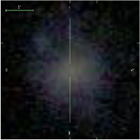
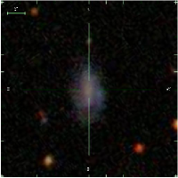
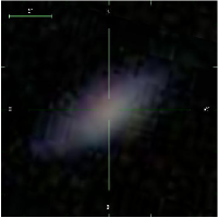
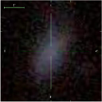
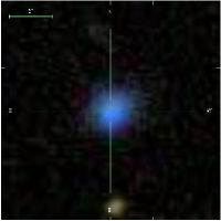
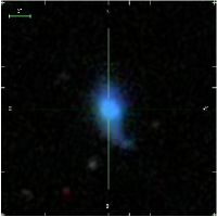
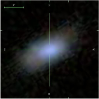
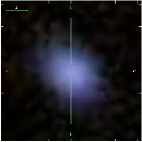
Figure 3.— Set of randomly chosen images of QBCD candidates (top) and BCD candidates (bottom). We are using the color look-up table of SDSS. Each galaxy includes a horizontal scale corresponding to 5″. The crosses centered in the galaxies point out north, south, east and west directions.

Figure 4 shows various histograms corresponding to the observed properties of this set of galaxies (the solid lines).

Figure 4.— Histograms of the observed magnitudes and colors corresponding to our selection of QBCD galaxies (the solid lines), and BCD candidates (the dotted lines). We also consider a sub-set of QBCD galaxies with large apparent size ($R_{50}>4$″). Their properties are shown using dashed lines. The labels in the ordinate axes specify the parameter that is represented – from top to bottom and left to right, absolute $z$ magnitude $M_{z}$, absolute $g$ magnitude $M_{g}$, surface brightness color $\langle\mu_{g}\rangle-\langle\mu_{r}\rangle$, surface brightness $\langle\mu_{g}\rangle$, oxygen-to-hydrogen abundance in the usual scale $12+\log({\rm O/H})$, and $H_{\alpha}$ equivalent width. The histogram of metallicities also includes the solar value for reference ($12+\log[{\rm O/H}]_{\odot}\simeq 8.91$; Kunth & Östlin 2000).

Means, standard deviations and modes corresponding to these histograms are listed in Table 2. The determination of the concentration indexes of small galaxies may be problematical. They are based on determining galaxy sizes and, therefore, they are affected by seeing (see Blanton et al. 2003a). We select a subset among the QBCD  candidates to test whether the main properties of the candidates depend on the spatial resolution. To be on the safe side, we consider candidates having $R_{50}>4$″, i.e., larger than the typical SDSS seeing ($\lesssim 1.5\arcsec$). The corresponding histograms are also shown in Fig. 4 (the dashed lines), with the means, standard deviations and modes included in Table 2. Except for the surface brightness, there are no systematic differences between the full set and the subset of large QBCD galaxies. Moreover, the decrease of surface brightness for large galaxies has nothing to do with poor seeing. It is a bias imposed by our lower limit in absolute magnitude (Table 1, 3rd row). Unless the large galaxies are also low surface brightness, they are much too bright to satisfy our selection criterion. In short, poor seeing does not seem to bias our selection in any obvious way.

Table 2Statistical properties of various galaxy sets.

Galaxy	$M_{z}$			$M_{g}$			$\langle\mu_{g}\rangle-\langle\mu_{r}\rangle$			$\langle\mu_{g}\rangle$			12+log(O/H)			$H_{\alpha}$ EW
Set							[mag arcsec-2]			[mag arcsec-2]						[Å]
	av$\pm$std	md		av$\pm$std	md		av$\pm$std	md		av$\pm$std	md		av$\pm$std	md		av$\pm$std	md
Observed QBCD	-18.5$\pm$1.1	-18.8		-17.6$\pm$0.8	-18.3		0.50$\pm$0.24	0.46		21.8$\pm$0.88	22.0		8.61$\pm$0.30	8.60		28.1$\pm$49.2	1.9
Large QBCD	-18.0$\pm$1.3	-18.6		-17.3$\pm$1.0	-18.1		0.47$\pm$0.16	0.46		22.7$\pm$0.67	22.9		8.61$\pm$0.26	8.60		19.9$\pm$35.5	9.9
Observed BCD	-17.9$\pm$1.1	-18.3		-17.5$\pm$1.1	-19.0		0.04$\pm$0.23	0.15		20.8$\pm$0.54	21.0		8.24$\pm$0.16	8.35		172.$\pm$174.	58.
Restored QBCD	-16.2$\pm$1.6	-14.9		-15.5$\pm$1.4	-14.2		0.37$\pm$0.23	0.38		22.2$\pm$0.95	22.6		8.43$\pm$0.31	8.40		33.1$\pm$50.4	1.9
Restored BCD	-16.2$\pm$1.5	-16.3		-15.8$\pm$1.4	-15.1		0.04$\pm$0.22	0.15		21.0$\pm$0.59	21.7		8.12$\pm$0.20	8.14		121.$\pm$ 64.	58.

2.2. Selection of BCD galaxies

The galaxies in § 2.1 are selected to be quiescent BCDs. It is clear that this conjecture and the galaxy properties must be examined in terms of the properties of the BCD galaxies. This is particularly true to answer the first basic question of whether the number density of QBCD candidates suffices to account for the existing BCDs. Number densities are best characterized as LFs but, to the best of our knowledge, there is no BCD LF in the literature. Moreover, even if such a LF existed, it would have been produced with a number of (unknown) biases different from those involved in our SDSS selection. Therefore, we found it necessary to extract from SDSS a set of BCD galaxies, that is to say, to construct a reference BCD sample with the biases and problems of the QBCD galaxies we want to compare to. This section describes such selection of BCD candidates.

The general criteria have been taken form Malmberg (2005), but they are implemented according to Gil de Paz et al. (2003). A BCD galaxy should have the following properties, (1) be blue enough, which constrains the colors, (2) be compact, which limits the surface brightness, (3) be dwarf, which sets a lower limit to the magnitude, (4) have a large star formation rate (SFR), which implies having enough H ii regions and, therefore, enough $H_{\alpha}$ emission, (5) be metal poor, and (6) not to be confused with AGNs. These general criteria have been specified as detailled in Table 3. The numerical values corresponding to constraints (1), (2) and (3) have been taken from Gil de Paz et al. (2003), who point out three photometric criteria for a galaxy to be a BCD,

$$\langle\mu_{B}\rangle-\langle\mu_{R}\rangle\leq{\rm~{}1~{}mag~{}arcsec}^{-2},$$

$$\langle\mu_{B}\rangle<{\rm~{}22~{}mag~{}arcsec}^{-2},$$ (6)

$$M_{K}>-21{\rm mag}.$$

Using the transformation between Johnson’s and SDSS photometric systems in Smith et al. (2002), plus equation (1) in Gil de Paz et al. (2003), these three conditions become the constraints (1), (2) and (3) in Table 3. The mean surface brightness $\langle\mu\rangle$ has been computed as the magnitude of the average luminosity within $R_{50}$, i.e., $\langle\mu\rangle=2.5\log(2\pi)+m+5\log R_{50}$, with $m$ the apparent magnitude (see, e.g., Blanton et al. 2001, § 2.3). The transformation between photometric systems is suited for stars, rather than for galaxies with emission lines like the BCDs. However, the approximation suffices because the actual limits in equation (6) are estimative, and the effect of including lines modifies the BCD magnitudes by 0.1 mag or less. This effect has been estimated using SDSS spectra representative of BCD galaxies.

Table 3Criteria used to select BCD galaxies from the SDSS/DR6 database.

#	Criterion	Implementation
(1)	Be blue enough	$\langle\mu_{g}\rangle-\langle\mu_{r}\rangle\leq 0.43$ mag arcsec-2
(2)	Be compact	$\langle\mu_{g}\rangle<21.83-0.47(\langle\mu_{g}\rangle-\langle\mu_{r}\rangle)$ mag arcsec-2
(3)	Be dwarf	$M_{g}>-19.12+1.72(M_{g}-M_{r})$ mag
(4)	Having large SFR	${H_{\alpha}}$ Equivalent Width $>50~{}$Å
(5)	Be metal poor	$12+\log({\rm O/H})<8.43$ ($\equiv$ 1/3 $\odot$)
(6)	Not to be confused with AGNs	neglect AGN contamination
(7)	Be isolated	no bright galaxy within 10 $R_{50}$
(8)	Get rid of proper motion	redshifts $>0.003$
	induced redshift

The actual implementation of criteria (4) and (5) are mere educated guesses that try not to be too restrictive. For example, we consider metallicities smaller than 1/3 the solar value (Table 3, item 5), when Kunth & Östlin (2000) bound the BCDs metallicities between 1/10 and 1/50. The (oxygen) metallicity of the galaxies (O/H) has been estimated using the so-called N2 method, based on the equivalent widths of the emission lines $[NII]\lambda 6583$ and $H_{\alpha}$,

$$12+\log({\rm O/H})=9.12+0.73\,{\rm N2},$$ (7)

with

$${\rm N2}=\log{{[NII]\lambda 6583}\over{H_{\alpha}}};$$

see Shi et al. (2005) and references therein. Note that this metallicity characterizes the properties of the H ii regions excited by the starburst, which represents only a very small fraction of the galactic gas (see § 5). Keeping the appropriate caveats in mind, the N2 method suffices for the elementary estimate we are interested in.

Active Galactic Nuclei (AGNs) can be misidentified as star-forming galaxies since they are high surface brightness blue galaxies with emission lines. AGNs introduce spurious BCD candidates. In practice, however, this contamination is negligible, and we do not decontaminate for the presence of AGNs (item 6 in Table 3). Our approach can be justified using the criterion to be an AGN by Kauffmann et al. (2003). An emission line galaxy is an AGN if

$$\log{{[OIII]\lambda 5007}\over{H_{\beta}}}>1.3+0.61/\Big{(}\log{{[NII]\lambda 6583}\over{H_{\alpha}}}-0.05\Big{)}.$$ (8)

We selected all SDSS BCD candidates chosen according to Gil de Paz et al. (2003) criteria (items 1, 2 and 3 in Table 3), and having the spectral line information required to apply the test (the lines $[OIII]\lambda 5007$, $[NII]\lambda 6583$, $H_{\alpha}$, and $H_{\beta}$). Figure 5 shows the scatter plot of the two indexes involved in equation (8). Points above the solid line are AGNs according to the criterion in equation (8). There are very few AGNs and, what is even more important, most of them stay to the right of the vertical dashed line, i.e.,

$${\rm N2}=\log{{[NII]\lambda 6583}\over{H_{\alpha}}}>-0.95,$$ (9)

which corresponds to the constraint on the N2 index imposed when the O/H abundance estimate is based on the N2 index, and the O/H is constrained as we do (item 5 in Table 3). Our BCD candidates are to the left of this line and therefore the low O/H abundance constraint automatically removes most of the AGN contamination, which explains our approach. In order to quantify the residual contamination, let us mention that only 0.4% of the low O/H abundance BCD candidates in Fig. 5 are also AGN candidates.

Figure 5.— Diagnostic plot used to identify AGNs contaminating the BCD sample. The points above the thick solid line correspond to AGNs candidates. The vertical dashed line separates the low O abundance region (to the left) and the high O region (to the right). We only use low O candidates, where the AGN contamination is minimum. The two indexes are defined in the main text.

We select isolated BCD candidates (criterion 7 in Table 3) because of consistency with the criteria used to search for BCD host galaxy candidates. As in the case of QBCDs, we stipulate that the galaxies have no bright companion within $10~{}R_{50}$, where $R_{50}$ is the radius including 50% of the Petrosian flux. The companions are not bright enough to perturb the galaxy if they are three magnitudes fainter than the galaxy.

Applying the criteria in Table 3 to the SDSS/DR6, one gets 1609 BCD galaxies. The dotted lines in Fig. 4 represent the distribution of physical properties of this set of candidates. Means, standard deviations, and modes are also included in Table 2. Four randomly chosen BCD candidates are shown in Fig. 3, bottom. The main redshift of the BCD candidates is 0.032, with a standard deviation of 0.019.

After carrying out the selection described above, we figured out that most of the BCD sample is also part of the QBCD sample: 1198 galaxies are shared by the two sets. They represent 74.5% of the BCDs and 5.6% of the QBCDs. The typical properties of the sets are very different (Table 2 and Fig. 4), however there is overlapping between the two populations. Roughly speaking, the BCD sample represents the fraction QBCD galaxies having the largest $H_{\alpha}$ equivalent width (see Fig. 4, bottom right, where the dotted line and the solid line agree for $H_{\alpha}$ EW $\gtrsim 100$ Å). Since the $H_{\alpha}$ luminosity is a proxy for star formation (e.g. Kennicutt 1998), the BCD sample seems to be the QBCDs having the largest specific Star Formation Rate (SFR), i.e., the largest SFR per unit of luminosity. The overlapping is consistent with the two galaxy sets being part of a single continuous sequence, the most active QBCD galaxies still being identified as BCD galaxies.

3. Luminosity functions

The LF, $\Phi(M)$, is defined as the number of galaxies with absolute magnitude $M$ per unit volume and unit magnitude. We will use it to quantify the number of QBCD candidates per BCD galaxy existing in the nearby universe. LFs are computed using a maximum likelyhood procedure similar to the methods described in the literature (e.g., Efstathiou et al. 1988; Lin et al. 1996; Takeuchi et al. 2000; Blanton et al. 2001). We developed and tested our own code for training purposes, and its characteristics and similitude with existing methods are described in App. A. Cubic splines are used to parameterize the LF shape, and the best fit is retrieved maximizing the likelyhood in equation (A9), a task realized with the usual Powell algorithm (e.g. Press et al. 1988). Errors bars are assigned by bootstrapping.

When the procedure is applied to the QBCD galaxies described in § 2.1, one finds the LF represented in Fig. 6a (the solid line).

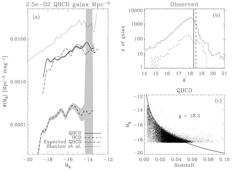
Figure 6.— (a) $g$ color LFs of the QBCD galaxy sample (the solid line), and the BCD galaxy sample (the dashed line). The shaded area shows our statistical error estimate. The dotted-dashed line represents the LF to be expected when the starburst of the BCD galaxies fades away revealing the underlying host galaxies. The dotted line corresponds to the LF of low luminosity galaxies by Blanton et al. (2005), and it is shown here for reference. (b) Observed apparent magnitudes $g$, with the vertical lines corresponding to the magnitude limits used to derive the LFs. As the inset in (a) indicates, the solid line and the dashed line represent the QBCD sample and the BCD sample, respectively. (c) Scatter plot of the absolute magnitude of the QBCD galaxies vs the redshift. The solid line shows the boundary to be expected if the sample were limited in magnitude with $g<18.3$.

This LF is similar to that obtained with the $1/V_{\rm max}$ method working on the same data sets (see App. A). The formal errors deduced from bootstrapping are very small (the shaded area around the solid line in Fig. 6a). We use 50 bootstrap re-samples, but the error estimate is not very sensitive to this parameter. The LF is mostly sensitive to the apparent magnitude limit of the QBCD galaxy set. We are using a single apparent magnitude limit for the full dataset, and changing this limit modifies the overall normalization – given a number of observed galaxies, the deeper the magnitude limit the lower the inferred number density of galaxies. We take for the limit,

$$g<18.3.$$ (10)

This selection is consistent with the magnitude limit of the main SDSS galaxy sample ($r<17.8$, Adelman-McCarthy & the SDSS collaboration 2007), keeping in mind that the QBCD galaxies are somewhat red with $g-r\simeq 0.5$ (see Table 2 and Fig. 4). However, we obtain the limit in equation (10) from the scatter plot of the QBCD galaxy absolute magnitude vs the redshift shown in Fig. 6c. By trial and error, we modify the curve representing the boundary to be expected if the whole sample were limited with a single apparent magnitude. The best match is shown as the solid line in Fig. 6c and, except for the range of large luminosities, the data set fits in well the expected behavior. Galaxies whose apparent magnitudes exceed the threshold in equation (10) are not used to compute the LF – a histogram of the observed apparent magnitudes is shown in Fig. 6b (the solid line). The normalization of the LF depends on the fraction of sky covered by survey, which we take to be the coverage of the SDSS/DR6 spectroscopic catalog (7425 deg²; Adelman-McCarthy & the SDSS collaboration 2007).

Figure 6a also shows the LF corresponding to the BCD galaxies selected in § 2.2 (the dashed line). The number density of BCD candidates ($n_{0~{}\rm BCD}\simeq 9.2\,10^{-4}$ Mpc^-3) is much smaller than the number density of QBCD galaxies ($n_{0~{}\rm QBCD}\simeq 2.5\,10^{-2}$ Mpc^-3), giving,

$${{n_{0~{}\rm QBCD}}\over{n_{0~{}\rm BCD}}}\simeq 27.$$ (11)

In this case the limit magnitude of the sample has been set to $g<18.5$, which we determine with the same procedure used for the QBCD galaxies. The need for a different apparent magnitude limit can be inferred from the histograms in Fig. 6b. Note how the histogram for BCD galaxies (the dashed line) does not drop off for large magnitudes as abruptly as the histogram for the QBCD galaxies (the solid line).

The calculus of LFs has been repeated using $z$ magnitudes, i.e., the redder SDSS color filter at $9097~{}$Å. This bandpass is less sensitive to (blue) starbursts, enhancing the contribution of old stellar populations. The results are represented in Fig. 7.

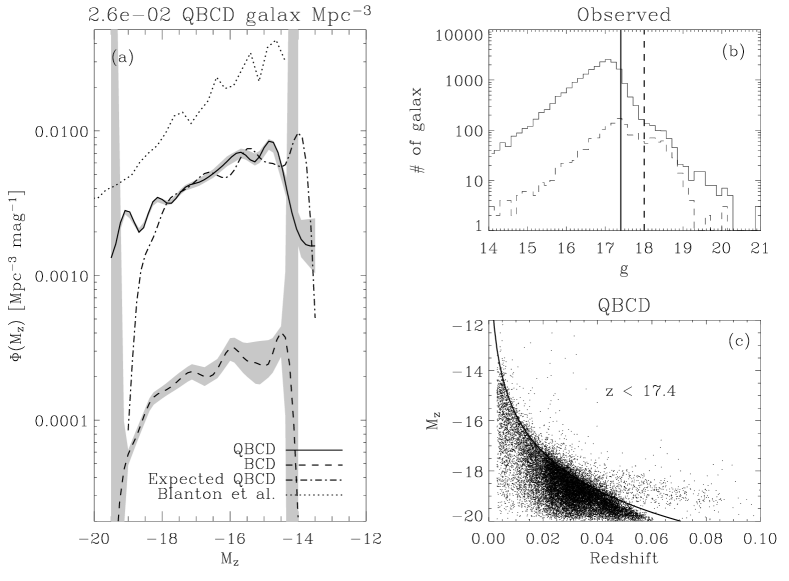
Figure 7.— This figure is identical to Fig. 6 except that the LFs, the histograms, and the scatter plot refer to $z$, i.e., the redder color among the SDSS bandpasses. See Fig. 6 caption for details.

They are similar to those obtained from $g$, except that the LFs are shifted by one magnitude. The ratio between the number of QBCD galaxies and BCD galaxies remains as in equation (11) – 24 in this particular case.

Figures 6a and 7a include the LFs for extremely low luminosity galaxies worked out by Blanton et al. (2005) (the dotted lines). We used them as a reference, since they include all low redshift galaxies in the SDSS spectroscopic catalog and, therefore, they provide LFs for the local universe affected by the same kind of bias as our galaxy selection. Using these LFs as reference, we find the QBCD galaxies to be rather numerous. One out of each three dwarf galaxies is a QBCD candidates (cf. the solid lines and the dotted lines in Figs. 6a and 7a). Similarly, one out of each ninety dwarf galaxies is a BCD candidate (cf. the dashed lines and the dotted lines in Figs 6a and 7a).

Our LFs are not corrected for the incompleteness of the SDSS catalog at low surface brightness. According to the detailled simulation carried out by Blanton et al. (2005, Fig. 3), the incompleteness is not significant for galaxies with $\langle\mu_{g}\rangle<23.5$. Most of our QBCD candidates are within this bound (Fig. 4, bottom left), and it does not affect the BCD selection at all (Table 3). The QBCD LF would be affected at its faint end, but even at $M_{g}\sim-14$ the expected correction is not larger than a factor of two (Blanton et al. 2005, Fig. 6). This uncertainty does not modify the conclusions of the paper, which are mostly qualitative. However, the number of QBCD galaxies worked out in the paper may be underestimated by a factor of order one.

3.1. From LF of BCDs to LF of BCD hosts

The question arises as to whether the LFs for QBCD galaxies and BCD candidates are consistent. They seem to be, according to the following heuristic procedure to estimate the LF for the hosts of the BCDs. Given a LF of BCDs, $\Phi_{\rm BCD}$, one can work out the LF to be expected once the starburst dies out, $\Phi_{\rm QBCD}$. By switching the star formation on and off, BCD galaxies turn into QBCD galaxies, and vice versa. These two evolutionary phases have different timescales; $\tau_{\rm BCD}$ for the BCD phase, and $\tau_{\rm QBCD}$ for the QBCD phase. In a stationary state the number of galaxies turning from BCD to QBCD must be balanced by the galaxies going from QBCD to BCD,

$$\Phi_{\rm QBCD}(M){{\Delta M}\over{\tau_{\rm QBCD}}}\simeq\Phi_{\rm BCD}(M^{\prime}){{\Delta M^{\prime}}\over{\tau_{\rm BCD}}},$$ (12)

where BCD galaxies with magnitude in the interval $M^{\prime}\pm\Delta M^{\prime}/2$ become QBCD galaxies with magnitudes $M\pm\Delta M/2$. Combining equation (12) with the empirical relation between the magnitudes of the host galaxy and the BCD (equation [1]), one has the recipe to infer the LF of the host galaxies to be expected from the LF of the BCD galaxies,

$$\Phi_{\rm QBCD}(M)\simeq{{\tau_{\rm QBCD}}\over{\tau_{\rm BCD}}}\Phi_{\rm BCD}(M-0.5).$$ (13)

The scaling factor $\tau_{\rm QBCD}/\tau_{\rm BCD}$ is just the ratio between the number densities of BCDs, $n_{0~{}\rm BCD}$, and QBCDs, $n_{0~{}\rm QBCD}$,

$${{\tau_{\rm QBCD}}\over{\tau_{\rm BCD}}}\simeq{{n_{0~{}\rm QBCD}}\over{n_{0~{}\rm BCD}}},$$ (14)

since $\Phi_{\rm QBCD}$ and $\Phi_{\rm BCD}$ are normalized to $n_{0~{}\rm QBCD}$ and $n_{0~{}\rm BCD}$, respectively.

Using equations (13) and (14), we evolve the LF of BCD galaxies in Figs. 6a and 7a to obtain the LFs of their host galaxies. They are included in the same figures as the dotted-dashed lines. The scaling (14) has been taken as the ratio between the number densities of QBCD galaxies and BCD galaxies (i.e., the ratio in equation [11] for the $g$ filter, and the corresponding figure for the $z$ filter). The similarities between the evolved LF (the dotted-dashed lines) and the LF computed from the QBCD data sets (the solid lines) are quite striking. We interpret this agreement as an indication of self-consistency between the two sets of galaxies chosen in § 2. BCD galaxies and QBCD galaxies can be different phases in the life of a dwarf galaxy, with the lifetime in the BCD phase some thirty times shorter than the lifetime in the QBCD phase (equations [11] and [14]).

The BCD starbursts are very young since they still conserve massive stars (see § 1). If $\tau_{\rm BCD}\simeq 10~{}$My then equations (14) and (11) imply $\tau_{\rm QBCD}\simeq 0.27~{}$Gy. Consequently, each QBCD galaxy may undergo as many as 30-40 star formation episodes during the timespan where stars can be formed in dwarf galaxies ($\gtrsim$10 Gy; e.g., Kunth & Östlin 2000). This issue is discused in § 5.

4. Properties of QBCD galaxies and BCD galaxies

The histograms of galaxy properties discussed in § 2, and shown in Fig. 4, describe the properties of the observed galaxies. These histograms are strongly biased since they overweight the properties the most luminous galaxies in the samples. In order to correct for the Malmquist bias, so that histograms are weighted according to the true number density of galaxies, we have used the ratio between the LF derived in § 3, $\Phi(M)$, and the observed histogram of absolute magnitudes,

$$h(M)={1\over{\Delta M}}\sum_{i}\,\Pi\big{(}{{M_{i}-M}\over{\Delta M}}\big{)}.$$ (15)

As usual, the symbol $\Pi$ stands for the rectangle function,

$$\Pi(x)=\cases{1&$|x|<1/2$,\cr 0&elsewhere.}$$ (16)

The index $i$ in equation (15) includes all observed galaxies, whereas $M$ and $\Delta M$ determine the centers and the widths of the histogram bins . We have to assume that each observed galaxy is actually a proxy for $b_{i}$ galaxies, $b_{i}-1$ of which are not included in our observation because they are too faint to exceed the apparent magnitude threshold. The magnitude of the galaxy causes the bias and, therefore, we assume that the bias function only depends on the absolute magnitude of the galaxy,

$$b_{i}=b(M_{i}).$$ (17)

This bias is precisely the reason why $h(M)$ is not the LF, therefore, for $\Delta M$ small enough,

$$\Phi(M)\simeq{1\over{\Delta M}}\sum_{i}\,b_{i}\,\Pi\big{(}{{M_{i}-M}\over{\Delta M}}\big{)}.$$ (18)

Using equation (17), and assuming that $b(M)$ is a slowly varying function of $M$,

$$b(M_{i})\,\Pi\big{(}{{M_{i}-M}\over{\Delta M}}\big{)}\simeq b(M)\,\Pi\big{(}{{M_{i}-M}\over{\Delta M}}\big{)},$$ (19)

and so one finds from equation (18) the expression for the bias function,

$$b_{j}=b(M_{j})=\Phi(M_{j})/h(M_{j}).$$ (20)

Let us denote as $k(p)$ the histogram of any parameter $p$ constructed using the observed galaxies,

$$k(p)={1\over{\Delta p}}\sum_{i}\,\Pi\big{(}{{p_{i}-p}\over{\Delta p}}\big{)},$$ (21)

with $\Delta p$ the bin-size and $p_{i}$ the value corresponding to the $i$-th galaxy. Then the bias-corrected histogram would be,

$$k^{*}(p)={1\over{\Delta p}}\sum_{i}\,b_{i}\,\Pi\big{(}{{p_{i}-p}\over{\Delta p}}\big{)}.$$ (22)

This definition guarantees that the corrected histogram of observed absolute magnitudes is the luminosity function (cf. equations [18] and [22] with $p=M$) and, therefore, it is not difficult to show that all corrected histograms have the same normalization as the LF, i.e.,

$$\int_{-\infty}^{\infty}k^{*}(p)\,dp=n_{0},$$ (23)

$n_{0}$ being the number density of galaxies (see App. A).

We have applied equations (20) and (22) to restore the histograms in Fig. 4. The result is shown in Fig. 8. The means, standard deviations and modes of the new histograms are also included in Table 2. As expected, the mean absolute magnitudes of the restored histograms are much fainter than the observed ones. However, in addition to this effect, the corrected histograms hint at intrinsic metallicities significantly lower than the observed ones both for BCD and QBCD galaxies. The corrected QBCD galaxy colors are bluer than the colors of the observed set.

Figure 8.— Histograms of magnitudes and colors for QBCDs (the solid lines) and BCDs (the dotted lines) once the Malmquist bias has been compensated for. The unrestored versions of these histograms are shown in Fig. 4. The labels in the ordinate axes describe the parameter that is represented. The histograms are normalized to the number density of galaxies. The dashed line in the plot of metallicities ($12+\log[{\rm O/H}]$) reproduces Fig. 3 in Kunth & Östlin (2000), which corresponds to the abundances of 425 H ii galaxies cataloged by Terlevich et al. (1991). Refer to Fig. 4 for further details.

These changes can be pin down to the correlations between luminosity, color, and metallicity existing in the original data set. Figure 9 shows how the QBCD galaxies tend to be less metallic as they become fainter, and a similar, but less marked trend, is also present in BCD galaxies. Such a relationship between metallicity and mass in dwarf galaxies (and so, between metallicity and luminosity) was given by Pagel & Edmunds (1981), and later on by many others (see Kunth & Östlin 2000). Figure 9 includes the linear relationship found by Skillman et al. (1989) for nearby dwarf irregular galaxies. Curiously enough, the slope is almost the same as we find for QBCD galaxies. There is also a relationship between color and luminosity, so that fainter QBCD galaxies seem to be bluer; see Fig. 10.

Figure 9.— Metallicity vs absolute $M_{g}$ magnitude. The symbols stand for the mean values considering all the galaxies with similar $M_{g}$, whereas the error bars represent the standard deviation of the mean values. Both QBCD galaxies (the square symbols) and BCD galaxies (the asterisks) follow a trend so that the fainter the galaxy the more metal poor. The solid line is shown for reference and it corresponds to the law for nearby dwarf irregular galaxies found by Skillman et al. (1989).

Figure 10.— $\langle\mu_{g}\rangle-\langle\mu_{r}\rangle$ color vs absolute $M_{g}$ magnitude. The symbols stand for the mean values considering all the galaxies with similar $M_{g}$, whereas the error bars represent the standard deviation to be expected for these mean values. The QBCD galaxies are bluer as they become fainter (the square symbols). The same trend is not so obvious for the BCD galaxies (the asterisks).

Figures 9 and 10 actually reveal an underlying relationship between color and metallicity. It has been brough up in Fig. 11, showing how the redder the galaxy the larger the oxygen abundance. The relationship is more clear in the case of the QBCD galaxies (the square symbols), but it is also present among the redder BCD galaxies (the asterisks for $\langle\mu_{g}\rangle-\langle\mu_{r}\rangle>-0.4$). The relationships for QBCDs and BCDs meet at $\langle\mu_{g}\rangle-\langle\mu_{r}\rangle\simeq-0.1$, although they have different slopes.

Figure 11.— Metallicity vs color. There is a clear trend, which becomes steeper and sharper in the case of the QBCD galaxies (the square symbols). The solar metallicity has been marked for reference. Each symbol represents the average metallicity ($12+\log[{\rm O/H}]$) considering all the galaxies with the same color. The error bars correspond to the standard deviation to be expected for these averages.

The number of known BCD galaxies with metallicities less than 1/20 the solar value is rather small (a dozen or so, according to Kunth & Östlin 2000). Surprisingly enough, the list of 1609 BCD candidates we work out contains only three candidates below this metallicity. We interpret this result as a support of the metallicity estimate carried out in the paper, but it also reinforces the existence of a minimum H ii region based metallicity (see Kunth & Östlin 2000, and references therein).

The range of selected QBCD colors is rather broad and, therefore, our list of QBCD candidates seems to include all the range from early-type galaxies to late-type galaxies. This fact can be appreciated in Fig. 12a, which contains a color-color scatter plot. Our galaxies follow the sequence used in galaxy classification, with the reddest extreme corresponding to elliptical galaxies (early types), and the bluest extreme to irregular galaxies (late types) – compare Fig. 12a with, e.g., Fig. 2 in Bershady et al. (2000). One can distinguish two clusters or concentrations in Fig. 12a (the dashed line arbitrarily separates the two sub-sets). The existence of these two clusters or classes was to be expected, since they correspond to the bimodal distribution of colors found in the large samples of galaxies (e.g., Balogh et al. 2004; Blanton et al. 2005). Hints of these two modes are also found as two small peaks in the histogram of surface brightness color shown in Fig. 4 (top right, the solid line, with the two peaks at $\langle\mu_{g}\rangle-\langle\mu_{r}\rangle\simeq$ 0.4 and 0.7). Note how the BCD candidates occupy the bluest extreme of the color-color plot; cf. Figs. 12a and 12b.

Figure 12.— (a) $u-g$ vs $g-r$ scatter plot for the QBCD candidates. The colors in the sequence span from those of early-type galaxies, to those of late-type galaxies. There seem to be two clusters in the distribution of points, which we have artificially separated by the dashed line. (b) Same as (a) but showing the BCD candidates.

Most of the QBCD candidates show $H_{\alpha}$ in emission, meaning that even if the star-formation is reduced with respect to the BCD candidates, it is not absent. Only some 3200 QBCD galaxies out of the 21493 candidates show $H_{\alpha}$ in absorption. They have (negative) equivalent widths of a few Å and, therefore, these objects are included in the bin of zero equivalent width in Fig. 4, bottom right. Using the $H_{\alpha}$ flux as a proxy for star formation (Kennicutt 1998), our QBCD candidates turn out to be one order of magnitude less active in forming stars than the BCDs. This estimate is worked out in § 5.1, equations (28) and (29).

5. Discusion

So far we have described our search avoiding interpreting the results. This section, however, is fully devoted to interpretation and so, admittedly speculative. We will discuss how the results in previous sections are consistent with the BCD candidates and the QBCD candidates being two different phases in the same sequence of galactic evolution. Using as a working hypothesis that BCDs change into QBCDs, and vice versa, we examine obvious flaws and constraints. Showing the consistency of an hypothesis does not prove it to be correct – other alternatives cannot be discarded. It just shows the working hypothesis to be viable. Three main results point out in this direction. First, we choose the QBCDs so that their colors, concentration indexes and luminosities are equal to those of the galaxies underlying the BCDs. Second, the LF of QBCDs is conformable to the LF of BCDs (§ 3). Third, the BCD galaxies turn out to be QBCD galaxies with the largest (specific) star formation rates (§ 2.2).

Matching LFs forces the QBCD phase to last some 30 times longer than the BCD phase (§ 3.1). Since the BCD starbursts are so short-lived, there should be many episodes of BCD phase during a galaxy lifetime. Assuming a single 10 My long starburst per BCD phase, there should be one of such BCD phases each 0.3 Gy. Longer BCD phases are in principle possible by concatenation of starbursts, but population synthesis modeling of BCD spectra does not favor extended periods of star-formation (e.g., Mas-Hesse & Kunth 1999). If BCDs are transformed into QBCDs and vice versa, each QBCD has experienced several BCD phases because the other alternative does not seem to be consistent with the results of the search. Let us examine this alternative possibility, namely, that the BCD phase represents the only episode of intense star formation during the galaxy lifetime. Statistically, all QBCD galaxies that we detect today have sufferred a BCD episode during the last 270 My (equations [11] and [14], with $\tau_{{\rm BCD}}=$10 My). If this is the only such episode per galaxy, there should be no BCDs among galaxies observed at lookback times larger than 270 My, or at redshifts $>0.02$ (= $270~{}{\rm My}/H_{0}$). However, a large fraction of the sample of BCDs selected in § 2.2 has redshifts larger than this limit. We are forced to conclude that the same host galaxy undergoes several BCD phases.

Although the recursive BCD phase scenario explains a number of important observables, other properties of QBCDs and BCDs do not seem fit in the picture so well. The purpose of the rest of the section is to discuss (and hopefully clarify) some of the most obvious difficulties posed by the scenario.

5.1. H i consumption timescale

One may think that the repeated starbursting of a dwarf galaxy quickly exhausts the gas reservoir, thereby making the whole picture inconsistent. However, the low surface brightness galaxies like the QBCDs are gas-rich (Staveley-Smith et al. 1992; Kunth & Östlin 2000), with fuel to power the star formation during several Hubble times. This claim can be supported by working out the H i consumption timescale, $\tau_{{\rm H\,I}}$, which is defined as the time required to transform into stars the neutral hydrogen of the galaxy, $M_{{\rm H\,I}}$, i.e.,

$$\tau_{{\rm H\,I}}=M_{{\rm H\,I}}/{\rm SFR},$$ (24)

with SFR the star formation rate. On the one hand, dwarf low surface brightness galaxies have about one solar mass of H i per solar luminosity (Staveley-Smith et al. 1992), explicitly,

$$\log(M_{{\rm H\,I}}/M_{\odot})=-0.4\,(M_{g}-M_{g\,\odot}),$$ (25)

$M_{\odot}$ being one solar mass, and $M_{g\,\odot}$ the solar absolute luminosity in the $g$ filter. On the other hand, the SFR scales with the $H_{\alpha}$ luminosity (e.g., Kennicutt 1998), i.e., with the product of the $H_{\alpha}$ equivalent width times the galaxy luminosity. Since the observed BCD $H_{\alpha}$ equivalent width is uncorrelated with the galaxy luminosity, the BCD SFR scales with the luminosity, that is to say,

$$\log({\rm SFR_{BCD}/SFR^{\prime}_{BCD}})=-0.4(M_{g}-M_{g}^{\prime}),$$ (26)

where ${\rm SFR^{\prime}_{BCD}}$ stands for the SFR of a BCD galaxy of magnitude $M_{g}^{\prime}$. In our two-phase scenario, the galaxy has short periods of star formation lasting $\tau_{\rm BCD}$, interleaved with long periods of quiescence lasting $\tau_{\rm QBCD}$ (§ 3.1). Consequently, the effective time-average SFR is,

$${\rm SFR}\simeq{{\tau_{\rm BCD}\,{\rm SFR_{BCD}}+\tau_{\rm QBCD}\,{\rm SFR_{QBCD}}}\over{\tau_{\rm BCD}+\tau_{\rm QBCD}}}$$ (27)

$$\simeq{\rm SFR_{BCD}}\Large({{\tau_{\rm BCD}\over{\tau_{\rm QBCD}}}}+\epsilon\large),$$

with

$$\epsilon={{\rm SFR_{QBCD}}\over{\rm SFR_{BCD}}}.$$ (28)

As judged from the ratio of $H_{\alpha}$ equivalent widths in Table 2, and the difference of luminosity between BCDs and QBCDs (equation [1]), the SFR during the BCD phase is some ten times larger than during the QBCD  phase, i.e.,

$$\epsilon^{-1}\simeq 10.$$ (29)

By combining equations (24), (25), (26) and (27), one finds the consumption timescale to be independent of the galaxy luminosity,

$$\log\tau_{{\rm H\,I}}\simeq-0.4(M_{g}^{\prime}-M_{g\,\odot})-\log\Big{[}{{\rm SFR_{BCD}^{\prime}}\over{M_{\odot}}}\big{(}{{\tau_{\rm BCD}}\over{\tau_{\rm QBCD}}}+\epsilon\big{)}\Big{]}.$$ (30)

Although BCD star formation bursts are intense for a dwarf galaxy, the SFRs of BCDs are rather modest, i.e., less than $1M_{\odot}{\rm y}^{-1}$, and typically one order of magnitude smaller (e.g. Sage et al. 1992; Mas-Hesse & Kunth 1999). Taking ${\rm SFR}^{\prime}_{\rm BCD}<1M_{\odot}{\rm y}^{-1}$ for the brightest galaxies of our sample, $M_{g}^{\prime}\simeq-19$, and using the ratio of timescales between the phases as provided by equations (11) and (14), equations (29) and (30) yield,

$$\tau_{{\rm H\,I}}\gtrsim 30~{}{\rm Gy}.$$ (31)

Consequently, the hydrogen existing in QBCD galaxies allows the sequence BCD-QBCD to last for a few Hubble times ($\equiv 1/H_{0}=$14 Gy).

A final comment is in order. The scenario of a recursive starbursting is not in conflict with the commonly accepted view of a SFR decreasing during the last 10 Gy (Madau et al. 1996; Lilly et al. 1996). This drop refers to massive galaxies. However, the kind of dwarf galaxies in our QBCD sample, with stellar masses less than $10^{10}~{}M_{\odot}$, has maintained a SFR either stationary or slightly increasing with time (see Heavens et al. 2004, Fig. 1).

5.2. Metallicities

The metallicities of our QBCD galaxies are systematically larger than the metallicities of the BCD galaxies. This result seems to be in conflict with the recursive BCD phase scenario, since the BCD starburst starts off with a metallicity lower than the metallicity of its host galaxy (see Table2). Although this disagreement may indicate a real flaw in the overall picture, one can also think of various ways to circumvent the apparent inconsistency. For example, the BCD episodes may involve fresh low metallicity gas accreted by the host galaxy during the periods of quiescence. Note that the BCD episodes are very conspicuous from the point of view of the luminosity, but they involve moderate masses, which hardly exceed $10^{6}\ M_{\odot}$ (e.g. Mas-Hesse & Kunth 1999). A sustained infall such as those postulated in the literature to solve various problems in galaxy evolution ($\sim\,1M_{\odot}~{}{\rm pc}^{-2}~{}{\rm Gy}^{-1}$; see Dalcanton 2007, and references therein) provides $10^{6}\ M_{\odot}$ in only 50 My, even for a small 2.5 kpc galaxy. Masses of $10^{6}\ M_{\odot}$ are also typical of the high velocity clouds hounding our galaxy (e.g., Wakker et al. 2007). If these gas reservoirs are common in QBCDs, they may develop major star formation events when merging with the galaxy.

The fresh gas glowing during the BCD phase does not necessarily have to come from outside. Metal-poor gas may exist in place in the galaxy (§ 5.1). Then the oxygen metallicity assigned here to QBCD galaxies may not reflect the metallicity of this gas, but the metallicity of a few metal-polluted H ii regions remaining from the last starburst. It is relatively easy to enrich with metals the small fraction of galactic gas undergoing starbursts. For example, the metallicity of a pure gas cloud increases from the level observed in BCDs ($12+\log(O/H)\simeq 8.24$; Table 2) to the level in QBCDs ($\simeq 8.61$), if 60% of the original mass is transformed into starts. The metal-polluted gas produces emission lines during the extended recombination phase of the H ii region (e.g., Beltrametti et al. 1982), and it may also give rise to a secondary generation of stars. The light from these aging H ii regions renders high metallicity measurements. Eventually, the star-processed gas mingles with the metal-poor gas of the galaxy, but this mixing leaves the original metallicity almost unchanged. We note that this explanation may be in conflict with the IR excess detected in the halos of Blue Compact Galaxies by Bergvall & Östlin (2002). These halos can be identified with the BCD host galaxies and, therefore, with the QBCDs. The colors cannot be explained with a normal metal-poor stellar population like the Milky Way halo, but an excess of low-mass stars with significant metallicity is required (see Zackrisson et al. 2006). The nature of the disagreement requires further investigation, and it may be due to the fact that these Blue Compact Galaxies with IR excesses are not dwarfs according to the criteria used in our work.

There is yet another possibility to reconcile the metallicities of the two galaxy types. Only those QBCD candidates with metallicity similar to that of the BCD galaxies would be part of the BCD – QBCD sequence. The QBCDs with metallicity like the BCDs represent 20% of the sample (see Fig. 4) and, therefore, the timescale of quiescence must be shortened by a factor of five to comply with equation (14). The same happens with the H i consumption timescale worked out in equation (31). These QBCD galaxies may keep their low metallicity levels because the metals are expelled by galactic winds (Heckman 2002; Tenorio-Tagle et al. 2003; see, however, Silich & Tenonio-Tagle 2001; Legrand et al. 2001), because they are recycled into new stellar generations within superstar clusters, without significant mixing with the galactic gas (Tenorio-Tagle et al. 2005), or simply because of the dilution with pristine gas described above.

5.3. Starburst triggering

We select isolated QBCD galaxies, therefore, the starburst triggering mechanism to turn them into BCDs cannot be galaxy-galaxy interactions, mergers or harassment. How, then, are the BCD bursts triggered? Several possibilities are available. If the fresh gas falls on the QBCD galaxy over extended periods of time, intense star formation cannot be triggered until the gas density exceeds the required threshold (the so-called Schmidt law; Schmidt 1959). Waiting for enough gas to accumulate could explain periods of latency. If the gas falls in during short episodes (like the collision with a large gas cloud), the hitting of the gas itself may induce star formation. Then the QBCD timescale would be given by the characteristic time between cloud collisions. If rather than coming from outside, the fresh gas is part of the galaxy, internal galactic structures like bars may periodically excite star formation. In the case of a gas-rich galaxy the triggering may also be due to perturbations of the galactic material by dark matter clumps. These elusive structures are predicted in lots by the cold dark matter simulations of galaxy formation (e.g., Diemand et al. 2007), and they are expected to disturb the quiet evolution of galactic disks (e.g., Kazantzidis et al. 2007).

5.4. QBCD characterization criteria

The criteria used to characterize QBCDs come from the BCD host galaxies analyzed by Amorín et al. (2007, 2008), but we may have used different criteria taken from other works. The question arises as to whether the selection of candidates critically depends on this assumption.

The BCD host galaxy properties are used to constrain colors and Sersic indexes (see § 2.1 and Table 2). The lower limit luminosity, also taken from the BCD host galaxies, turns out to be unimportant since the small number low luminosity objects prevents any serious influence of this criterion on the selection (see Fig. 4). The range of visible $g-r$ colors that we use agrees with the colors that different studies have assigned to the hosts of BCDs (e.g., Papaderos et al. 1996b; Gil de Paz & Madore 2005), even in those cases where a significant infra-red excess has been detected (e.g., Bergvall & Östlin 2002). In this sense the color criterion does not seem to be questionable and, therefore, any work would have rendered similar QBCD candidates. The selection of Sersic indexes is more influential. Studies like Bergvall & Östlin (2002) or Gil de Paz & Madore (2005) find indexes as large as $n=$10–20, whereas we take $n<3$ (Table 2). However, there are two good reasons to prefer low$-n$ values. First and most important, the observed dwarf galaxies present low$-n$ values (e.g., Fig. 11 in Caon et al. 2005; Graham & Guzmán 2003), and if we search for galaxies that may be Blue-Compact-Dwarf galaxies during quiescence, they must be dwarfs too (see equation [1].) Second, the large $n$ values are obtained from 1D fits to azimuthally averaged luminosity profiles, and the $n$ thus obtained depends critically on the range of radii used to characterize the galactic outskirts (e.g., Cairós et al. 2003; Gil de Paz & Madore 2005). The 2D fits providing low indexes are fairly more robust and, therefore, to be preferred (see Amorín et al. 2007).

6. Conclusions

The starburst characteristic of BCD galaxies does not last for long. Once this episode is over, the BCD galaxies should dim their surface brightness to become quiescent BCD galaxies (or QBCD galaxies). Although QBCD galaxies are to be expected, they have not been identified yet (see § 1). The present work describes an effort to find them among the galaxies in the SDSS/DR6 database. The properties of the QBCDs have been taken from the sample of BCD host galaxies characterized by Amorín et al. (2007, 2008) (§ 2.1). We find 21493 QBCD candidates, therefore, QBCDs seem to be fairly common in the local universe. In order to have a proper reference to compare with, a complete sample of BCD galaxies was selected too. It comprises 1609 BCD candidates (§ 2.2). Since the two samples were selected from the same database using analogous criteria, the comparison between the two sets is relatively free from the bias that our selection may have.

We compute Luminosity Functions (LFs) for the two samples (§ 3). In addition, we estimate their main properties before and after correcting for Malmquist bias. These properties can be summarized as follows,

• There are around 30 QBCD candidates per BCD candidate. We infer this ratio by comparison of the LFs for QBCDs and BCDs. The two LFs are very similar, except for the global scaling factor, and the expected 0.5 magnitude dimming (§ 3.1).

• The surface brightness of the QBCDs is typically one magnitude fainter than the surface brightness of BCDs (Table 2).

• QBCD candidates are, on average, 0.4 magnitudes redder than the BCD (Table 2; $\langle\mu_{g}\rangle-\langle\mu_{r}\rangle$).

• QBCD candidates have an H ii region based oxygen metallicity 0.4 dex higher than the BCD candidates (Table 2).

• The QBCD  metallicity increases with the luminosity, following the well known trend for dwarf galaxies.

• The QBCD  metallicity also increases with the color, so that the redder the galaxy the larger the measured metallicity.

• 75 % of the BCD candidates are also part of the QBCD sample (§ 2.2). Roughly speaking, the BCD sample represents the fraction QBCD galaxies having the largest specific SFR (SFR per unit of luminosity).

• There are around three dwarf galaxies per QBCD candidate (§ 3), which renders one BCD galaxy every ninety dwarf galaxies.

The overlap between BCD galaxies and QBCD galaxies is consistent with the two sets forming a single continuous sequence, with the most active QBCD galaxies being BCD galaxies. The agreemet between their LF shapes, and the ratio of number their densities, support the commonly accepted view that BCD galaxies undergo short bursts of star formation separated by long quiescent epochs. However, the fact that the QBCD metallicity is higher than the BCD metallicity poses a problem to such an episodic starbursting scenario, which we try to circumvent with various plausible explanations in § 5.2.

The repeated starbursting scenario predicts a number of independent observables whose testing is important but goes beyond the scope of the paper. They represent a natural extension of the present work. In order to illustrate the possibilities, we will outline two examples. QBCDs must have a stellar population corresponding to short star formation episodes in between quiescent gaps. In principle, one can distinguish between a (low level of) continuous star formation and a more violent episodic star formation with a period of 0.3 Gy. Leonardi & Rose (1996) put forward a spectroscopic index to detect post-starburst galaxies. The technique is well suited for determining the time elapsed from the last (young) starburst, and it has been calibrated by Leonardi & Worthey (2000). Depending on the noise level, one can apply the method to selected QBCD SDSS spectra, or to averages of similar QBCD spectra. Another testable prediction of the scenario has to do with the metallicity inferred from emission lines in QBCD galaxies (§ 5.2). It should overestimates the true galaxy metallicity and, in particular, the metallicity of the stellar content. Studies of stellar metallicity can be carried out using integrated galaxy spectra, provided that they have enough signal-to-noise ratio and spectral resolution to show absorption lines (e.g. Terlevich et al. 1990; Worthey et al. 1994). These two testable predictions provide a flavor for other tests to come.

Appendix A Luminosity function estimate

The LF, $\Phi(M)$, is defined as the number of galaxies with absolute magnitude $M$ per unit of magnitude and unit of volume. We use it to describe the local universe and, therefore, $\Phi(M)$ is not expected to change with the position in space. The number of galaxies per unit volume, $n_{0}$, is just,

$$n_{0}=\int_{M_{l}}^{M_{u}}\Phi(M)\,dM,$$ (A1)

where only absolute magnitudes in between the limits $M_{l}\leq M\leq M_{u}$ are considered. Using the definition of LF, one can easily write down the number of galaxies to be expected in an apparent magnitude limitted catalog, namely,

$$N=\int_{M_{l}}^{M_{u}}\Phi(M)\,V_{\rm max}(M)\,dM.$$ (A2)

As usual, the symbol $V_{\rm max}(M)$ stands for the volume of universe covered by the catalog where galaxies of absolute magnitude $M$ have apparent magnitudes smaller than the catalog threshold (e.g., Takeuchi et al. 2000).

Maximum likelyhood estimates of LFs are favored in the current literature (e.g., Lin et al. 1996; Blanton et al. 2001). They were pioneered by Efstathiou et al. (1988) and, among the quoted advantages, they present a number of desirable asymptotic error properties. Note, however, that these methods are not unbiased (the expected value of the estimate is not necessarily the parameters to be estimated). The method is based on the following principle; given the redshift $\zeta$ of an observed galaxy, the probability that it has an absolute magnitude $M$ is,

$$P(M\,|\,\zeta)=\Phi(M)\Big{/}\int^{M_{\rm max}(\zeta)}_{M_{\rm min}(\zeta)}\Phi(M^{\prime})\,dM^{\prime},$$ (A3)

where the normalization gives all the galaxies that we are allowed to observe at $\zeta$. Since our catalog is limited in apparent magnitude $m_{\rm max}$,

$$m\leq m_{\rm max},$$ (A4)

only galaxies bright enough would be observable at this redshift. Considering the definition of distance modulus,

$$DM(\zeta)=m-M,$$ (A5)

then,

$$M\leq M_{\rm max}(\zeta)=m_{\rm max}-DM(\zeta).$$ (A6)

Similarly, the sample would have a minimum apparent magnitude $m_{\rm min}$ (e.g., given by the brightest galaxy in the sample), which sets the minimum magnitude to be observed,

$$M\geq M_{\rm min}(\zeta)=m_{\rm min}-DM(\zeta).$$ (A7)

Assuming that the probability of observing each galaxy is independent from the rest of galaxies, the likelyhood function $\mathcal{L}$ is just the product of the probability of observing each galaxy,

$$\mathcal{L}=\Pi_{j}\,P(M_{j}\,|\,\zeta_{j}),$$ (A8)

where the index $j$ spans from 1 to $N$. The maximum likelyhood estimate maximizes $\mathcal{L}$, which is equivalent to maximizing its logarithm,

$$\log\mathcal{L}=\sum_{j}\log\Phi(M_{j})-\sum_{j}\log\Big{[}\int^{M_{\rm max}(\zeta_{j})}_{M_{\rm min}(\zeta_{j})}\Phi(M^{\prime})\,dM^{\prime}\Big{]}.$$ (A9)

The next step consist in parameterizing the LF in terms of a number $K$ of free parameters $X_{i}$,

$$\Phi(M)=\phi(M,X_{i}),$$ (A10)

with $i=1,\dots K$. Various representations $\phi(M,X_{i})$ can be found in the literature, e.g., a stepwise function (Efstathiou et al. 1988), a Schechter function (Lin et al. 1996), a collection of Gaussians (Blanton et al. 2003b). We choose yet another representation, namely, natural cubic splines. The reasons are (1) the LF is simple and fast to compute, (2) the integral of the LF is also fast to compute since it follow directly from the spline interpolation, and (3) it automatically provides a smooth $\Phi(M)$. Speed is always an appealing feature since the maximization of $\log\mathcal{L}$ is carried out iteratively, and requires many evaluations of the LF.

The normalization of the LF is not constrained by the likelyhood function, which is independent of a global scaling factor (equation [A9]). Another complementary method is required to estimate the number density of galaxies $n_{0}$. Such method is often the minimum variance estimate by Davis & Huchra (1982). We use a simple version of such estimate, where all the galaxies in the sample are equally weighted, thus avoiding assuming a particular covariance of the galaxy catalog. It corresponds to the so-called $n_{3}$ in the original paper by Davis & Huchra (1982), and it has been used elsewhere (e.g., Bolzonella et al. 2002). The expression can be derived by combining equations (A1) and (A2), which yield,

$$n_{0}=N\Big{/}\int_{M_{l}}^{M_{u}}\varphi(M)\,V_{\rm max}(M)\,dM.$$ (A11)

All items in the right-hand-side of the previous expression are known; the normalized LF $\varphi(M)$,

$$\varphi(M)=\Phi(M)\Big{/}\int_{M_{l}}^{M_{u}}\Phi(M^{\prime})\,dM^{\prime},$$ (A12)

is provided by the maximum likelyhood procedure, whereas $V_{\rm max}(M)$ follows from the magnitude limit and the solid angle of the catalog (e.g., Takeuchi et al. 2000).

The actual maximization of the likelyhood in equation (A9) is carried out using the standard Powell method (Press et al. 1988). Error bars are assigned by bootstrapping (e.g., Moore et al. 2003; Blanton et al. 2003b), where one constructs bootstrap re-samples by choosing at random galaxies from the original data set. Then the application of the LF retrieval procedure to all bootstrap re-samples yields a set of LFs with the spread of values to be expected from the true error distribution (Moore et al. 2003). We use the standard deviation of such bootstrap distribution as our error bars.

Numerical tests have been carried out to check the procedure. We choose a large number of galaxies ($10^{5}$–$10^{6}$) with random absolute magnitude according to Gaussian or uniform distributions. These galaxies are randomly uniformly spread in space within a sphere of radius $\zeta=0.35$. Apparent magnitudes are computed using these redshifts, and galaxies fainter than the assumed catalog cutoff are drooped from the sample (we take $m_{\rm max}=17.7$). This biased sample is then used to fed the procedure. Two examples of true and restored LFs are given in Fig. 13. The solid lines correspond to our maximum likelyhood estimate, whereas the dashed lines show the true histogram derived from the synthetic data before the apparent magnitude threshold is introduced. The two of them agree within error bars, which are given as shaded areas. Moreover, the maximun likelyhood estimates also agree with the $1/V_{\rm max}$ estimates included in the same plot (see, e.g., Takeuchi et al. 2000 for a description of traditional $1/V_{\rm max}$ method by Schmidt 1968). The agreement is not specific of these particular realizations but is a general property, and it seems to hold both independently of the original distribution, and the number of galaxies in the sample. In order to illustrate the magnitude of the correction carried out by the LF retrieval routine, Fig. 13 also includes the distributions of magnitudes of the some $10^{4}$ galaxies given to the program (the dotted lines).

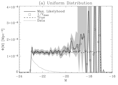
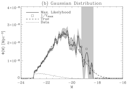
Figure 13.— Numerical tests to our maximum likelyhood LF estimate. The various types of lines and symbols correspond to the true LF (the dashed line), the restored $1/V_{\rm max}$ LF (square symbols), and the maximum likelyhood LF (the solid line, with the shaded region representing the error bars). The dotted line corresponds to the original data offered to the LF retrieval routine. (a) Case where the true LF is a uniform distribution between magnitudes -23 and -17. (b) Same as (a) except that the underlying LF is a truncated Gaussian.

References

- Adelman-McCarthy & the SDSS collaboration (2007) Adelman-McCarthy, J. K. & the SDSS collaboration. 2007, AJ, astro-ph/07073413v2
- Allam et al. (2005) Allam, S. S., Tucker, D. L., Lee, B. C., & Smith, J. A. 2005, AJ, 129, 2062
- Aloisi et al. (2007) Aloisi, A., Clementini, G., Tosi, M., et al. 2007, ApJ, 667, L151
- Amorín et al. (2008) Amorín, R. O., Aguerri, J. A. L., Muñoz-Tuñón, C., & Cairós, L. M. 2008, A&A, submitted
- Amorín et al. (2007) Amorín, R. O., Muñoz-Tuñón, C., Aguerri, J. A. L., Cairós, L. M., & Caon, N. 2007, A&A, 467, 541
- Balogh et al. (2004) Balogh, M. L., Baldry, I. K., Nichol, R., et al. 2004, ApJ, 615, L101
- Beltrametti et al. (1982) Beltrametti, M., Tenorio-Tagle, G., & Yorke, H. W. 1982, A&A, 112, 1
- Bergvall & Östlin (2002) Bergvall, N. & Östlin, G. 2002, A&A, 390, 891
- Bershady et al. (2000) Bershady, M. A., Jangren, A., & Conselice, C. J. 2000, AJ, 119, 2645
- Blanton et al. (2001) Blanton, M. R., Dalcanton, J., Eisenstein, D., et al. 2001, AJ, 121, 2358
- Blanton et al. (2003a) Blanton, M. R., Hogg, D. W., Bahcall, N. A., et al. 2003a, ApJ, 594, 186
- Blanton et al. (2003b) Blanton, M. R., Hogg, D. W., Bahcall, N. A., et al. 2003b, ApJ, 592, 819
- Blanton et al. (2005) Blanton, M. R., Lupton, R. H., Schlegel, D. J., et al. 2005, ApJ, 631, 208
- Bolzonella et al. (2002) Bolzonella, M., Pelló, R., & Maccagni, D. 2002, A&A, 395, 443
- Cairós et al. (2003) Cairós, L. M., Caon, N., Papaderos, P., et al. 2003, ApJ, 593, 312
- Cairós et al. (2001) Cairós, L. M., Caon, N., Vílchez, J. M., González-Pérez, J. N., & Muñoz-Tuñón, C. 2001, ApJS, 136, 393
- Caon et al. (2005) Caon, N., Cairós, L. M., Aguerri, J. A. L., & Muñoz-Tuñón, C. 2005, ApJS, 157, 218
- Ciotti (1991) Ciotti, L. 1991, A&A, 249, 99
- Corbin et al. (2007) Corbin, M. R., Kim, H., Jansen, R. A., Windhorst, R. A., & Cid Fernandes, R. 2007, ApJ, in press, astroph/0710.2557
- Dalcanton (2007) Dalcanton, J. J. 2007, ApJ, 658, 941
- Davies & Phillipps (1988) Davies, J. I. & Phillipps, S. 1988, MNRAS, 233, 553
- Davis & Huchra (1982) Davis, M. & Huchra, J. 1982, ApJ, 254, 437
- Diemand et al. (2007) Diemand, J., Kuhlen, M., & Madau, P. 2007, ApJ, 657, 262
- Efstathiou et al. (1988) Efstathiou, G., Ellis, R. S., & Peterson, B. A. 1988, MNRAS, 232, 431
- Fukugita et al. (1996) Fukugita, M., Ichikawa, T., Gunn, J. E., et al. 1996, AJ, 111, 1748
- Gil de Paz & Madore (2005) Gil de Paz, A. & Madore, B. F. 2005, ApJS, 156, 345
- Gil de Paz et al. (2003) Gil de Paz, A., Madore, B. F., & Pevunova, O. 2003, ApJS, 147, 29
- Graham et al. (2005) Graham, A. W., Driver, S. P., Petrosian, V., et al. 2005, AJ, 130, 1535
- Graham & Guzmán (2003) Graham, A. W. & Guzmán, R. 2003, AJ, 125, 2936
- Heavens et al. (2004) Heavens, A., Panter, B., Jimenez, R., & Dunlop, J. 2004, Nature, 428, 625
- Heckman (2002) Heckman, T. M. 2002, in ASP Conf. Ser., Vol. 254, Extragalactic Gas at Low Redshift, ed. J. S. Mulchaey & J. Stocke (San Francisco: ASP), 292
- Kauffmann et al. (2003) Kauffmann, G., Heckman, T. M., Tremonti, C., et al. 2003, MNRAS, 346, 1055
- Kazantzidis et al. (2007) Kazantzidis, S., Bullock, J. S., Zentner, A. R., Kravtsov, A. V., & Moustakas, L. A. 2007, ApJ, submitted, astro-ph/07081949
- Kennicutt (1998) Kennicutt, R. C. 1998, ARA&A, 36, 189
- Kunth & Östlin (2000) Kunth, D. & Östlin, G. 2000, A&A Rev., 10, 1
- Legrand et al. (2001) Legrand, F., ; Tenorio-Tagle, G., Silich, S., Kunth, D., & Cerviño, M. 2001, ApJ, 560, 630
- Leonardi & Rose (1996) Leonardi, A. J. & Rose, J. A. 1996, AJ, 111, 182
- Leonardi & Worthey (2000) Leonardi, A. J. & Worthey, G. 2000, ApJ, 534, 650
- Lilly et al. (1996) Lilly, S. J., Le Fevre, O., Hammer, F., & Crampton, D. 1996, ApJ, 460, L1
- Lin et al. (1996) Lin, H., Kirshner, R. P., Shectman, S. A., et al. 1996, ApJ, 471, 617
- Madau et al. (1996) Madau, P., Ferguson, H. C., Dickinson, M. E., et al. 1996, MNRAS, 283, 1388
- Malmberg (2005) Malmberg, D. 2005, Master’s thesis, Uppsala University, Uppsala
- Marlowe et al. (1999) Marlowe, A. T., Meurer, G. R., & Heckman, T. M. 1999, ApJ, 522, 183
- Martin (1971) Martin, B. R. 1971, Statistics for Physicists (London: Academic Press)
- Mas-Hesse & Kunth (1999) Mas-Hesse, J. M. & Kunth, D. 1999, A&A, 349, 765
- Moore et al. (2003) Moore, D. S., McCabe, G. P., Duckworth, W. M., & Sclove, S. L. 2003, The practice of business statistics: using data for decisions (New York: W. H. Freeman and Co)
- Pagel & Edmunds (1981) Pagel, B. E. J. & Edmunds, M. G. 1981, ARA&A, 19, 77
- Papaderos et al. (1996a) Papaderos, P., Loose, H.-H., Fricke, K. J., & Thuan, T. X. 1996a, A&A, 314, 59
- Papaderos et al. (1996b) Papaderos, P., Loose, H.-H., Thuan, T. X., & Fricke, K. J. 1996b, A&AS, 120, 207
- Pilyugin et al. (2004) Pilyugin, L. S., Vílchez, J. M., & Contini, T. 2004, A&A, 425, 849
- Press et al. (1988) Press, W. H., Flannery, B. P., Teukolsky, S. A., & Vetterling, W. T. 1988, Numerical Recipes (Cambridge: Cambridge University Press)
- Sage et al. (1992) Sage, L. J., Salzer, J. J., Loose, H.-H., & Henkel, C. 1992, A&A, 265, 19
- Sargent & Searle (1970) Sargent, W. L. W. & Searle, L. 1970, ApJ, 162, L155
- Schlegel et al. (1998) Schlegel, D. J., Finkbeiner, D. P., & Davis, M. 1998, ApJ, 500, 525
- Schmidt (1959) Schmidt, M. 1959, ApJ, 129, 243
- Schmidt (1968) Schmidt, M. 1968, ApJ, 151, 393
- Searle & Sargent (1972) Searle, L. & Sargent, W. L. W. 1972, ApJ, 173, 25
- Searle et al. (1973) Searle, L., Sargent, W. L. W., & Bagnuolo, W. G. 1973, ApJ, 179, 427
- Shi et al. (2005) Shi, F., Kong, X., Li, C., & Cheng, F. Z. 2005, A&A, 437, 849
- Silich & Tenonio-Tagle (2001) Silich, S. & Tenonio-Tagle, G. 2001, ApJ, 552, 91
- Silk et al. (1987) Silk, J., Wyse, R. F. G., & Shields, G. A. 1987, ApJ, 322, L59
- Skillman et al. (1989) Skillman, E. D., Kennicutt, R. C., & Hodge, P. W. 1989, ApJ, 347, 875
- Smith et al. (2002) Smith, J. A., Tucker, D. L., Kent, S., et al. 2002, AJ, 123, 2121
- Staveley-Smith et al. (1992) Staveley-Smith, L., Davies, R. D., & Kinnan, T. D. 1992, MNRAS, 258, 334
- Stoughton et al. (2002) Stoughton, C., Lupton, R. H., Bernardi, M., et al. 2002, AJ, 123, 485
- Takeuchi et al. (2000) Takeuchi, T. T., Yoshikawa, K., & Ishii, T. T. 2000, ApJS, 129, 1
- Telles & Terlevich (1997) Telles, E. & Terlevich, R. 1997, MNRAS, 286, 183
- Tenorio-Tagle et al. (2003) Tenorio-Tagle, G., Silich, S., & Muñoz-Tuñón, C. 2003, ApJ, 597, 279
- Tenorio-Tagle et al. (2005) Tenorio-Tagle, G., Silich, S., Rodríguez-González, A., & Muñoz-Tuñón, C. 2005, ApJ, 628, L13
- Terlevich et al. (1990) Terlevich, E., Diaz, A. I., & Terlevich, R. 1990, MNRAS, 242, 271
- Terlevich et al. (1991) Terlevich, R., Melnick, J., Masegosa, J., Moles, M., & Copetti, M. V. F. 1991, A&AS, 91, 285
- Thuan (1991) Thuan, T. X. 1991, in Massive Stars in Starbursts, ed. C. Leitherer, N. Walborn, T. Heckman, & C. Norman (Cambridge: Cambridge University Press), 183
- Tinsley (1980) Tinsley, B. M. 1980, Fundam. Cosmic Phys., 5, 287
- Wakker et al. (2007) Wakker, B. P., York, D. G., Howk, J. C., et al. 2007, ApJ, 670, L113
- Worthey et al. (1994) Worthey, G., Faber, S. M., Gonzalez, J. J., & Burstein, D. 1994, ApJS, 94, 687
- Zackrisson et al. (2006) Zackrisson, E., Bergvall, N., Östlin, G., Micheva, G., & Leksell, M. 2006, ApJ, 650, 812