IPPP/08/21 DCPT/08/42

Electroweak Precision Data
and the Lee-Wick Standard Model
Thomas E. J. Underwood¹ and Roman Zwicky^{2 1} Max-Planck-Institut für Kernphysik, Saupfercheckweg 1, 69117 Heidelberg, Germany ² IPPP, Department of Physics, Durham University, Durham DH1 3LE, UK

Abstract:
We investigate the electroweak precision constraints on the recently proposed Lee-Wick Standard Model at tree level. We analyze low energy, Z-pole (LEP1/SLC) and LEP2 data separately. We derive the exact tree level low energy and Z-pole effective Lagrangians from both the auxiliary field and higher derivative formulation of the theory. For the LEP2 data we use the fact that the Lee-Wick Standard Model belongs to the class of models that assumes a so-called‘universal’ form which can be described by seven oblique parameters at leading order in $m_{W}^{2}/M_{1,2}^{2}$. At tree level we find that $Y=-m_{W}^{2}/M_{1}^{2}$ and $W=-m_{W}^{2}/M_{2}^{2}$, where the negative sign is due to the presence of the negative norm states. All other oblique parameters $(\hat{S},X)$ and $(\hat{T},\hat{U},V)$ are found to be zero. In a separate addendum we show how our results differ from previous investigations, where contact terms, which are found to be of leading order, have been neglected. The LEP1/SLC constraints are slightly stronger than LEP2 and much stronger than the low energy ones. The LEP1/SLC results exclude gauge boson masses of $M_{1}\simeq M_{2}\sim 3\,{\rm TeV}$ at the $99\%$ confidence level. Somewhat lower masses are possible when one of the masses assumes a large value. Loop corrections to the electroweak observables are suppressed by the standard $\sim 1/(4\pi)^{2}$ factor and are therefore not expected to change the constraints on $M1$ and $M_{2}$. This assertion is most transparent from the higher derivative formulation of the theory.

1 Introduction

In 1970 Lee and Wick (LW) proposed a finite theory of QED [1, 2]. Just over a year ago, Grinstein, O’Connell and Wise (GOW) [3] extended those ideas to non-Abelian gauge theories and chiral fermions and constructed a Lee-Wick Standard Model (LWSM). The essence of the work by LW was to introduce Pauli-Villars, wrong-sign propagator, fields as physical degrees of freedom. Since the interaction terms only contain certain combinations of fields and ghost fields, the latter can be integrated out at the cost of introducing higher derivative (HD) interactions. The new degrees of freedom lead to amplitudes which are better behaved in the ultraviolet and render the logarithmically divergent QED finite. It was shown by GOW [3] that the LWSM is free from quadratic divergences and therefore provides a possible solution to the ‘hierarchy problem’. It was also shown that the addition of very heavy right handed neutrinos, in the context of the see-saw mechanism, does not destabilize the Higgs mass [4].

The introduction of the Pauli-Villars wrong sign states brings into question basic concepts such as causality and unitarity. These issues were investigated in some detail in the 1970’s and some results are summarized in the Erice Lectures of Lee [5] and Coleman [6]. In reference [6] it is illustrated that the wrong sign of the width compensates for the wrong sign in the propagator to ensure unitarity in a simple s-channel process. The wrong sign of the width in turn implies that poles will move into the physical sheet which demands a new contour prescription [7]. The modification of the contour might bring into question Lorentz invariance, c.f. references [8] for criticism and [9] for a response. In summary, the current status is that there are no known examples in perturbation theory which are in conflict with unitarity when applying the contour modification of [7] and acausal phenomena arises only at scales which are not accessible to current experiments. The phenomenon of causality was reconsidered only very recently in an $O(N)$ model [10]. The authors investigate the large N limit, where the theory is described by a single one-loop bubble, and obtain a unitary and Lorentz invariant scattering amplitude. Furthermore, a non-perturbative definition through the path integral via the contour deformation [7] does not seem to be straightforward or conclusive [11]. A higher derivative version of the LW Higgs sector was used for lattice field theory [12, 13]. This is of great interest because it can smooth cut-off dependences. As stated in reference [12] this does not really clarify the issue in Minkowski space since an analytic continuation is prevented by the complex ghost poles. A path integral approach with test functions was recently proposed [14], from where the contour prescription can be derived.

Following the proposal of the LWSM several phenomenological investigations have been pursued. The low Higgs mass discovery channel $gg\to h_{0}\to\gamma\gamma$ was found to be moderately positively enhanced, $5$-$20\%$ for the top LW at $0.5$-$1\,{\rm TeV}$ [18]. It is a curious fact, or a rather unique signature of the ghost fields, that the CKM elements $|V_{\rm tx}|$ are accompanied by an enhancement factor $(1+(m_{t}/M_{\rm LW})^{2}/2)$ which can lead to $|V_{\rm tx}|\gtrsim 1$ at the few percent level [18]. Flavour changing neutral currents induced by integrating out heavy LW fermions have been found to give acceptably small contributions for a LW mass scale $M_{\rm LW}\sim 1\,{\rm TeV}\cite[cite]{[\@@bibref{}{DW}{}{}]}$. LW gauge bosons were found to lead to possible signatures of a unique nature both at the LHC in dijet channels [16] and in cross-sections and left-right asymmetries in Bhabba scattering at linear colliders [17].

Aspects of LW gauge theories unrelated to the LWSM have also found attention. The running of a non-Abelian LW theory coupled to a scalar field was investigated in [19], where it was found that the gauge coupling runs faster than in an ordinary gauge theory. It was also shown that massive LW gauge bosons do not require a Higgs degree of freedom to unitarize amplitudes at high energy [20]. This is because the formulation is gauge invariant without a Higgs field and corresponding Ward identities assure a moderate growth at high energy. Abelian and non-Abelian LW gauge theories have also been to shown to give rise to chiral symmetry breaking [21]. Moreover it has been suggested that gravitational 1-loop corrections may lead to the appearance of a Lee-Wick photon [22]. This effect has recently also been studied in the context of large extra dimensions [23].

In this paper we analyse the constraints on the LWSM gauge boson sector coming from low energy, $Z$-pole and LEP-2 data. We will work at tree level, an approximation justified as we do not see any reason for loop corrections to compete with tree level contributions relieving the $\sim 1/(4\pi)^{2}$ hierarchy. Even though we find that among the three symmetry classes of the oblique parameters two are vanishing at tree level, it is not necessary to calculate the loop contributions to those parameters as the seven oblique parameters all have similar experimental constraints and are typically of the same order when no symmetry is protecting them. Possibly an exception to this rule is the breaking of custodial symmetry at loop level due to the mass splitting of the third family. This contributes to the rho parameter as $\Delta\rho_{*}(0)=\alpha T=\hat{T}$. It is well known that the dominant correction to the rho parameter in the SM is due to fermion loops and is given by $\Delta\rho_{*}(0)^{\rm SM}\simeq G_{F}m_{t}^{2}/(8\pi^{2}\sqrt{2})\simeq 10^{-2}$ e.g. [36]. An easy way to obtain a crude estimate of this contribution in LWSM is to take a look at the HD formulation,

$$\hat{\Delta}(p)=\frac{1}{p^{2}-p^{4}/M_{\rm LW}^{2}-m^{2}}\,,\qquad\hat{S}_{F}(p)=\frac{\hbox to0.0pt{\kern 0.50314pt/\hss}p\big{(}1-\frac{p^{2}}{M_{\rm LW}^{2}}\big{)}+m}{p^{2}(1-\frac{p^{2}}{M_{\rm LW}^{2}}\big{)}^{2}-m^{2}}\,.$$ (1)

indicating a contribution to the rho parameter $|\Delta\rho_{*}(0)^{\rm LWSM}|\sim{\cal O}(1)\,10^{-2}(m_{t}/M_{\rm LW})^{2}$, up to further logarithmic corrections. From the constraint $|\Delta\rho_{*}(0)|<10^{-3}$ [25] one could then deduce limits on $m_{\tilde{t}}$.

We feel obliged to comment on other papers that have investigated electroweak precision constraints on the LWSM [24, 41]. Our results differ conceptually from theirs by including effects of contact terms. The latter are found to be of leading order and are therefore necessary ingredient to a consistent analysis. Further details about this relation can be found in a separate addendum to this paper. We would like to mention that our results for the oblique parameters, which rely on an expansion in $m_{W,Z}^{2}/M_{\rm new}^{2}$ are backed-up by an exact treatment of the tree level low-energy and $Z$-pole Lagrangians. Further comments and more details on the origin of these discrepancies can be found in an addendum at the end of this paper.

We would also like to make some comments on observables which we have omitted in this paper. For instance one of the LWSM contributions to the anomalous magnetic moment of the muon, $(g-2)_{\mu}$ is given by Schwinger’s vertex correction where the photon is replaced by the Lee-Wick photon. The form of the propagators in the LWSM suggests that this contribution is suppressed with respect to the corresponding SM contribution by a factor $(m_{\mu}/M_{1})^{2}\sim 10^{-8}$, with $M_{1}\sim 1\,{\rm TeV}$ according to the high energy constraints investigated in this paper. This value is about two orders of magnitude too low to explain the difference between theory and experiment. Notice that the situation is rather different to the MSSM, for example, because the contraints on the scale analogous to $M_{1}$ are not so tight there since tree level constraints from other precision data are absent. The MSSM contribution is also sensitive to enhancements by factors of $\tan\beta$. The contributions to the rate for $b\to s\gamma$ would be interesting to study. The dominant contribution is due to penguins with top loops and we would therefore expect to either obtain constraints on the LW fermion mass scale or better agreement between experiment and theory.

We refrain from reviewing the LWSM itself in more detail and refer instead to the original paper [3] and our own paper in connection with the matrix notation for the LW generations [18]. The paper is organized as follows. In section 2 we analyse the electroweak sector of the LWSM. We derive the low energy effective Lagrangian at tree level in the auxiliary field and the HD formulation in subsection 2.1. The effective Lagrangian relevant to data collected at the $Z$-pole is derived in section 2.2 in both formalisms. The LEP-2 data is assessed via the oblique approximation in section 2.3, where we also rederive the results of the previous section in the oblique approximation. In section 3 we relate the parameters of the effective Lagrangian to the observables and detail the sources of our experimental input and procedures. Concluding remarks can be found in section 4.

Details of the gauge boson propagators in the higher derivative formalism are given in appendix A. Some exact results for diagonalization of the gauge boson mass matrices, for the case where the SU(2)_L and U(1)_Y LW extensions are degenerate in their mass scale $M_{1}=M_{2}$, are given in appendix B.

Throughout the paper we neglect terms of the order of $m_{f}m_{f}^{\prime}/M_{\rm LW}^{2}$, where the $f$ is any fermion other than the top quark. In particular, this implies that we are allowed to omit contributions from longitudinal components of gauge bosons ${\cal O}(p_{\mu}p_{\nu})$ and neglect diagonalization of mass matrices in the fermion sector (although this was outlined in [18]).

2 Effective Lagrangians for electroweak constraints

The low energy effective Lagrangian, Z-pole observables and the constraints from LEP-2 are investigated in sections 2.1, 2.2, 2.3 respectively. The low energy Lagrangian is rather straightforward whereas the exact Z-pole effective Lagrangian demands the diagonalization of the Z-boson sector. In the LEP-2 section we will exploit the fact that the LWSM belongs to the class of “universal” Lagrangians which allow the parameterization of the leading electroweak corrections in terms of seven oblique parameters $(S,T,U,V,W,X,Y)$. By leading we mean to first order in $m_{W}^{2}/M^{2}$ where $M$ is the mass scale of the LW gauge bosons. We will rederive all the results of the previous sections in this approximation. The reader who is familiar with electroweak precision data and the formalisms used to constrain it can directly go to section 2.3 with the additional information that among the three best measured parameters [25],

$${{m}_{Z,\rm ph}} = 91.1876(21)\,{\rm GeV}\,,$$

$$\alpha({{m}_{Z,\rm ph}}) = \frac{1}{127.918(18)}\,,$$

$$G_{F} = 1.16637(1)\cdot 10^{-5}\,{\rm GeV^{2}}\,,$$ (2)

only ${{m}_{Z,\rm ph}}$ receives corrections. This implies a correction to the Weinberg angle.

2.1 Low energy effective Lagrangian

The low energy effective electroweak Lagrangian can be parametrised as

$${\cal L}^{\rm eff}_{\rm EW}=-\frac{4G_{F}}{\sqrt{2}}\Big{(}J_{+}\!\cdot\!J_{-}+\rho_{*}(0)J_{\rm nc}^{2}\Big{)}+C_{Q}J_{Q}^{2}\,,$$ (3)

with

$$J_{\pm}^{\mu}=(J_{1}\pm iJ_{2})^{\mu}\,,\qquad J_{\rm nc}^{\mu}\equiv(J_{3}-s^{2}_{*}(0)J_{Q})^{\mu}\,.$$ (4)

in terms of four parameters

$$p_{\rm low}\equiv[\rho_{*}(0),s^{2}_{*}(0),G_{F},C_{Q}]\,,$$ (5)

which assume the values

$$(p_{\rm low})_{SM}=[1,\sin(\theta_{W})^{2},\frac{1}{\sqrt{2}v^{2}},0]\,,$$ (6)

in the SM. In the following two subsections we will derive the values of the four low energy parameters in the LWSM using both the auxiliary field and the higher derivative (HD) formalisms.

2.1.1 Auxiliary field formalism

The low energy effective Lagrangian can be derived in the auxilliary field picture by integrating out the heavy gauge degrees of freedom (i.e. all gauge fields except for the photon). To do this in an efficient manner the matrix formalism introduced in reference [18] is extended to the gauge boson current sector,

$${\cal L}_{\rm EW}=-{\cal J}^{{\rm a}\,\top}\!\cdot\!{\cal W}^{{\rm a}\,}-{\cal J}^{0\,\top}\!\cdot\!{\cal B}+\frac{1}{2}\,{\cal W}^{{\rm a}\,\mu\,\top}{\cal M}_{\cal W}\,\eta_{2}\,{\cal W}^{{\rm a}}_{\mu}+\frac{1}{2}\,{\cal B}^{\mu\,\top}{\cal M}_{\cal B}\,\eta_{4}\,{\cal B}_{\mu}+\ldots\,,$$ (7)

with

$${\cal J}^{{\rm a}\,\top}_{\mu} =g_{2}\big{(}J,\,J\big{)}^{\rm a}_{\mu}\,,\qquad {\cal J}^{0\,\top}_{\mu}= \,\,\big{(}g_{1}J^{Y},\,g_{2}J^{3},\,g_{1}J^{Y},\,g_{2}J^{3}\big{)}_{\mu}\,,$$

$${\cal W}_{\mu}^{{\rm a}\,\top} =\big{(}W,\,\widetilde{W}\big{)}^{\rm a}_{\mu}\,, {\cal B}_{\mu}^{\top}= \,\,\big{(}B,\,W^{3},\,\tilde{B},\,\widetilde{W}^{3}\big{)}_{\mu}\,,$$ (8)

where $J^{\rm a}_{\mu}$ and $J^{Y}_{\mu}$ are the appropriate fermion currents, ${\cal M}_{\cal B}$ and ${\cal M}_{\cal W}$ are the neutral and charged gauge boson mass matrices, $\eta_{2}={\rm diag}(1,-1)$, $\eta_{4}={\rm diag}(1,1,-1,-1)$ and ${\rm a}=\{1,2\}$. The dots refer to cubic and quartic couplings between the gauge bosons. For ${\cal M}_{\cal B}$ and ${\cal M}_{\cal W}$ we have

$${\cal M}_{\cal B}\,\eta_{4} = \left(\begin{array}[]{lc}M_{\rm SM}&M_{\rm SM}\\ M_{\rm SM}&M_{\rm SM}-M_{12}\end{array}\right)\,,\quad M_{\rm SM}\ =\ \frac{v^{2}}{4}\left(\begin{array}[]{cc}g_{1}^{2}&-g_{1}\,g_{2}\\ -g_{1}\,g_{2}&g_{2}^{2}\end{array}\right)\,,$$ (13)

$${\cal M}_{\cal W}\,\eta_{2} = \frac{1}{4}\left(\begin{array}[]{cc}g_{2}^{2}\,v^{2}&g_{2}^{2}\,v^{2}\\ g_{2}^{2}\,v^{2}&g_{2}^{2}\,v^{2}-4M_{2}^{2}\end{array}\right)\,,\quad M_{12}\ =\ \left(\begin{array}[]{cc}M_{1}^{2}&0\\ 0&M_{2}^{2}\end{array}\right)\,.$$ (18)

The charged current sector is straightforward. Integrating out the charged gauge bosons at tree level is equivalent to applying the equation of motions (eom)

$${\cal W}^{\rm a}_{\mu}=\big{(}{\cal M}_{\cal W}\,\eta_{2}\big{)}^{-1}\,{\cal J}^{\rm a}_{\mu}\,,$$ (19)

for the ${\cal W}^{\rm a}_{\mu}$ fields.

The neutral sector is more involved because the massless photon has to be decoupled in order to invert the mass matrix. This is easily done using the transformation ${\cal B}\to S\,{\cal B}^{\prime}$ where $S\,\eta_{4}\,S^{\dagger}\,\eta_{4}=\mathbb{I}$ and

$$S=\left(\begin{array}[]{cc}R_{W}&0_{2}\\ 0_{2}&\mathbb{I}_{2}\end{array}\right)\qquad{\rm with}\qquad R_{W}=\left(\begin{array}[]{cc}c&-s\\ s&c\end{array}\right)\,,$$ (20)

and

$$s\equiv\sin\theta_{W}\,,\qquad c\equiv\cos\theta_{W}\,,\qquad t\equiv\tan\theta_{W}\equiv g_{1}/g_{2}\,.$$ (21)

It is straightforward to verify that $S^{\top}\,{\cal M}_{\cal B}\eta_{4}\,S$ is block-diagonal with one zero eigenvalue.

Denoting the projection of the primed currents and mass matrices on the heavy gauge boson subspace by a double prime, the neutral gauge boson Lagrangian reads

$${\cal L}=-{\cal J}^{0\prime\prime\,\,\top}\!\cdot\!{\cal B}^{\prime\prime}+\frac{1}{2}\,{\cal B}^{\prime\prime\,\mu\,\top}{\cal M}^{\prime\prime}_{\cal B}\,\eta_{3}\,{\cal B}^{\prime\prime}_{\mu}\,\,-e\,A\!\cdot\!J^{Q}\,,$$ (22)

where $e\equiv g_{2}s$,

$${\cal B}^{\prime\prime\top}_{\mu}=\big{(}cW^{3}-sB,\tilde{B},\widetilde{W}^{3}\big{)}_{\mu}\,,\qquad{\cal J}^{0\prime\prime\top}_{\mu}=e\left(\frac{c}{s}J^{3}-\frac{s}{c}J^{Y},\frac{1}{c}J^{Y},\frac{1}{s}J^{3}\right)_{\mu}\,,$$ (23)

and

$${\cal M}^{\prime\prime}_{\cal B}\,\eta_{3}=m_{Z}^{2}\,\left(\begin{array}[]{ccc}1&-s&c\\ -s&\;\;\;s^{2}-x_{1}&-s\,c\\ c&-s\,c&c^{2}-x_{2}\end{array}\right)\,,$$ (24)

where $\eta_{3}={\rm diag}(1,-1,-1)$ and

$$x_{i}\equiv\frac{M_{i}^{2}}{m_{Z}^{2}}\,,\qquad m_{Z}^{2}\equiv\frac{e^{2}v^{2}}{4s^{2}c^{2}}\,,$$ (25)

are notations frequently used throughout the paper.

The massive neutral gauge bosons may be integrated out by substituting the following expression obtained from the eom for ${\cal B}^{\prime\prime}_{\mu}$ into Eq. (22), i.e.

$${\cal B}^{\prime\prime}_{\mu}=\big{(}{\cal M}_{\cal B}^{\prime\prime}\,\eta_{3}\big{)}^{-1}{\cal J}^{0\prime\prime}_{\mu}\,.$$ (26)

After some algebra, the electroweak low-energy effective Lagrangian can now be written down

$${\cal L}^{\rm eff}_{\rm EW}=-\ eA\!\cdot\!J^{Q}\ -\ \frac{2}{v^{2}}\Big{(}J_{+}\!\cdot\!J_{-}\ +\ \big{(}J_{3}-s^{2}J_{Q}\big{)}^{2}\Big{)}\ +\ \frac{e^{2}}{2}\Big{(}\frac{c^{2}}{M_{1}^{2}}+\frac{s^{2}}{M_{2}^{2}}\Big{)}J_{Q}^{2}\,.$$ (27)

By comparing Eq. (27) with Eq. (3) we can read off expressions for the the Fermi constant $G_{F}$ and the parameters $\rho_{*}(0)$, $s^{2}_{*}(0)$ and $C_{Q}$

$$G_{F}=\frac{1}{\sqrt{2}\,v^{2}}\,,\quad\rho_{*}(0)=1\,,\quad\quad s^{2}_{*}(0)=s^{2}\,,\quad C_{Q}=\frac{e^{2}}{2}\Big{(}\frac{c^{2}}{M_{1}^{2}}+\frac{s^{2}}{M_{2}^{2}}\Big{)}\,.$$ (28)

Note that the electromagnetic coupling $4\pi\alpha=e^{2}$ is not affected since the photon cannot be integrated out. The coefficient $C_{Q}$ cannot be seen at low energies anticipating the LW gauge boson masses to be around $M_{i}\sim 1\,{\rm TeV}$, because it is shielded by the photon background by a very small factor $s_{\rm c.m.}/M_{i}^{2}$. The scale $s_{\rm c.m.}$ refers to data points in $e^{+}e^{-}\to{\rm hadrons}$ [25] and $s_{\rm c.m.}\ll m_{Z}^{2}$ as otherwise the effective description breaks down. The $C_{Q}$ term corresponds to a contact term originating from the massive LW photon. We already want to point out at this stage that the low energy observables will receive corrections through $s$ due to a shift in ${{m}_{Z,\rm ph}}$, which we will derive in the next chapter.

2.1.2 Higher derivative formalism

In order to derive the low energy effective Lagrangian in the higher derivative picture we need the $W$ and $Z$ propagators in this formalism. The coupling of the gauge bosons is identical to the SM, up to corrections of the type $\partial^{2}/M_{LW}^{2}$, which are irrelevant at low energy. The SM gauge boson current Lagrangian is given by

$${\cal L}=-\frac{g_{2}}{\sqrt{2}}(W^{+}\!\cdot\!J^{+}+W^{-}\!\cdot\!J^{-})-\frac{g_{2}}{c}Z\!\cdot\!J_{\rm nc}-eA\!\cdot\!J_{Q}\,,$$ (29)

where $W^{\pm}=(W^{1}\pm iW^{2})/\sqrt{2}$ and the currents have been defined in Eq. (4). It is rather straightforward to show that the HD propagator assumes the following form

$$\hat{D}^{W}_{\mu\nu}(p^{2})=\hat{D}^{W}(p^{2})\Big{(}-g_{\mu\nu}+p_{\mu}p_{\nu}f^{W}_{pp}\Big{)}\,,\quad\quad D^{W}(p^{2})=\frac{i}{p^{2}-m_{W}^{2}-p^{4}/M_{2}^{2}},$$ (30)

with

$$m_{W}^{2}\equiv\frac{e^{2}v^{2}}{4s^{2}}\,,$$ (31)

in analogy with the definitions (25). More details and an explicit expression for $f_{pp}^{W}$ are given in appendix A. The charged low energy effective action follows then from Eq. (29)

$${\cal L}^{\rm eff}_{\rm CC}=-i\hat{D}^{W}(0)\frac{g_{2}^{2}}{2}J_{+}\!\cdot\!J_{-}=-\frac{g_{2}^{2}}{2m_{W}^{2}}J_{+}\!\cdot\!J_{-}\,.$$ (32)

The propagator of the neutral gauge bosons $\hat{N}=(\hat{Z},\hat{A})$ has the form

$$\hat{D}_{\mu\nu}^{N}(p^{2})=\hat{D}^{N}(p^{2})(-g_{\mu\nu}+p_{\mu}p_{\nu}f^{N}_{pp})\,.$$ (33)

This propagator is non-diagonal in the $(\hat{Z},\hat{A})$ space if $M_{1}\neq M_{2}$. Further details can be found in appendix A Eq. (A) The neutral low energy effective Lagrangian is given by

$${\cal L}_{\rm NC}^{\rm eff} = -i\frac{g_{2}^{2}}{2c^{2}}\Big{(}J_{N}^{\mu\,\,T}(\hat{D}^{N}(p^{2})-\left(\begin{array}[]{cc}0&0\\ 0&1\end{array}\right)\frac{i}{p^{2}})J_{N}^{\mu}\Big{)}_{p^{2}\to 0}\,,$$ (36)

$$= -\frac{g_{2}^{2}}{2m_{W}^{2}}J_{Z}^{2}+\frac{e^{2}}{2}\Big{(}\frac{c^{2}}{M_{1}^{2}}+\frac{s^{2}}{M_{2}^{2}}\Big{)}J_{Q}^{2}\,,$$ (37)

with the photon pole subtracted since the photon cannot be integrated out. We have implicitly used the notation $J_{N}=(\frac{g_{2}}{c}J_{Z},eJ_{Q})$. From the low energy effective interactions (32) and (36) and the parametrisation (3) and (4) we read off the same parameters as in Eq. (28).

2.2 Effective Lagrangian at the Z-pole

When considering experimental data collected at LEP and SLC around the $Z$-pole, generic “new physics” can be parameterised by the Lagrangian

$${\cal L}={\cal L}^{SM}(e,s,v)+\delta{\cal L}^{\rm new}(e,s,v,..)\,.$$ (38)

However, the parameters fitted to experimental data are not the ($e,s,v$) but other parameters ($e_{0},s_{0},v_{0}$), which are defined using the three best measured observables $\alpha$, $G_{F}$ and ${{m}_{Z,\rm ph}}$ mentioned at the beginning of this section. These may be written

$$m_{Z,0}^{2} \equiv{{m}^{2}_{Z,\rm ph}}=m_{Z}^{2}(1+\delta_{Z})\qquad\qquad\qquad m_{Z}=\frac{ev}{2cs}$$

$$\alpha_{0}({{m}_{Z,\rm ph}}) \equiv\alpha({{m}_{Z,\rm ph}})=\alpha({{m}_{Z,\rm ph}})_{SM}(1+\delta_{\alpha}) \alpha({{m}_{Z,\rm ph}})_{SM}=\frac{e^{2}}{4\pi}$$

$$G_{F,0} \equiv G_{F}=(G_{F})_{SM}(1+\delta_{G}) (G_{F})_{SM}=\frac{1}{\sqrt{2}v^{2}}$$ (39)

Using the measured values of $G_{F}$, $\alpha$ and ${{m}_{Z,\rm ph}}$ we can obtain the following three fundamental parameters of the SM Lagrangian

$$e=\sqrt{\frac{4\pi\alpha({{m}_{Z,\rm ph}})}{1+\delta_{\alpha}}}\,,\qquad v=\sqrt{\frac{(1+\delta_{G})}{\sqrt{2}G_{F}}}\,,$$

$$s^{2}c^{2}=s_{0}^{2}c_{0}^{2}\frac{(1+\delta_{G})(1+\delta_{Z})}{1+\delta_{\alpha}}\,,$$ (40)

with the well-measured intermediate quantity $s_{0}$ defined as

$$\frac{1}{4}\sin^{2}(2\theta_{0})=s_{0}^{2}c_{0}^{2}\equiv\frac{\pi\alpha({{m}_{Z,\rm ph}})}{\sqrt{2}G_{F}M_{Z}^{2}}\,,$$ (41)

with $s_{0}=\sin(\theta_{0})$ and $c_{0}=\cos(\theta_{0})$. As mentioned in the introduction, the low energy observables will receive corrections due to the non-trivial relation between $(s,c)$ and $(s_{0},c_{0})$ given in Eq. (2.2).

It is convenient to parameterise couplings of the $Z$ to fermions in terms of the following generalised Lagrangian [29]

$${\cal L}_{Z}^{\rm eff}=-\,\frac{e_{0}}{s_{0}c_{0}}\sum_{i}\bar{f}_{i}\gamma^{\mu}\Big{[}\big{(}g^{f,SM}_{L}+\delta g^{f}_{L}\big{)}P_{L}+\big{(}g^{f,SM}_{R}+\delta g^{f}_{R}\big{)}P_{R}\Big{]}f_{i}\,Z_{\mu}\,,$$ (42)

where $P_{L,R}$ are the usual left and right projection operators and

$$g^{f,SM}_{L}=t_{3}^{f}-q^{f}s_{0}^{2}\,,\qquad g^{f,SM}_{R}=-q^{f}s_{0}^{2}\,,$$ (43)

are the tree-level SM couplings. Corrections then arise through

1. the new interactions in $\delta{\cal L}^{\rm new}(e,s,v,..)$ from Eq. (38),

2. on the parameters $(e,s,v)$ via Eq. (2.2) due to the presence of $\delta{\cal L}^{\rm new}(e,s,v,..)$.

For comparison with other work, we write the effective Lagrangian

$${\cal L}_{Z}^{\rm eff}=-\left(\rho_{f}\sqrt{2}G_{F}\right)^{1/2}\,2\,{{m}_{Z,\rm ph}}\,J_{Z}\!\cdot\!Z\,,\qquad J_{Z}^{\mu}=J_{3}^{\mu}-s_{*}^{2}({{m}_{Z,\rm ph}})\,J_{Q}^{\mu}\,,$$ (44)

in an alternative notation with the intermediate quantities $\rho_{f}$ and $s_{*}({{m}_{Z,\rm ph}})$. The changes in the $Z$ pole couplings (42) in terms of these variables are

$$\delta g^{f}_{L}=t_{3}^{f}(\sqrt{\rho_{f}}-1)-q^{f}(\sqrt{\rho_{f}}s_{*}^{2}({{m}_{Z,\rm ph}})-s_{0}^{2})\,,\qquad\delta g^{f}_{R}=-q^{f}(\sqrt{\rho_{f}}s_{*}^{2}({{m}_{Z,\rm ph}})-s_{0}^{2})\,.$$ (45)

In the following two subsections we will derive the expressions for the three $Z$-pole parameters, $p_{Z\,pole}\equiv[\rho_{f},s^{2}_{*}({{m}_{Z,\rm ph}}),{{m}_{Z,\rm ph}}]$ and the $W$-boson mass, ${{m}_{W,\rm ph}}$ in the auxiliary field and HD formalism.

2.2.1 Auxiliary field formalism

In the auxiliary field picture, an effective Lagrangian of the form (42) can be derived by integrating out all the heavy neutral gauge bosons apart from the $Z$. This may be accomplished by block diagonalising the mass matrix ${\cal M}^{\prime\prime}_{\cal B}$ defined in Eq. (24). We find it convenient to use the following ansatz

$$Q\equiv\left(\begin{array}[]{cc}1&0_{1\times 2}\\ 0_{2\times 1}&R_{W}\end{array}\right)\left(\begin{array}[]{ccc}\cosh({\phi})&\sinh({\phi})&0\\ \sinh({\phi})&\cosh({\phi})&0\\ 0&0&1\end{array}\right)\left(\begin{array}[]{ccc}\cosh({\theta})&0&\sinh({\theta})\\ 0&1&0\\ \sinh({\theta})&0&\cosh({\theta})\end{array}\right)\,,$$ (46)

which acts as ${\cal B}^{\prime\prime}\to Q{\cal B}^{\prime\prime\prime}$ with $Q\eta_{3}Q^{\dagger}\eta_{3}=\mathbb{I}$ as usual. The conditions for block diagonalisation then give two equations which can be used to relate $\phi$ and $\theta$ to $M_{1}$ and $M_{2}$. In terms of $x_{i}$ defined in Eq. (25) we find

$$x_{1} = \Big{(}1+\frac{\tanh({\theta})}{\cosh({\phi})}\Big{)}\big{(}1+f(c,s,\theta,\phi)\big{)}\,,$$

$$x_{2} = \Big{(}1+\frac{\tanh({\theta})}{\cosh({\phi})}\Big{)}\big{(}1+f(s,-c,\theta,\phi)\big{)}\,,$$ (47)

with

$$f(c,s,\theta,\phi)=\frac{s\,\cosh({\theta})\cosh({\phi})}{s\,\sinh({\theta})-c\,\cosh({\theta})\sinh({\phi})}\,.$$ (48)

Notice that the limit $M_{1}=M_{2}$ corresponds to $\sinh({\phi})=0$ (see also appendix B).

For the sake of clarity, let us state here that the combined action of the transformations $S$ and $Q$, defined in Eqs. (20) and (46) respectively, leads to an overall transformation of

$$S_{\rm tot}=S\left(\begin{array}[]{ll}1&0_{3\times 1}\\ 0_{1\times 3}&Q\end{array}\right)\,,$$ (49)

on ${\cal M_{B}}\,\eta_{4}$ such that

$$S_{\rm tot}^{T}{\cal M_{B}}\eta_{4}S_{\rm tot}=\left(\begin{array}[]{ll}{\cal M}_{AZ,\rm ph}&0_{2}\\ 0_{2}&-{\cal M}_{\tilde{A}\tilde{Z}}\end{array}\right)\,,\qquad{\cal M}_{AZ,\rm ph}=\left(\begin{array}[]{ll}0&0\\ 0&{{m}^{2}_{Z,\rm ph}}\end{array}\right)\,,$$ (50)

where ${\cal M}_{\tilde{A}\tilde{Z}}$ is the mass matrix for the heavy Lee-Wick gauge bosons $(\tilde{A},\tilde{Z})$ which we do not need to diagonalize to obtain the $Z$-pole Lagrangian. Nevertheless, in appendix B we have diagonalised ${\cal M_{B}}$ completely for the special case $M_{1}=M_{2}$ ($\sinh({\phi})=0$).

Now, after applying the transformation ${\cal B}^{\prime\prime}\to Q{\cal B}^{\prime\prime\prime}$ to the Lagrangian in Eq. (22), the SM-like $Z$ boson can be decoupled from the other neutral heavy LW bosons and the effective neutral current Lagrangian takes the form

$${\cal L}_{\rm nc} = -{\cal J}^{0\prime\prime\,\top}\!\cdot\!Q{\cal B}^{\prime\prime\prime}+\frac{1}{2}\,{\cal B}^{\prime\prime\prime\,\top}_{\mu}{\cal M}^{\prime\prime\prime}_{\cal B}\,\eta_{3}\,{\cal B}^{\prime\prime\prime}_{\mu}\ =\ {\cal L}_{Z}^{\rm eff}+\frac{1}{2}\,{{m}^{2}_{Z,\rm ph}}Z^{2}+\ldots$$ (51)

where ${\cal L}_{Z}^{\rm eff}$ is defined in Eq. (44) and the three Z-pole parameters are given by

$${{m}^{2}_{Z,\rm ph}} =m_{Z}^{2}(1+\delta_{Z})\,,\qquad\quad \delta_{Z}= \frac{\tanh({\theta})}{\cosh({\phi})}\,,$$

$$\rho_{f} =\cosh^{2}(\theta)\,\cosh^{2}(\phi)\left(1+\delta_{Z}\right)\,,$$

$$s_{*}^{2}({{m}_{Z,\rm ph}}) =s^{2}\left(1+\delta_{s}\right)\,,\qquad \delta_{s}= -\frac{c}{s}\,\frac{\tanh({\phi})}{1+\delta_{Z}}\,.$$ (52)

We would like to emphasize here that $\rho_{f}\geq 1$ can be independently inferred from the low energy effective Lagrangian. Since $\rho_{*}(0)=1$ obtained in (28) is composed of $\rho_{*}(0)=\rho_{f}-\rho_{f}^{\tilde{A}}-\rho_{f}^{\tilde{Z}}$, where $\rho_{f}^{\tilde{A}(\tilde{Z})}\geq 0$ are the analogue of $\rho_{f}$ ($\rho_{f}=\rho_{f}^{Z}$ in this notation) for an $\tilde{A}(\tilde{Z})$ pole effective Lagrangian and the minus sign is due to the ghost nature of these gauge boson states. Notice that from the low-energy effective Lagrangian we have

$$\delta_{\alpha}=0\,,\qquad\delta_{G}=0\,,$$ (53)

for the parameters defined in Eq. (2.2).

Finally, although not strictly a $Z$-pole observable, the $W$-boson mass can be derived from the matrix ${\cal M}_{\cal W}$. From reference [18]

$${{m}^{2}_{W,\rm ph}}=m_{W}^{2}\frac{1}{2}(x_{W}-\sqrt{x_{W}^{2}-4x_{W}})\,,\qquad x_{W}=\frac{M_{2}^{2}}{m_{W}^{2}}\,.$$ (54)

The ${{m}^{2}_{W,\rm ph}}$ mass can then be expressed in terms of the angles $(\phi,\theta)$ via $x_{W}=x_{2}/c^{2}$ in Eq. (2.2.1).

Notice that in the limit of zero Weinberg angle $\theta_{W}\to 0$ (i.e. $s\to 0,c\to 1$), which is the limit of exact custodial symmetry SU(2)_V at tree level, the physical $W$ and $Z$-boson masses unite,

$${{m}^{2}_{Z(W),\rm ph}}\stackrel{{\scriptstyle\theta_{W}\to 0}}{{\to}}m_{W}^{2}(1+\tanh({\theta}))$$ (55)

to form the custodial SU(2)_V isotriplet.

In section 3 we will use the expressions (45) with (52) and (54) to derive the corrections to the electroweak precision observables. Notice that the parameter $s$ will be expressed in terms of the measured value $s_{0}$ according to Eq. (2.2).

2.2.2 Higher derivative formalism

In this subsection we will show how to derive the parameters $\rho_{f}$ [Eq. (52)] and $s_{*}^{2}({{m}_{Z,\rm ph}})$ [Eq. (52)] from the HD formalism. We do not discuss the determination of ${{m}_{Z,W,\rm ph}}$ from the viewpoint of the HD formalism as they do not lead to further insight. These parameters are reveiled as multiplicative factors to the HD propagator $\hat{D}^{N}(p^{2})$ (A.8). Identifying with the parametrisation of the Z-pole effective Lagrangian (44)

$$\lim_{p^{2}\to{{m}^{2}_{Z,\rm ph}}}(-i)\Big{[}J_{N}^{\;T}\hat{D}^{N}(p^{2})(p^{2}-{{m}^{2}_{Z,\rm ph}})J_{N}\Big{]}=(J_{3}-s_{*}^{2}J_{Q})^{2}\rho_{f}\underbrace{(2{{m}_{Z,\rm ph}})^{2}\sqrt{2}G_{F}}_{\frac{g_{2}^{2}}{c^{2}}(1+\delta_{Z})}$$ (56)

with the previously used notation $J_{N}^{\;T}=(\frac{g_{2}}{c}J_{Z},eJ_{Q})$ and the limits

$$\lim\limits_{p^{2}\to{{m}^{2}_{Z,\rm ph}}}(p^{2}-{{m}^{2}_{Z,\rm ph}})(\hat{D}^{N})_{XY}(p^{2})=\left\{\begin{array}[]{ll}[\cosh({\phi})\cosh({\theta})(1+\delta_{Z})]^{2}&\quad XY=ZZ\\ \sinh^{2}(\phi)\cosh^{2}(\theta)&\quad XY=AA\\ \cosh({\phi})\cosh^{2}(\theta)\sinh({\phi})(1+\delta_{Z})&\quad XY=ZA\end{array}\right.\quad.$$

we obtain

$$\rho_{f} = \cosh^{2}(\theta)\cosh^{2}(\phi)(1+\delta_{Z})\,,$$

$$s^{2}_{*}({{m}_{Z,\rm ph}}) = s^{2}(1+\delta_{s})\,,\qquad$$ (58)

in accordance with Eq. (52). The Z boson mass, or $\delta_{Z}$ (52), is given by the lowest root of the polynomial in the denominator of the propagator $(\hat{D}^{N})$ as implicitly used in the equation above.

The case $M_{1}=M_{2}$ i.e. $\sinh({\phi})=0$ is discussed in appendix B.2 is very instructive since it can be discussed analytically from where it is easily understood that $s_{*}^{2}({{m}_{Z,\rm ph}})\to s^{2}$ when $\sinh({\phi})\to 0$ for instance.

2.3 LEP-2 data and the oblique parameters

At LEP-2 cross sections of the type $\sigma(e^{+}e^{-}\to f\bar{f})$ and forward-backward asymmetries $A^{f}_{FB}$ were measured for centre of mass energies in the range $130$-$209\,{\rm GeV}$, around the Z-pole [28]. The observables are the same as those used in Z-pole measurements which are summarized in appendix C. The LEP-2 measurements allow constraints to be set on contact or current-current terms,

$${\cal L}^{\rm eff}=c_{f}\,J_{f}^{2}\,.$$ (59)

In the LWSM, as in many other models, such contact terms arise from integrating out heavy gauge bosons. The current-current terms are of dimension six and it is possible to incorporate these effects with an effective field theory to that order.

Since the LWSM belongs to the so-called universal class of models [33], its effective field theory is described by the so-called ‘oblique’ parameters. This description incorporates corrections due to new physics to leading order in

$$\epsilon=\frac{m_{W,Z}^{2}}{M_{\rm new}^{2}}\,.$$ (60)

It can be shown that corrections to the Z-pole observables and measurements of $\sigma(e^{+}e^{-}\to f\bar{f})$ at LEP-2 [33] and to a great extent corrections to the low energy observables [34] can be written as a set of seven parameters which are straightforward to calculate and do not necessitate the diagonalization of the $Z$ and $W$ boson mass matrices.

A model is said to be universal in this context if its effective theory at the $M_{Z}$ scale is described by an effective Lagrangian of the type:

$${\cal L}^{\rm universal}=\frac{1}{2}A^{a}_{\mu}\,\Pi^{ab}(q^{2})\,A_{\mu}^{b}+gA^{a}\!\cdot\!J_{\rm SM}^{a}\,,$$ (61)

where we have used $q^{2}$ instead of the partial derivative for notational simplicity. The longitudinal part ${\cal O}(q_{\mu}q_{\nu})$ is omitted since it is suppressed by a factor of ${\cal O}(m_{f}^{2}/M_{W}^{2})$ as mentioned previously. The gauge index $a$ runs over the electroweak gauge sector SU(2)${}_{L}\times$U(1)_Y $a=(1,2,3,B)$. As the notation suggests $J_{SM}^{a}$ are the SM currents. The fields $A^{a}$ on the other hand couple to the SM states, as $\langle 0|A^{a}|A_{\rm SM}^{b}\rangle\sim\delta^{ab}$ in the sense of interpolating fields, but are in general different from the SM fields. The Lagrangian (61) essentially corresponds to the SM Lagrangian with self energy corrections and to non-diagonal gauge fields. The latter influences predictions only at ${\cal O}(\epsilon^{2})$ and therefore the interpolating fields are sufficient.

Exploiting the assumed hierarchy (60) the $\Pi(q^{2})$ function can be expanded

$$\Pi(q^{2})=\Pi(0)+\Pi^{\prime}(0)q^{2}+\frac{1}{2}\Pi^{\prime\prime}(0)q^{4}+{\cal O}(q^{6})\,,$$ (62)

where the expansion has to be carried out to ${\cal O}(q^{4})$ in order to consistently account for the contact terms (59). There are twelve parameters corresponding to all possible combinations of $\{\Pi_{ab}(0),\Pi_{ab}^{\prime}(0),\Pi^{\prime\prime}_{ab}(0)\}$ with $ab\in\{BB,B3,33,11\}$. Two are zero due to $U(1)_{Q}$ gauge invariance or the masslessness of the photon and three are absorbed into the definition of the three best measured electroweak parameters listed in Eq. (2), leaving a total of seven parameters. As emphasized in [33] these seven parameters fall into three classes according to (custodial, SU(2)_L) symmetry. The first class $(+,-)$ violates only SU(2)_L symmetry

$$\hat{S}=\frac{g_{2}}{g_{1}}\Pi^{\prime}_{3B}(0),\,\qquad X=\frac{m_{W}^{2}}{2}\Pi^{\prime\prime}_{3B}(0)\,.$$ (63)

The second class $(-,-)$ violates both symmetries

$$\hat{T} = \frac{1}{m_{W}^{2}}(\Pi_{33}(0)-\Pi_{11}(0))\,,\qquad\hat{U}=-(\Pi^{\prime}_{33}(0)-\Pi^{\prime}_{11}(0))\,,$$

$$V = \frac{m_{W}^{2}}{2}(\Pi^{\prime\prime}_{33}(0)-\Pi^{\prime\prime}_{11}(0))\,.$$ (64)

The third class $(+,+)$ does not violate any of those symmetries

$$Y=\frac{m_{W}^{2}}{2}\Pi^{\prime\prime}_{BB}(0)\,,\qquad W=\frac{m_{W}^{2}}{2}\Pi^{\prime\prime}_{33}(0)\,.$$ (65)

There is no fourth $(-,+)$ class since a violation of custodial symmetry in this context also implies a violation of SU(2)_L. Note that for an expansion up to the first order in $\Pi(q^{2})$ only the variables $\hat{S},\hat{T}$ and $\hat{U}$ are required which correspond to the three oblique parameters used for Z-pole physics, c.f. [36] and references therein, up to normalisation factors.

The fact that the LWSM corresponds to the class of universal Lagrangians is most easily recognized in the HD formulation of the theory which assumes a universal form (61) with

$$\Pi^{ab}(q^{2}) = \mathbb{I}_{2}q^{2}-M_{\rm SM}-q^{4}M_{12}^{-1}$$

$$\Pi^{11}(q^{2}) = q^{2}-m_{W}^{2}-\frac{q^{4}}{M_{2}^{2}}$$ (66)

where $a,b\in\{B,3\}$ and $M_{\rm SM}$ and $M_{12}$ are defined in Eq. (13).

Since the LWSM neither violates SU(2)_L nor custodial symmetry in the gauge boson sector the first class $(+,-)$

$$\hat{S}=0\,,\qquad X=0\,,$$ (67)

and the second class $(-,-)$

$$\hat{T}=0\,\qquad\hat{U}=0\,,\qquad V=0\,,$$ (68)

are identically zero. The only non-vanishing values are found in the third class $(+,+)$

$$Y=-\frac{m_{W}^{2}}{M_{1}^{2}}=-\frac{c^{2}}{x_{1}}\,,\qquad W=-\frac{m_{W}^{2}}{M_{2}^{2}}=-\frac{c^{2}}{x_{2}}\,,$$ (69)

which does not violate the symmetries.

In the following three subsections we will first rederive the results of the previous sections in terms of the oblique parameters, comment on the sign of $W$ and $Y$ and point towards a gluonic constraint testable at the LHC. These three subsections can be omitted for the reader interested in the constraints on $M_{1,2}$ only.

2.3.1 Low energy and Z-pole results in terms of oblique parameters
at leading order in $m_{W}^{2}/M_{LW}^{2}$.

In this subsection we will generally not distinguish between $s(c)$ and $s_{0}(c_{0})$ because this is a next-to-leading order effect except when we derive the leading order difference between $s^{2}$ and $s_{0}^{2}$. In order to rederive the results of sections 2.1 and 2.2 we have to express the results directly in terms of $M_{1,2}^{2}$ at leading order. We have obtained almost all the results in these sections in terms of $\delta_{Z}=\tanh({\phi})/\cosh({\theta})$, $\delta_{s}=-c/s\tanh({\phi})/(1+\delta_{Z})$ where $(\phi,\theta)$ are the hyperbolic rotation angles linked to the LW mass scales $M_{1}$ and $M_{2}$ via Eq. (2.2.1). We may rewrite the latter system of equations as

$$\frac{1+\delta_{Z}}{x_{1}-(1+\delta_{Z})} = \delta_{Z}-\frac{1}{t}\tanh(\phi)\,,$$

$$\frac{1+\delta_{Z}}{x_{2}-(1+\delta_{Z})} = \delta_{Z}+t\tanh(\phi)\,,$$ (70)

from which follows

$$\tanh(\phi)=\frac{1+\delta_{Z}}{t+1/t}\left(\frac{1}{x_{2}-(1+\delta_{Z})}-\frac{1}{x_{1}-(1+\delta_{Z})}\right)\,.$$ (71)

A simple or leading order solution $\delta_{Z}$ is obtained when the $x_{i}-(1+\delta_{Z})$ is replaced by $x_{i}-1$ in the denominator of the system Eq. (2.3.1)

$$\delta_{Z}=\frac{(x_{2}-1)t^{2}+(x_{1}-1)}{(x_{2}-1)(x_{1}-2)t^{2}+(x_{1}-1)(x_{2}-2)}+{\cal O}\left(\frac{1}{x_{1,2}^{2}}\right).$$ (72)

Expanding in inverse powers of $x_{i}$ with

$$x_{1},x_{2}\gg 1\,,\qquad\frac{1}{x_{1}}-\frac{1}{x_{2}}\sim{\cal O}(1)\,,$$ (73)

we obtain, with $\delta_{s}$ from Eq. (52),

$$\delta_{Z} = \frac{c^{2}}{x_{2}}+\frac{s^{2}}{x_{1}}+{\cal O}\left(\frac{1}{x_{1,2}^{2}}\right)\,,$$

$$\delta_{s} = c^{2}\left(\frac{1}{x_{1}}-\frac{1}{x_{2}}\right)\left[1+\left(\frac{1}{x_{2}}+\frac{1}{x_{1}}\right)\delta_{Z}\right]+\ldots=c^{2}\left(\frac{1}{x_{1}}-\frac{1}{x_{2}}\right)+{\cal O}\left(\frac{1}{x_{1,2}^{2}}\right)\,.$$ (74)

The low energy data $p_{\rm low}\equiv[\rho_{*}(0),s^{2}_{*}(0),G_{F},C_{Q}]$, Eq. (5), of a universal theory can be found by transforming the physical parameters expressed in term of the correlation functions, e.g., into the set of seven oblique parameters

$$\rho_{*}(0) = \frac{1}{1-\hat{T}}\simeq 1+\hat{T}=1\,,$$

$$s^{2}_{*}(0) = s^{2}=s_{0}^{2}\left[1+\frac{1}{c^{2}-s^{2}}\left(\hat{S}-c^{2}(\hat{T}+W)-s^{2}Y+2sc\,X\right)\right]\,,$$ (75)

$$= s_{0}^{2}+\frac{c^{2}s^{2}}{c^{2}-s^{2}}\left(\frac{c^{2}}{x_{2}}+\frac{s^{2}}{x_{1}}\right)\,.$$

We do not present expressions for $G_{F}$ and $C_{Q}$ as they do not lead to further insight and parallel the derivation in subsection 2.1.2. In particular we choose to use $G_{F}$ as an input parameter, c.f. Eq.(2). The parameters $\rho_{*}(0)$ and $s_{*}^{2}(0)$ do indeed correspond to the results found in Eq. (28) when taking the linearization of Eq. (2.2) into account, $s^{2}\simeq s_{0}^{2}+c^{2}s^{2}/(c^{2}-s^{2})\,\delta_{Z}$, with $\delta_{Z}$ found using Eq. (2.3.1). The second formula is also given in reference [33].

The Z-pole data, $p_{Z\,pole}\equiv[\rho_{f},s^{2}_{*}({{m}_{Z,\rm ph}}),{{m}_{Z,\rm ph}}]$ and ${{m}_{W,\rm ph}}$, can be written in terms of oblique parameters using the expressions in reference [36],

$$s^{2}_{*}({{m}_{Z,\rm ph}}) = s^{2}_{*}(0)+\frac{s}{c}\left[(c^{2}-s^{2})X+sc(W-Y)\right]=s^{2}_{*}(0)+s^{2}c^{2}\left(\frac{1}{x_{1}}-\frac{1}{x_{2}}\right)\,,$$

$$\frac{{{m}^{2}_{W,\rm ph}}}{{{m}^{2}_{Z,\rm ph}}}-c_{0}^{2} = \frac{c^{2}}{c^{2}-s^{2}}\Big{(}c^{2}\hat{T}-(c^{2}-s^{2})(\hat{U}-V)-2(s^{2}\hat{S}+csX)+s^{2}(W+Y)\Big{)}$$ (76)

$$= \frac{-c^{2}s^{2}}{c^{2}-s^{2}}\Big{(}\frac{c^{2}}{x_{1}}+\frac{c^{2}}{x_{2}}\Big{)}\,.$$

We have again inserted the expressions for the oblique parameters in the LWSM after the second equality sign. The expression for $s^{2}_{*}({{m}_{Z,\rm ph}})$ is correct bearing in mind that $s_{*}^{2}(0)=s^{2}$, Eq. (28), and that $s^{2}_{*}({{m}_{Z,\rm ph}})=s^{2}(1+\delta_{s})$ with $\delta_{s}$ from Eq. (2.3.1). The second equation corresponds to the Veltman rho parameter and the formula is a generalization of an expression given in [36]. It’s verification in the context of the LWSM follows from,

$$\frac{{{m}^{2}_{W,\rm ph}}}{{{m}^{2}_{Z,\rm ph}}}-c_{0}^{2}\simeq(s_{0}^{2}-s^{2})+c^{2}(\delta_{W}-\delta_{Z})=\frac{-c^{2}s^{2}}{c^{2}-s^{2}}\delta_{Z}+c^{2}(\delta_{W}-\delta_{Z})=\frac{-c^{2}s^{2}}{c^{2}-s^{2}}\Big{(}\frac{c^{2}}{x_{1}}+\frac{c^{2}}{x_{2}}\Big{)}\,,$$

with $\delta_{W}=c^{2}/x_{2}$ defined as ${{m}^{2}_{W,\rm ph}}\simeq m_{W}^{2}(1+\delta_{W})$ in Eq. (54) and the expression for $\delta_{Z}$ in Eq. (2.3.1).

2.3.2 On the (negative) sign of $W$ and $Y$

It was pointed out in reference [34] that the two point functions of the gauge bosons can be written in terms of a Källén-Lehmann dispersion relation

$$\frac{1}{\Pi(q^{2})}=\int_{\rm cut}ds\frac{\rho(s)}{q^{2}-s}\,,$$ (77)

where $\rho(s)$ is the spectral function given by

$$\rho_{11}(q^{2})\,\theta(q_{0})\,\big{(}-g_{\mu\nu}+{\cal O}(q_{\mu}q_{\nu})\big{)}=(2\pi)^{3}\sum_{\alpha}\delta^{(4)}(q-p_{\alpha})\,\langle 0|W^{1}_{\mu}|\alpha\rangle\langle\alpha|W^{1}_{\nu}|0\rangle\,,$$ (78)

for the case $a,b=1$, for example. It is then an elementary exercise to show that

$$\Pi^{\prime\prime}(0)=\frac{\int_{\rm cut}ds_{1}ds_{2}\rho(s_{1})\rho(s_{2})(s_{1}-s_{2})/(s_{1}^{3}s_{2}^{3})}{[\int_{\rm cut}ds\rho(s)/s]^{3}}\,.$$ (79)

Since the form of Eq. (78) suggests that $\rho(s)\geq 0$, it is concluded in [34] that $W,Y\geq 0$ from Eq. (79), which is indeed the case in many models. It is therefore not surprising that in the LWSM, $W,Y\leq 0$ as a consequence of the negative normed states which contribute with a negative sign to $\rho(s)$.

It was mentioned in reference [34] that when the SM gauge groups are embedded into a larger group then $Y$ and $W$ could also turn out to be negative because ghost states could dominate in the non-gauge invariant $\Pi(q^{2})$.

2.3.3 A gluonic operator constraint

To order ${\cal O}(q^{4})$ in Eq. (62) there is also a gluonic operator [33]

$$Z=\frac{m_{W}^{2}}{2}\Pi^{\prime\prime}_{GG}(0)$$ (80)

which is sensitive to operators of the type $(D_{\alpha}G_{\mu\nu}^{a})^{2}/2$. This operator is not related to electroweak symmetry breaking and the constraints looked at in this paper, but it can be tested at the LHC possibly in dijet channels investigated in [16]. It is as simple as before to make a leading order prediction in the LWSM

$$Z=-\frac{m_{W}^{2}}{M_{3}^{2}}\,,$$ (81)

where $M_{3}$ is the mass scale of the LW gluon term

$$\delta{\cal L}=\frac{1}{M_{3}^{2}}\,{\rm Tr}\big{(}\hat{D}^{\mu}\hat{G}_{\mu\nu}\big{)}\,\big{(}\hat{D}^{\lambda}\hat{G}_{\lambda}{}^{\nu}\big{)}\,.$$ (82)

3 The precision observables

As discussed in the introduction, throughout the paper we have followed the usual procedure of dividing the precison observables into 3 classes; low energy data, data collected in $e^{+}e^{-}$ collisions at the Z-resonance and data collected in $e^{+}e^{-}$ collisions at LEP-2. In this chapter we present the numerical constraints on the LW masses $M_{1}$ and $M_{2}$ provided by each data-set.

Predictions for all observables are calculated by splitting each one into a SM prediction plus a linearised correction due to the LW operators. This approximation should be valid as long as the corrections are small, which must be the case since the quality of the SM fit to the data is very good.

To produce the SM predictions we use the 2008 version of the GAPP code [26] with the fixed input parameters in table 1.

Parameter	Value
${{m}_{Z,\rm ph}}$ [GeV]	$91.1875$
${{m}_{t,\rm ph}}$ [GeV]	$172.6$
${{m}_{H,\rm ph}}$ [GeV]	$115$
$\alpha_{s}$	$0.120$
$\Delta\alpha^{(3)}_{\rm had}$	$0.00577$
$\widehat{m}_{c}(\mu=\widehat{m}_{c})$ [GeV]	$1.290$
$\widehat{m}_{b}(\mu=\widehat{m}_{b})$ [GeV]	$4.207$

Table 1: Fixed GAPP input parameters used to produce the SM predictions used in the $\chi^{2}$ fits.

3.1 Low energy

Precision constraints on the low energy Lagrangian come from several sources. We utilise results from neutrino-nucleon and neutrino-electron scattering experiments and measurements of electron-nucleon interactions made by studying atomic parity violation. The parameterization of the low energy Lagrangian differs for each class of experiments and the various parameters used are defined in appendix C.4. As discussed in the introduction, we do not include constraints from the anomalous magnetic moment of the muon, $(g-2){}_{\mu}$ since we expect the correction in the LWSM to be small compared to the SM contribution.

The parameters $\epsilon_{L,R}(q)$, determined by neutrino-nucleon scattering, in terms of the parameters defined in Eqs.(3) and (4), are parametrised as

$$\epsilon_{L}(q) = \rho_{*}(0)\,\left[t_{3}^{q}-q^{q}\,s^{2}_{*}(0)\right]\,,$$

$$\epsilon_{R}(q) = \rho_{*}(0)\,\left[-q^{q}\,s^{2}_{*}(0)\right]\,,$$ (83)

where $t_{3}^{q}$ and $q^{q}$ are respectively the weak isospin and electric charge of the quark $q$. Experimental determinations of $\epsilon_{L,R}$ are strongly correlated and so a parameterization in terms of $g_{i}^{2}$ and $\theta_{i}$ ($i=L,R$) is often used (see appendix C.4). In our fits we use experimental values provided in the 2008 particle data book [25], which are listed in Table 2. Notice that the NuTeV result ($g_{L}^{2}$) has been adjusted to take the strange quark asymmetry into account [27].

In the same way, the neutrino-electron scattering parameters $g_{V,A}^{\nu e}$ and the $C_{iq}$ parameterizing electron-nucleon interactions can be all be written in the form

$$g_{V}^{\nu e} = 2\rho_{*}(0)\,\left[s^{2}_{*}(0)-\frac{1}{4}\right]\,,$$

$$g_{A}^{\nu e} = -\rho_{*}(0)/2\,,$$

$$C_{1q} = -\rho_{*}(0)\left[t_{3}^{q}-2q^{q}s_{*}^{2}(0)\right]\,,$$

$$C_{2q} = -\rho_{*}(0)\,t_{3}^{q}\left[1-4s_{*}^{2}(0)\right]\,.$$ (84)

In our fits we use the various measured values of $g_{V,A}^{\nu e}$ and combinations of $C_{iq}$ taken from the particle data book [25]. For clarity these are listed in Table 2.

Quantity	Experimental value	SM prediction	Pull [$\sigma$]
$g_{L}^{2}$	$0.3010\pm 0.0015$	0.3037	-1.8
$g_{R}^{2}$	$0.0308\pm 0.0011$	0.0300	0.7
$\theta_{L}$	$2.51\pm 0.033$	2.46	1.4
$\theta_{R}$	$4.59\mbox{}^{+0.41}_{-0.23}$	5.18	-1.4
$g_{V}^{\nu e}$	$-0.040\pm 0.015$	-0.039	-0.1
$g_{A}^{\nu e}$	$-0.507\pm 0.014$	-0.506	-0.1
$C_{1u}+C_{1d}$	$0.147\pm 0.004$	0.153	-1.5
$C_{1u}-C_{1d}$	$-0.604\pm 0.066$	-0.530	-1.1
$C_{2u}+C_{2d}$	$0.72\pm 0.89$	-0.0095	0.8
$C_{2u}-C_{2d}$	$-0.071\pm 0.044$	-0.062	-0.2

Table 2: Results for the various model independent parameters which describe low energy neutral current processes (taken from [25]). The value for $g_{L}^{2}$, measured by the NuTeV collaboration has been modified to take into account the strange quark asymmetry [27]. In fits we also include the correlations which are provided in [25]. SM predictions are produced by GAPP using the input parameters listed in table 1.

3.2 $Z$-pole

The corrections (52) and (45) lead to different predictions for the set of observables measured in $e^{+}e^{-}$ collisions at the $Z$-resonance. Final data from the combination of the LEP-1 and SLC results is provided in reference [30].

Several $Z$-pole observables are associated with the various $Z$ partial widths given by

$$\Gamma(Z\to f\bar{f})\equiv\Gamma_{Z}^{f}=\frac{e_{0}^{2}}{24\pi\,s_{0}^{2}c_{0}^{2}}{{m}_{Z,\rm ph}}\left(g^{f\,2}_{L}+g^{f\,2}_{R}\right)\,,$$ (85)

at tree-level when fermion masses are neglected. We can write Eq.(85) in terms of the usual SM prediction plus a linearised correction solely due to $\delta g^{f}_{L,R}$.

$$\Gamma_{Z}^{f}=\Gamma_{Z}^{f,{\rm SM}}\left[1+\frac{2\left(g_{L}^{f,\rm SM}\,\delta g_{L}^{f}+g_{R}^{f,\rm SM}\,\delta g_{R}^{f}\right)}{\left(g_{L}^{f,\rm SM}\right)^{2}+\left(g_{R}^{f,\rm SM}\right)^{2}}\right]\,.$$ (86)

The predictions for the observables $R_{e,\mu,\tau}$, $R_{c,b}$ and $\sigma^{\rm peak}_{f}$, which are all defined in Appendix C, can now be written down using Eqs.(45) and (86).

Other $Z$-pole observables are defined from various asymmetries in the cross-sections for $e^{+}e^{-}\to f\bar{f}$ measured at the Z resonance. These asymmetries are defined in Appendix C in terms of the parameter ${\cal A}_{f}$ which is defined in Eq. (C.13).

Just as for the partial $Z$ widths, ${\cal A}_{f}$ can be expanded in terms of a SM prediction plus a linearised correction due to $\delta g^{f}_{L,R}$

$${\cal A}_{f}={\cal A}_{f}^{\rm SM}+\frac{4g_{L}^{f,\rm SM}g_{R}^{f,\rm SM}}{\left[\left(g_{L}^{f,\rm SM}\right)^{2}+\left(g_{R}^{f,\rm SM}\right)^{2}\right]^{2}}\left(g_{R}^{f,\rm SM}\delta g^{f}_{L}-g_{L}^{f,\rm SM}\delta g^{f}_{R}\right)\,.$$ (87)

We also include the $W$ mass, ${{m}_{W,\rm ph}}$, in the fit to the Z-pole data. The expression for ${{m}_{W,\rm ph}}$ in Eq. (54) can be expressed in terms of a $M^{\rm SM}_{W}$ defined from the measured input parameters $(e,s_{0})$ and the corrections due to the LWSM as follows

$${{m}^{2}_{W,\rm ph}}=m_{W}^{2}(1+\delta_{W})=(M^{\rm SM}_{W})^{2}\frac{1+\delta_{W}}{1+\delta_{s_{0}}}\,,$$ (88)

with

$$M^{\rm SM}_{W}=\frac{ev}{2s_{0}}\,,\quad\delta_{W}=\frac{2}{\tilde{x}+\sqrt{\tilde{x}^{2}-4}}\,,\;\;\tilde{x}\equiv\Big{(}\frac{x_{2}}{c^{2}}-2\Big{)}\,,$$

$$s^{2}=s_{0}^{2}(1+\delta_{s_{0}})\,,\qquad\delta_{s_{0}}=\frac{c^{2}}{c^{2}-s^{2}}\delta_{Z}\,,$$ (89)

where $x_{2}$ is defined in Eq. (2.2.1) and the relation in the last line is the linear approximation of Eq. (2.2) with (53).

For clarity, in Table 3 we list the set of LEP-1 and SLC observables used in our fit to the Z-pole data. We use the results obtained by assuming lepton universality. ${\cal A}_{b,c}$ are measured from left-right-forward-backward asymmetries, c.f. (C.8) and (C.3), at SLC and $A_{\tau}^{\rm(pol)}$ is a combination of ${\cal A}_{e}$ and ${\cal A}_{\tau}$, c.f. (C.9) (C.10) and (C.3), measured using the tau polarisation at LEP. ${\cal A}_{e}(A^{f}_{LR})$ is a combination of measurements of ${\cal A}_{e,\mu,\tau}$ at SLC, which are found to be consistent with lepton universality [30]. The average is dominated by the result from hadronic final states, e.g. [25].

Quantity	Experimental value	SM prediction	Pull [$\sigma$]
$\Gamma_{Z}$ [GeV]	$2.4952\pm 0.0023$	2.4956	-0.2
$\sigma_{f}^{\rm peak}$ [nb]	$41.540\pm 0.037$	41.476	1.7
$R_{\ell}$	$20.767\pm 0.025$	20.744	0.9
$R_{b}$	$0.21629\pm 0.00066$	0.21580	0.7
$R_{c}$	$0.1721\pm 0.0030$	0.1723	-0.1
$A^{(\tau)}_{pol}$	$0.1465\pm 0.0033$	0.1463	0.0
${\cal A}_{e}(A^{f}_{LR})$	$0.1513\pm 0.0021$	0.1463	2.4
${\cal A}_{b}$	$0.923\pm 0.020$	0.935	-0.6
${\cal A}_{c}$	$0.670\pm 0.027$	0.667	0.1
$A^{\ell}_{FB}$	$0.0171\pm 0.0010$	0.0161	1.0
$A^{b}_{FB}$	$0.0992\pm 0.0016$	0.1026	-2.1
$A^{c}_{FB}$	$0.0707\pm 0.0035$	0.0733	-0.7
${{m}_{W,\rm ph}}$	$80.398\pm 0.025$	80.364	1.4

Table 3: Data collected at the Z resonance by LEP and SLC, taken from [30]. In the numerical fitting we also use the correlations provided by [30]. The latest $W$ mass combination is also included in our fit where we use the March 2008 Electroweak Working Group combined result [31]. SM predictions are produced by GAPP using the input parameters listed in table 1.

3.3 LEP-2

As discussed in section 2.3, we include constraints from LEP-2 data by making use of the formalism of oblique corrections. Among the seven oblique parameters only three $X$,$W$ and $Y$ are relevant since the $S$, $T$ and $U$ can be exchanged into the three Altarelli & Barbieri parameters $\varepsilon_{1,2,3}$ [33] which are already constrained to be small from LEP-1/SLC and the variable parameter $V$ is not relevant for $Z$ and $\gamma$ exchanges measured at LEP-2. Numerically, we use constraints on the $X$,$Y$ and $W$ parameters provided in [33] which we repeat here for completeness,

$$X = (-2.3\pm 3.5)\cdot 10^{-3}\,,$$

$$Y = (+4.2\pm 4.9)\cdot 10^{-3}\,,$$

$$W = (-2.7\pm 2.0)\cdot 10^{-3}\,,$$ (90)

with correlation matrix

$$\rho=\left(\begin{array}[]{ccc}1&-0.96&+0.84\\ -0.96&1&-0.92\\ +0.84&-0.92&1\end{array}\right)\,.$$ (91)

Using the results from Eq. (2.3), notice that at tree level in the LWSM we have $X=0$ (due to the symmetry properties of the operators added in the LWSM). The $W$ and $Y$ parameters are however non-zero and are given by Eq. (69).

3.4 Numerical Results

Using the results of the preceeding sections, we perform various 2-parameter $\chi^{2}$ fits of the data to the LWSM by varying the LW masses $M_{1}$ and $M_{2}$. In Figure 1 we show the $90\%$ and $99\%$ C.L. exclusion contours (2 dof) for individual fits to each dataset. We plot the contours on the $1/M_{1}$ vs. $1/M_{2}$ plane which has the SM limit ($M_{1}\to\infty$ and $M_{2}\to\infty$) at a single point in the bottom left corner. The best fit points are also marked for each dataset.

For the low energy data, the minimum $\chi^{2}$ lies away from the SM, with a marginally lower $\chi^{2}$ such that $\chi^{2}/{\rm dof}=11.2/(10-2)=1.4$, compared to the SM which has $\chi^{2}/{\rm dof}=11.3/10=1.1$. This is not the case for the much more sensitive $Z$-pole data which have a minimum $\chi^{2}$ located at the point corresponding to the SM.

Figure 1 clearly shows that the low energy data more tightly constrain $M_{2}$ than $M_{1}$. The reason for this can be seen in Eq. (75), where the correction to $s^{2}_{*}(0)$ is more sensitive to $x_{2}\sim 1/M_{2}$ than $x_{1}\sim 1/M_{1}$ by a factor of $c^{2}$ versus $s^{2}$.

The $\chi^{2}$ fit to the Z-pole data could have been performed indirectly by using the constraints on the oblique parameters $W$ and $Y$ which come from Z-pole data whilst the other oblique parameters are set to zero. We have checked that virtually identical results can be obtained in this way by using the numerical constraints provided in [33].

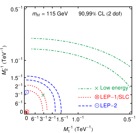
(a)    (b)   

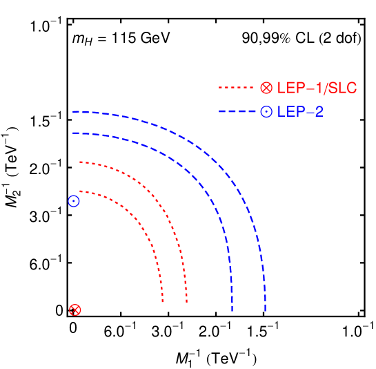
Figure 1: (a) The $1/M_{1}$ vs. $1/M_{2}$ plane showing the results of $2$ parameter $\chi^{2}$ fits to each dataset (low energy, Z-pole and LEP-2). The SM limit is the bottom-left corner. $90$ and $99\%$ C.L. exclusion contours (2 dof) are shown. (b) The $1/M_{1}$ vs. $1/M_{2}$ plane showing only the more constraining Z-pole and LEP-2 fits.

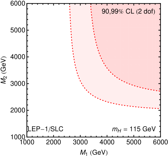
(a)    (b)   

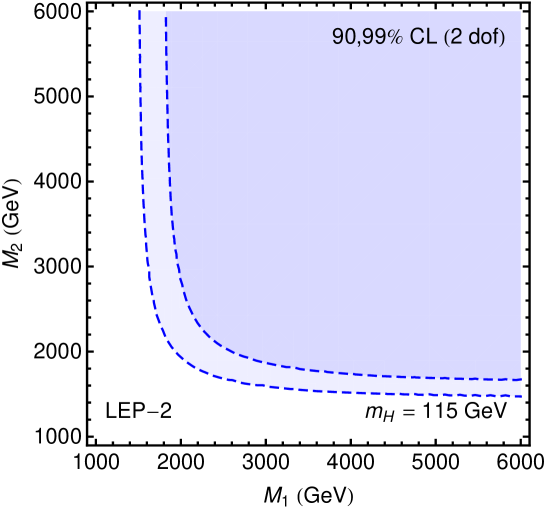
Figure 2: The $M_{1}$ vs. $M_{2}$ plane showing the results of the 2 parameter $\chi^{2}$ fits to the (a) Z-pole and (b) LEP-2 data. $90$ and $99\%$ C.L. exclusion contours (2 dof) are shown in each case.

From Figure 1 we clearly see that the LEP-2 data provide less stringent constraints on the LW masses than the $Z$-pole data. They show a minimum away from the SM corresponding to $M_{1}\to\infty$ and $M_{2}\simeq 2.6$ TeV.

In Figure 2 we invert these plots to show the $90$ and $99\%$ C.L. excluded regions on the $M_{1}$ vs. $M_{2}$ plane. The constraints from the low energy data are not shown as it is clear from Figure 1 that these data only very weakly constrain the model. The tightest constraints come from the $Z$-pole data, however they still potentially allow the LW mass $M_{2}$ to be as low as $M_{1}\simeq 2$ TeV if the other LW mass is $M_{1}\mathrel{\hbox to0.0pt{\raise 2.20013pt\hbox{$>$}\hss}{\lower 2.20013pt\hbox{$\sim$}}}6$ TeV. For the case $M_{1}\simeq M_{2}$ the mass scale $M_{1}\simeq M_{2}\mathrel{\hbox to0.0pt{\raise 2.20013pt\hbox{$<$}\hss}{\lower 2.20013pt\hbox{$\sim$}}}3$ TeV is excluded at 99% C.L. by the $Z$-pole data alone.

As the LW masses are lowered, the observables which are most problematic to the fit are the left-right asymmetry $A^{e}_{LR}$ and the $W$ mass. At $M_{1}=M_{2}=3$ TeV these observables produce pulls of 3.5$\sigma$ and 2.4$\sigma$ respectively. It is interesting to note that these observables also induced sizable pulls in the SM fit. In fact, they are averages of several individual measurements and in the case of the $W$-mass, the measurements from lepton and hadron colliders are only just consistent [31] . It is a curious issue that if only the LEP-2 determination was used then the $W$-mass would fit better in both the SM and the LW extension. There exists a similar situation for the ${\cal A}_{e}(A_{LR}^{f})$ which is an average (assuming lepton universality) of several results obtained at the SLC. The result for ${\cal A}_{e}$ obtained from hadronic final states is quite large when compared to the determinations of ${\cal A}_{\mu,\tau}$ and determination of ${\cal A}_{e}$ from the measurement of $A^{(\tau)}_{\rm pol}$ [30]. It furthermore has quite a small error, the effect of which is to pull the average for ${\cal A}_{e}(A_{LR}^{f})$ away from the SM prediction, and consequently makes the fit to the LWSM worse.

In light of this information, it is tempting to remove the problematic data from the fit. For example, if the $\chi^{2}$ fit is performed without both the TeVatron $W$-mass determination and the${\cal A}_{e}(A_{LR}^{f})$ from SLC then the bounds on the LW masses are weakened. The new fit has a minimum away from the SM, at approximately $M_{1}\simeq 3.3$ TeV and $M_{2}\simeq 8.3$ TeV. The 90 and 99$\%$ C.L. exclusion contours then look rather similar to the LEP-2 constraints and we find that $M_{1}=M_{2}\simeq 2.1$ GeV is not excluded at 99$\%$ C.L.

4 Conclusions

We have analysed the constraints on the LWSM coming from electroweak precision data. We have derived effective electroweak Lagrangians adequate for low energy and the Z-pole (LEP-1/SLC) measurements to all orders in the LW masses at tree level. We have assessed the fit to the LEP-2 data within the oblique approximation. The only non-zero oblique parameters are $Y=-m_{W}^{2}/M_{1}^{2}$ and $W=-m_{W}^{2}/M_{2}^{2}$ [Eq. (69)]. All other oblique parameters, $(\hat{S},X)$ and $(\hat{T},\hat{U},V)$, are found to be zero at the tree level. Our work differs from previous [24] and later work [41] by including effects of contact terms. We find that the latter are of leading order and therefore indispensable as shown in a separate addendum. We have uncovered the negative sign of $W$ and $Y$ as a consequence of the ghost nature of the model, c.f. subsection 2.3.2. In subsection 2.3.1 we have rederived the parameters in the low energy and Z-pole Lagrangians in terms of the oblique parameters in the leading $m_{W}/M_{1,2}^{2}$ approximation.

By performing a $\chi^{2}$ fit we have produced $90\%$ and $99\%$ C.L. exclusion plots for $M_{1}$ and $M_{2}$ which are shown in Fig. 1 (Left). The low energy constraints are considerably weaker than the ones from LEP-1/SLC and LEP-2. Degenerate LW masses $M_{1}=M_{2}\simeq 3\,{\rm TeV}$ are excluded at the $99\%$ confidence level. Somewhat lower values $M_{2}(M_{1})\simeq 2(2.5)\,{\rm TeV}$ are possible when one of the mass scales assumes a very large value.

Studies of $Z^{\prime}$ models [40] would suggest that the resonance like structures of the LW degrees of freedom could be seen at the LHC for masses of up to $\sim 5\,{\rm TeV}$, for an integrated luminosity of $100\,{\rm fb}^{-1}$. On the other hand, the relatively high bounds on the masses point towards the little hierarchy problem, which expresses the dilemma that electroweak data requires typically a light Higgs and sets strong bounds on new degrees of freedom, which were themselves introduced to cure the hierarchy problem. We would like to point out the similarity between the LWSM and models with gauge bosons propagating in a flat extra dimension [33]. Just as in the LWSM, these models do not violate the first two symmetry classes $(+,-)$ and $(-,-)$, described in section 2.3, and therefore the only possible non-vanishing oblique parameters at tree level are $W=Y=(g_{2}v\pi R)^{2}/6=2/3\pi^{2}m_{W}^{2}/M_{KK}^{2}$ (where $R$ is the radius of the extra dimension and $M_{KK}$ is the mass of the first KK mode). The difference between the LWSM and this situation is that $W,Y$ are positive rather than negative and this inverts the role of LEP-2 and LEP-1/SLC data in terms of their constraining role, as can be inferred from the $(W,Y)$ plot in reference [33].

The question of whether quantum field theories of the LW type are consistent or not is interesting independently of their phenomenological aspects. Does the contour deformation [7] lead to a unitary perturbation theory? Is this eventually at the cost of Lorentz invariance [8]? Does microscopic acausality not lead to macroscopic paradoxes? [6]. It is very encouraging that these questions have a positive answers within perturbation theory in the $O(N)$ model in the large $N$ limit [10]. On to other hand, one might also speculate as to whether the LWSM is only an effective description of a theory — potentially with effects which can already be felt by the electroweak precision data investigated in this paper.

Addendum

After this work appeared, a further article, [41] was submitted to arXiv agreeing with the approach of reference [24]. The results of these works differ numerically and conceptually from ours since non-negligible contact terms are omitted.

Before entering into greater detail we would like to emphasize that our results for the oblique parameters, which rely on an expansion in $m_{W,Z}^{2}/M_{\rm LW}^{2}$, are backed-up by an exact treatment of the tree-level low-energy and $Z$-pole effective Lagrangians i.e. our results have also been obtained completely independently of any oblique formalism.

The well-known oblique formalism, as described by Peskin & Takeuchi [36], is suitable for constraining so-called universal models, where all new physics contributions to precision measurements can be described by modifications of the SM gauge boson self energies. The LWSM in the auxiliary field formalism does not belong to this class since there are extra weak gauge bosons of the LW type. In recent years it was realized that theories of this kind can be brought into a universal form if these additional weak gauge bosons couple to the SM fermions in terms of the usual $J_{Y}^{\mu}$ and $J^{\mu}_{a}$ only. This is achieved by integrating out the linear combination of the SM and additional gauge bosons that does not couple to $J_{Y}^{\mu}$ and $J^{\mu}_{a}$, thus avoiding the generation of contact terms (${\cal L}^{\rm eff}\sim J_{Y,a}^{2}$).

In cases like this the new physics can be described by 4 leading parameters, $\hat{S},\hat{T},W,Y$, plus 3 sub-leading parameters, $X,\hat{U},V$. The additional parameters can be seen at the price for taking the contact terms consistently into account. For a concise review on this subject, with many working examples, we refer the reader to Barbieri et al. [33].

The relation between the formalism presented in Barbieri et al [33] and the on-shell formalism used by Peskin & Takeuchi (plus possible contact terms) is worked out in a transparent manner in [42], from where we reproduce the following formulae:

$$\hat{S} = \frac{1}{4s^{2}}\left(\alpha S+4c^{2}\left(\Delta\rho_{*}(0)-\alpha T\right)+\frac{\alpha\delta}{c^{2}}\right)\,,$$ (92)

$$\hat{T} = \Delta\rho_{*}(0)\,,$$ (93)

$$W = \frac{\alpha\delta}{4s^{2}c^{2}}\,,$$ (94)

$$Y = \frac{c^{2}}{s^{2}}\left(\Delta\rho_{*}(0)-\alpha T\right)\,,$$ (95)

or inverted,

$$\alpha S = 4s^{2}\left(\hat{S}-Y-W\right)\,,$$ (96)

$$\alpha T = \hat{T}-\frac{s^{2}}{c^{2}}Y\,,$$ (97)

$$\alpha\delta = 4s^{2}c^{2}W\,,$$ (98)

$$\Delta\rho_{*}(0) = \hat{T}\,,$$ (99)

with $\Delta\rho_{*}(0)\equiv\rho_{*}(0)-1$, c.f. Eq. (3) in our notation. The quantities $\delta\sim W$ and $(\Delta\rho-\alpha T)\sim Y$ parameterize the effects of the charged and neutral current contact terms; c.f formulae (2.9) and (2.10) in reference [42].

In references [24, 41] only the LW gauge bosons were integrated out and it was assumed that the contact terms are negligible. This is explicitly stated in section III of reference [24]. In reference [41] the same effective action is obtained, from where identical results to [24] follow.

Using the results obtained in this paper and Eqs. (94) and (95) it is apparent that the contact terms are of leading order and are therefore not negligible. This can be seen for instance from the rho parameter $\rho_{*}(0)=1+\Delta\rho_{*}(0)$ which is equal to one in our paper with $\hat{T}=0$ (68), but with the un-modified Peskin & Takeuchi formalism $\rho_{*}(0)=1+\alpha T$ [c.f. [36] Eq. (3.13)] it apparently receives a leading order correction since $T\sim m_{W}^{2}/M_{LW}^{2}$ as we shall see below.

Besides low energy physics such as $\rho_{*}(0)$, the contact terms also affect Z-pole physics in an indirect way through a shift in $G_{F}$ which in turn modifies the extraction of the Weinberg angle, e.g. in Eq. (41) or Eq. (3.4) in [36].

In the LWSM, using the formulae (96) and (97), the relations between $S$ and $T$ in the Peskin & Takeuchi formalism and $\hat{S},\hat{T},W,Y$ in the Barbieri et al formalism can be illustrated, allowing a cross-check of the calculations. It is found that

$$S\Big{|}_{\mbox{\small Eq.~{}\eqref{alphaS}}} = \frac{4s^{2}}{\alpha}\left(\frac{m_{W}^{2}}{M_{1}^{2}}+\frac{m_{W}^{2}}{M_{2}^{2}}\right)=4\pi v^{2}\left(\frac{1}{M_{1}^{2}}+\frac{1}{M_{2}^{2}}\right)\,,$$ (100)

$$T\Big{|}_{\mbox{\small Eq.~{}\eqref{alphaT}}} = \frac{s^{2}}{c^{2}\alpha}\frac{m_{W}^{2}}{M_{1}^{2}}=\pi v^{2}\frac{g_{1}^{2}+g_{2}^{2}}{g_{1}^{2}}\frac{1}{M_{1}^{2}}\,,$$ (101)

which does indeed agree with the results of reference [24] Eqs. (7) and (8) and reference [41] in the limit $M_{1}\to\infty$.

The crucial point, and thus the problem with the results of references [24] and [41], is that the constraints on $S$ and $T$ from, for example, the LEP Electroweak Working Group will be produced assuming that the 4-fermion contact terms, parameterized by $W$ (94) and $Y$ (95), are absent or negligible. The important point is that the relations between $S$ and $T$ and the experimental observables will be modified by the non-zero $W$ (94) and $Y$ (95) parameters [or equivalently the non-zero values of $\delta$, Eq. (98), and ($\Delta\rho_{*}(0)-\alpha T$)]. Constraining the LWSM with $S$ and $T$ a la Peskin & Takeuchi is therefore unsuitable, and the cause of our differences with references [24] and [41].

Appendix A $W,Z,A$ propagators in the HD formalism

The LW $W$-propagator in the HD picture can be derived by taking into consideration the additional kinetic term of the gauge field

$$\delta{\cal L}=\frac{1}{M_{2}^{2}}{\rm Tr}[(\hat{D}\hat{W})_{\mu}^{2}]\,,$$ (A.1)

and the Higgs field

$$\delta{\cal L}=-\frac{1}{M_{H}^{2}}\hat{D}^{2}\hat{H}(\hat{D}^{2}\hat{H})^{\dagger}\,.$$ (A.2)

We also introduce a standard $R_{\xi}$ gauge fixing term

$${\cal L}^{gf}=-\frac{1}{2\xi}(\partial\!\cdot\!\hat{A})^{2}\,.$$ (A.3)

The propagator can then be derived in a straightforward way and is eventually given by

$$\hat{D}^{W}_{\mu\nu}=\frac{i}{p^{2}-m_{W}^{2}-p^{4}/M_{2}^{2}}\Big{(}-g_{\mu\nu}+p_{\mu}p_{\nu}f^{W}_{pp}\Big{)}\,,$$ (A.4)

with

$$f^{W}_{pp}=\frac{M_{2}^{2}((1-\xi)M_{H}^{2}+\xi m_{W}^{2})+M_{H}^{2}p^{2}}{M_{2}^{2}M_{H}^{2}p^{2}+m_{W}^{2}M_{2}^{2}(p^{2}-M_{H}^{2})\xi}\,,$$ (A.5)

where $m_{W}$ is defined in Eq. (31). The propagator reduces to the LW gauge field propagator as given in Eq. (24) of reference [3] in the limit,

$$\lim_{m_{W}^{2}\to 0}f^{W}_{pp}=\frac{1-\xi}{p^{2}}+\frac{\xi}{M_{2}^{2}}\,,$$ (A.6)

where the Higgs VEV vanishes. Moreover, in the LW decoupling limit,

$$\lim_{M_{H}^{2},M_{2}^{2}\to\infty}f^{W}_{pp} = \frac{(1-\xi)}{p^{2}-\xi m_{W}^{2}}\,,$$ (A.7)

the propagator reduces to the standard SM $W$-propagator.

For $M_{1}=M_{2}$, the $Z$-propagator is the same as the $W$-propagator with the simple replacement $m_{W}\to m_{Z}\equiv(g_{2}v/2)/c$. If $M_{1}\neq M_{2}$ then the $(\hat{W}_{3},\hat{B})$ system cannot be simultaneously diagonalised. The propagator in the $(\hat{Z},\hat{A})$-basis is given by

$$\hat{D}_{\mu\nu}^{N}(p^{2})=\hat{D}^{N}(p^{2})\left(-g_{\mu\nu}+p_{\mu}p_{\nu}f^{N}_{pp}\right)\,,$$ (A.8)

where

$$\hat{D}^{N}(p^{2})=i(\Gamma^{-1})\,,\qquad f_{pp}^{N}=\mathbb{I}_{2}-(\mathbb{I}_{2}-X)^{-1}\,,$$

$$\Gamma=p^{2}\mathbb{I}_{2}-m_{0}^{2}-p^{4}R_{W}^{T}M^{-2}R_{W}\,,$$

$$X=\left[\mathbb{I}_{2}-\Gamma^{-1}m_{0}^{2}\left(1-\frac{p^{2}}{M_{H}^{2}}\right)\right]-\frac{1}{\xi}\left[\mathbb{I}_{2}-\Gamma^{-1}\left(\Gamma-\mathbb{I}_{2}p^{2}\right)\right]\,,$$ (A.9)

with

$$m_{0}^{2}=\left(\begin{array}[]{cc}m_{Z}^{2}&0\\ 0&0\end{array}\right)\,,\qquad M^{-2}=\left(\begin{array}[]{cc}1/M_{2}^{2}&0\\ 0&1/M_{1}^{2}\end{array}\right)\,,$$ (A.10)

and $R_{W}$ defined as in Eq. (20). We will not give the explicit form of the matrix $\Gamma^{-1}$ but only the relevant low energy limits

$$\lim_{p^{2}\to 0} (-i)\left(\hat{D}^{N}\right)_{ZZ}=-\frac{1}{m_{Z}^{2}}\,,$$ (A.11)

$$\lim_{p^{2}\to 0} (-i)\left(\hat{D}^{N}\right)_{AA}-\frac{1}{p^{2}}=\left(\frac{c^{2}}{M_{1}^{2}}+\frac{s^{2}}{M_{2}^{2}}\right)\,,$$ (A.12)

$$\lim_{p^{2}\to 0} (-i)\left(\hat{D}^{N}\right)_{ZA}=0\,.$$ (A.13)

Note that the photon pole was explicitly subtracted from Eq. (A.12). The $(Z,Z)$ component Eq. (A.11) is the same as in the SM, whereas the $(A,A)$ component has the expected additional massive particle contribution in addition to the photon which contributes to the low energy effective Lagrangian. The non-diagonal contribution Eq. (A.13) vanishes in the low energy limit. All terms in the non-diagonal part are of course proportional to $M_{1}^{2}-M_{2}^{2}$.

We have given the formal expression for the matrix $f_{pp}^{N}$ related to the $p_{\mu}p_{\nu}$ structure only for completeness. The low energy limits are smooth and do not affect the order ${\cal O}(m_{f}m_{f^{\prime}}/{{m}^{2}_{W,\rm ph}})$ supression.

Appendix B The degenerate case $M_{1}=M_{2}$

When the LW masses, $M_{2}$ and $M_{1}$, of the SU(2)_L and U(1) gauge fields are equal matters become analytically tractable.

B.1 Mass matrix diagonalisation

The heavy neutral gauge boson mass matrix, denoted by

$${\cal M_{B}}^{\prime\prime\prime\prime}=\left(\begin{array}[]{cccc}{{m}^{2}_{Z,\rm ph}}&0&0\\ 0&-{{m}^{2}_{\tilde{A},\rm ph}}&0\\ 0&0&-{{m}^{2}_{\tilde{Z},\rm ph}}\\ \end{array}\right)\,,$$ (B.1)

can be diagonalised by the transformation defined in Eq. (46) with

$$\phi=0\quad\Rightarrow\quad x\equiv\frac{M^{2}}{m_{Z}^{2}}=\left(1+\tanh({\theta})\right)\left(1+\frac{1}{\tanh({\theta})}\right)\,,$$ (B.2)

with masses

$$\frac{{{m}^{2}_{Z,\rm ph}}}{m_{Z}^{2}} =1+\tanh({\theta})=\frac{1}{2}\left(x-\sqrt{x(x-4)}\right)\,,$$

$$\frac{{{m}^{2}_{\tilde{A},\rm ph}}}{m_{Z}^{2}} \,=\,\left(1+\tanh({\theta})\right)\left(1+\frac{1}{\tanh({\theta})}\right)=x\,,$$

$$\frac{{{m}^{2}_{\tilde{Z},\rm ph}}}{m_{Z}^{2}} =1+\frac{1}{\tanh({\theta})}=\frac{1}{2}\left(x+\sqrt{x(x-4)}\right)\,.$$ (B.3)

We have denoted $x\equiv x_{1}=x_{2}$ in the degenerate limit. Its analytical expression is the $\phi\to 0$ limit of the expression given in Eq. (2.2.1). The value for $M_{Z}^{2}$ in Eq. (B.1) is of course the limit of the general expression for $M_{Z}^{2}$ given in Eq. (52). The combined transformation $S\cdot Q$ (c.f. Eqs.(20) and (46)) is used to parameterize the diagonalization and $\phi=0$ if and only if $M_{1}=M_{2}$ which is due to the fact that in this case the transformation

$$S^{\prime}=R_{W}\otimes\mathbb{I}_{2}\,,$$

decouples or diagonalizes the photon and the LW photon immediately. This leaves behind a reduced $2\times 2$ matrix which is then diagonalized by the single hyperbolic rotation angle $\theta$. This system is then algebraically identical to the $W$ system discussed in Chapter 2.4.2 in [18] for instance.

B.2 The Z-pole effective Lagrangian in the HD formalism

The purpose of this subsection is to derive the Z-pole effective Lagrangian (the same as in section 2.2.2) in a simpified and therefore more transparent setup. For the case $M_{1}=M_{2}$ the higher deriavtive propagator can be diagonalized in the $(\hat{Z},\hat{A})$ space c.f. appendix A. The couplings of the gauge boson to the currents are left unchanged up to corrections of order ${\cal O}(m_{f}^{2}/M_{f}^{2})$. The Weinberg angle keeps its original meaning and this leads to the prediction

$$s_{*}^{2}({{m}_{Z,\rm ph}})=s^{2}\,,$$

which is indeed verified in the limit $\phi\to 0$ c.f. Eq. (52). We will uncover the parameter $\rho_{f}$ as a multiplicative factor to the standard propagator. The scalar HD propagator [18] reads

$$\hat{D}(p^{2})=\frac{i}{p^{2}-p^{4}/M^{2}-m^{2}}=\frac{-iM^{2}}{(p^{2}-m_{\rm ph}^{2})(p^{2}-M_{\rm ph}^{2})}\,.$$ (B.4)

The analogue of the matching equation (56) for $\rho_{f}$ in the case $M_{1}=M_{2}$ then looks like

$$\lim_{p^{2}\to{{m}^{2}_{Z,\rm ph}}}(-i)\hat{D}(p^{2})\left(p^{2}-{{m}^{2}_{Z,\rm ph}}\right)=\rho_{f}\,\underbrace{\left(4{{m}^{2}_{Z,\rm ph}}\sqrt{2}G_{F}\right)\frac{c^{2}}{g_{2}^{2}}}_{1+\delta_{Z}}\,.$$ (B.5)

This leads to

$$\rho_{f}(1+\delta_{Z}) = \frac{-M^{2}}{{{m}^{2}_{Z,\rm ph}}-{{m}^{2}_{\tilde{Z},\rm ph}}}\ =\ \frac{{{m}^{2}_{\tilde{Z},\rm ph}}+{{m}^{2}_{Z,\rm ph}}}{{{m}^{2}_{\tilde{Z},\rm ph}}-{{m}^{2}_{Z,\rm ph}}}\ =\ \frac{x}{\sqrt{x(x-4)}}$$ (B.6)

$$= \frac{2+\tanh({\theta})+\tanh({\theta})^{-1}}{\tanh({\theta})-\tanh({\theta})^{-1}}\ =\ \cosh^{2}(\theta)(1+\tanh({\theta}))^{2}\,,$$

where we have used used Eq. (B.1) in transforming it to its final form. This leads to

$$\rho_{f}=\cosh^{2}(\theta)(1+\tanh({\theta}))\,,$$ (B.7)

in accordance with Eq.(52) in the limit $\phi\to 0$. The factor $\rho_{f}(1+\delta_{Z})$ is in fact the scaling factor due to hyperbolic rotations. In reference [18] we have denoted it by $s_{(A-\tilde{A})^{2}}$ and indeed

$$s_{(Z-\tilde{Z})^{2}}\equiv\frac{1+r_{Z}^{2}}{1-r_{Z}^{2}}=\rho_{f}(1+\delta_{Z})\,,$$ (B.8)

with the notation $r_{Z}\equiv{{m}_{Z,\rm ph}}/{{m}_{\tilde{Z},\rm ph}}$ and using Eq. (B.6). In the simplified case $M_{1}=M_{2}$ discussed here it is most transparent that $\rho_{f}\geq 1$ in Eq. (B.7) since it is easily deduced from Eq. (B.1) that $1+\tanh({\theta})$ takes values in the range $[2,1[$ when $x$ is constrained to be in its allowed region $[4,\infty[$.

Appendix C Z pole observables

In this appendix we define the Z-pole observables used throughout section 3 to constrain the mass scales of the LW electroweak gauge boson masses. The Z-pole observables are defined from the decay rates of the Z boson and various asymmetries in the cross section for $e^{+}e^{-}\to\bar{f}f$ at a centre of mass energy equal to the mass of the $Z$ boson.

C.1 Ratios of decay rates

The ratios $R_{f}$, which are a direct extension of the famous $R$ function to the Z pole, are defined from the decay rates

$$\Gamma_{Z}^{f}\equiv\Gamma(Z\to\bar{f}f)\quad{\rm and}\quad\Gamma_{Z}^{\rm had}=\sum_{f=u,d,s,c,b}\Gamma(Z\to\bar{f}f)\,,$$ (C.1)

where the tree level expression for the rate has been given in Eq. (85). The leptonic ratios $R_{e,\mu,\tau}$ and the quark ratios $R_{c,b}$ are given by

$$R_{e,\mu,\tau}=\frac{\Gamma_{Z}^{\rm had}}{\Gamma_{Z}^{e,\mu,\tau}}\,,\qquad R_{c,b}=\frac{\Gamma_{Z}^{c,b}}{\Gamma_{Z}^{\rm had}}\,.$$ (C.2)

The total Z decay rate is given as the sum of the leptonic and hadronic rate

$$\Gamma_{Z}=\Gamma_{Z}^{l}+\Gamma_{Z}^{\rm had}+3\Gamma_{Z}^{\bar{\nu}\nu}\,.$$ (C.3)

C.2 Cross-sections & Asymmetries

C.2.1 General defintions

Introducing the following shorthand notation for the cross section for $e^{+}e^{-}\to\bar{f}f$

$$\sigma_{f}\equiv\sigma(e^{+}e^{-}\to\bar{f}f)\,,$$ (C.4)

the peak cross section is simply the cross section at a centre of mass energy equal to the Z boson mass

$$\sigma_{f}^{\rm peak}=\sigma_{f}(s={{m}^{2}_{Z,\rm ph}})\,.$$ (C.5)

It is possible to define five types of asymmetries by combining cross sections for events in the forward and backward hemispheres, and events with differing initial and final state polarizations in all possible ways. The forward backward asymmetry,

$$A_{FB}^{f}\equiv\frac{\sigma_{F}^{f}-\sigma_{B}^{f}}{\sigma_{F}^{f}+\sigma_{B}^{f}}\,,$$ (C.6)

is defined as the normalized difference of the cross-sections for the electron-like fermion going into the forward and backward hemispheres.

The polarization of the initial state electron is used to define the left-right asymmetry,

$$A_{\rm LR}\equiv\frac{\sigma_{L}^{f}-\sigma_{R}^{f}}{\sigma_{L}^{f}+\sigma_{R}^{f}}\,,$$ (C.7)

as the normalized difference of the cross-sections for scattering with left and right handed electrons. These two asymmetries can also be combined into,

$$A_{\rm FBLR}\equiv\frac{(\sigma_{F}-\sigma_{B})_{L}^{f}-(\sigma_{F}-\sigma_{B})_{R}^{f}}{(\sigma_{F}-\sigma_{B})_{L}^{f}+(\sigma_{F}-\sigma_{B})_{R}^{f}}\,,$$ (C.8)

the forward backward left-right asymmetry. We have assumed maximal polarization in Eqs. (C.7) and (C.8) c.f. for example [30] Eqs. (1.58) and (1.59) for more details.

If the polarization of the final state can be measured, as it was possible at the SLAC large detector (SLD) with $\tau$ leptons, then an analoguous asymmetry can be defined for them as well. The final state left right asymmetry is defined

$$A_{rl}^{\tau}\equiv A_{\rm pol}^{(\tau)}\equiv\langle P_{\tau}\rangle\equiv\frac{\sigma_{r}^{\tau}-\sigma_{l}^{\tau}}{\sigma_{r}^{\tau}+\sigma_{r}^{\tau}}\,,$$ (C.9)

and the forward backward asymmetry is defined

$$A_{\rm FB}^{\rm pol}\equiv\frac{(\sigma_{r}-\sigma_{l})_{F}^{\tau}-(\sigma_{r}-\sigma_{l})_{B}^{\tau}}{(\sigma_{r}-\sigma_{l})_{F}^{\tau}+(\sigma_{r}-\sigma_{l})_{B}^{\tau}}\,.$$ (C.10)

C.3 Results at the Z-pole

At the Z-pole the asymmetries and the peak cross sections assume a very simple form, since we can neglect photon-photon and Z-photon exchange terms. The peak cross section is simply given by

$$\sigma_{f}^{\rm peak}=\frac{12\pi}{{{m}^{2}_{Z,\rm ph}}}\frac{\Gamma_{Z}^{e}\Gamma_{Z}^{f}}{\Gamma_{Z}^{2}}\,.$$ (C.11)

Working at tree level and with zero fermion masses the observables are

$$A_{\rm FB}^{f} = \frac{3}{4}{\cal A}_{e}{\cal A}_{f}$$

$$A_{\rm LR}^{f} = {\cal A}_{e}$$

$$A_{\rm FBLR}^{f} = \frac{3}{4}{\cal A}_{f}$$

$$\langle P_{\tau}\rangle = -{\cal A}_{\tau}$$

$$A_{\rm FB}^{\rm pol} = -\frac{3}{4}{\cal A}_{e}\,,$$ (C.12)

with the notation,

$${\cal A}_{f}\equiv\frac{(g^{f}_{L})^{2}-(g^{f}_{R})^{2}}{(g^{f}_{L})^{2}+(g^{f}_{R})^{2}}\,.$$ (C.13)

C.4 Low energy observables

Low energy electroweak processes particularly sensitive to new physics are $\nu$-nucleon and $\nu$-electron scattering and parity violating electron-hadron interactions parameterized by the following effective Lagrangians [25]

$${\cal L}^{\nu N} = -\frac{G_{F}}{\sqrt{2}}(\bar{\nu}\nu)_{V\!-\!A}\sum_{q=u,d}\big{(}\epsilon_{L}(q)(\bar{q}q)_{V\!-\!A}+\epsilon_{R}(q)(\bar{q}q)_{V\!+\!A}\big{)}\,,$$

$${\cal L}^{\nu_{\mu}e} = -\frac{G_{F}}{\sqrt{2}}(\bar{\nu}\nu)_{V\!-\!A}\big{(}g_{V}^{\nu e}(\bar{e}e)_{V}-g_{A}^{\nu e}(\bar{e}e)_{A}\big{)}\,,$$

$${\cal L}^{eq} = \frac{G_{F}}{\sqrt{2}}\sum_{q=u,d}\big{(}C_{1q}(\bar{e}e)_{A}(\bar{q}q)_{V}+C_{2q}(\bar{e}e)_{V}(\bar{q}q)_{A}\big{)}\,.$$ (C.14)

The parameters of the deep inelastic neutrino scattering Lagrangian $\epsilon_{L(R)}(u(d))$ are determined from ratios of cross sections such as the Llewellyn-Smith ratio, $R_{\nu}$ or the Paschos Wolfenstein ratio, $R^{-}$ [25]. However, instead of the $\epsilon_{L(R)}(u(d))$, we will use the following equivalent but less correlated set parameters

$$g_{L}^{2}\equiv\epsilon_{L}^{2}(u)+\epsilon_{L}^{2}(d)\,,\qquad g_{R}^{2}\equiv\epsilon_{R}^{2}(u)+\epsilon_{R}^{2}(d)\,,$$ (C.15)

and the isospin breaking parameters

$$\theta_{L(R)}\equiv\tan^{-1}\Big{(}\frac{\epsilon_{L(R)(u)}}{\epsilon_{L(R)(d)}}\Big{)}\,,$$ (C.16)

obtained from fits to the data. Information on the parameters $\theta_{L(R)}$ can be obtained by varying the isoscalarity of the nucleon target.

The parameters $g_{V(A)}^{e\nu}$ are obtained from $\nu_{\mu}e\to\nu_{\mu}e$ scattering [25] which is transmitted by a t-channel $Z$ boson at leading order.

There are many types of experiment determining the various linear combinations of the coefficients $C_{(1,2)(u,d)}$ such as polarization experiments of $e_{L(R)}N\to eX$, $e_{L(R)}D\to eX$ or measuring the admixture of a P wave contribution to the 6s ground state of Cesium [25].

References

- [1] T. D. Lee and G. C. Wick, Nucl. Phys. B 9 (1969) 209.
- [2] T. D. Lee and G. C. Wick, Phys. Rev. D 2 (1970) 1033.
- [3] B. Grinstein, D. O’Connell and M. B. Wise, Phys. Rev. D 77 (2008) 025012 [arXiv:0704.1845 [hep-ph]].
- [4] J. R. Espinosa, B. Grinstein, D. O’Connell and M. B. Wise, Phys. Rev. D 77 (2008) 085002 [arXiv:0705.1188 [hep-ph]].
- [5] T. D. Lee, in Proceedings of the International School of Physics ”Ettore Majorana,” Erice, Italy, 1970, edited by A. Zichichi, New York, 1971, 63-93
- [6] S. Coleman, in *Erice 1969, Ettore Majorana School On Subnuclear Phenomena*, New York 1970, 282-327
- [7] R. E. Cutkosky, P. V. Landshoff, D. I. Olive and J. C. Polkinghorne, Nucl. Phys. B 12 (1969) 281.
- [8] N. Nakanishi, Phys. Rev. D 3 (1971) 811. N. Nakanishi, Phys. Rev. D 3 (1971) 3235. N. Nakanishi, Phys. Rev. D 5 (1972) 1968. N. Nakanishi, Prog. Theor. Phys. Suppl. 51 (1972) 1.
- [9] T. D. Lee and G. C. Wick, Phys. Rev. D 3 (1971) 1046.
- [10] B. Grinstein, D. O’Connell and M. B. Wise, arXiv:0805.2156 [hep-th].
- [11] D. G. Boulware and D. J. Gross, Nucl. Phys. B 233 (1984) 1.
- [12] K. Jansen, J. Kuti and C. Liu, Phys. Lett. B 309 (1993) 119 [arXiv:hep-lat/9305003].
- [13] K. Jansen, J. Kuti and C. Liu, Phys. Lett. B 309 (1993) 127 [arXiv:hep-lat/9305004].
- [14] A. van Tonder, M. Dorca Int. J. Mod. Phys. A 22 (2007) 2563 [arXiv:hep-th/0610185].
- [15] T. R. Dulaney and M. B. Wise, Phys. Lett. B 658, 230 (2008) [arXiv:0708.0567 [hep-ph]].
- [16] T. G. Rizzo, JHEP 0706 (2007) 070 [arXiv:0704.3458 [hep-ph]].
- [17] T. G. Rizzo, JHEP 0801 (2008) 042 [arXiv:0712.1791 [hep-ph]].
- [18] F. Krauss, T. E. J. Underwood and R. Zwicky, Phys. Rev. D 77 (2008) 015012 [arXiv:0709.4054 [hep-ph]].
- [19] B. Grinstein and D. O’Connell, Phys. Rev. D 78 (2008) 105005 [arXiv:0801.4034 [hep-ph]].
- [20] B. Grinstein, D. O’Connell and M. B. Wise, Phys. Rev. D 77 (2008) 065010 [arXiv:0710.5528 [hep-ph]].
- [21] E. Gabrielli, Phys. Rev. D 77 (2008) 055020 [arXiv:0712.2208 [hep-ph]].
- [22] F. Wu and M. Zhong, Phys. Lett. B 659 (2008) 694 [arXiv:0705.3287 [hep-ph]].
- [23] F. Wu and M. Zhong, Phys. Rev. D 78 (2008) 085010 [arXiv:0807.0132 [hep-ph]].
- [24] E. Alvarez, L. Da Rold, C. Schat and A. Szynkman, JHEP 0804 (2008) 026 [arXiv:0802.1061 [hep-ph]].
- [25] W. M. Yao et al. [Particle Data Group], J. Phys. G 33 (2006) 1.
- [26] J. Erler, arXiv:hep-ph/0005084.
- [27] J. Erler, private communication.
- [28] [LEP Collaboration], arXiv:hep-ex/0312023.
- [29] C. P. Burgess, S. Godfrey, H. Konig, D. London and I. Maksymyk, Phys. Rev. D 49 (1994) 6115 [arXiv:hep-ph/9312291].
- [30] [ALEPH Collaboration], Phys. Rept. 427 (2006) 257 [arXiv:hep-ex/0509008].
- [31] http://lepewwg.web.cern.ch/LEPEWWG/plots/winter2008/
- [32] M. W. Krasny, F. Fayette, W. Placzek and A. Siodmok, Eur. Phys. J. C 51 (2007) 607 [arXiv:hep-ph/0702251].
- [33] R. Barbieri, A. Pomarol, R. Rattazzi and A. Strumia, Nucl. Phys. B 703 (2004) 127 [arXiv:hep-ph/0405040].
- [34] G. Cacciapaglia, C. Csaki, G. Marandella and A. Strumia, Phys. Rev. D 74 (2006) 033011 [arXiv:hep-ph/0604111].
- [35] I. Maksymyk, C. P. Burgess and D. London, Phys. Rev. D 50 (1994) 529 [arXiv:hep-ph/9306267].
- [36] M. E. Peskin and T. Takeuchi, Phys. Rev. D 46 (1992) 381.
- [37] M. J. G. Veltman, Acta Phys. Polon. B 8 (1977) 475.
- [38] P. Sikivie, L. Susskind, M. B. Voloshin and V. I. Zakharov, Nucl. Phys. B 173 (1980) 189.
- [39] [CDF Collaboration], arXiv:0803.1683 [hep-ex].
- [40] M. Dittmar, A. S. Nicollerat and A. Djouadi, Phys. Lett. B 583 (2004) 111 [arXiv:hep-ph/0307020].
- [41] C. D. Carone and R. F. Lebed, Phys. Lett. B 668 (2008) 221 [arXiv:0806.4555 [hep-ph]].
- [42] R. S. Chivukula, E. H. Simmons, H. J. He, M. Kurachi and M. Tanabashi, Phys. Lett. B 603 (2004) 210 [arXiv:hep-ph/0408262].