Spontaneous dissipation of elastic energy by self-localizing thermal runaway

Abstract

Thermal runaway instability induced by material softening due to shear heating represents a potential mechanism for mechanical failure of viscoelastic solids. In this work we present a model based on a continuum formulation of a viscoelastic material with Arrhenius dependence of viscosity on temperature, and investigate the behavior of the thermal runaway phenomenon by analytical and numerical methods. Approximate analytical descriptions of the problem reveal that onset of thermal runaway instability is controlled by only two dimensionless combinations of physical parameters. Numerical simulations of the model independently verify these analytical results and allow a quantitative examination of the complete time evolutions of the shear stress and the spatial distributions of temperature and displacement during runaway instability. Thus we find that thermal runaway processes may well develop under nonadiabatic conditions. Moreover, nonadiabaticity of the unstable runaway mode leads to continuous and extreme localization of the strain and temperature profiles in space, demonstrating that the thermal runaway process can cause shear banding. Examples of time evolutions of the spatial distribution of the shear displacement between the interior of the shear band and the essentially nondeforming material outside are presented. Finally, a simple relation between evolution of shear stress, displacement, shear-band width and temperature rise during runaway instability is given.

I Introduction

Many materials are known to exhibit fracture phenomena that, in apparent contradiction to the expected failure behavior usually associated with plastic yielding or brittle cracking, are characterized by shear deformation localized along a single or a few bands. Ordinarily, one would expect brittle fracture to occur by the opening of microscopic cracks along the fault plane, while conventional plastic yielding associated with deformation of crystals is known to be pervasive and involve work-hardening which seem to be incompatible with the localization of the deformation in shear bands indicating some form of work-softening. This distinct mode of shear failure is observed in a variety of materials, including some amorphous solids such as polymers Lu ; Li ; Cross and bulk metallic glasses Greer ; Wright ; Lewandowski ; Hays , rocks under high confining pressure Obata ; Renshaw ; Wiens and crystalline solids deformed rapidly in impact experiments Miller ; TWWright .

The formation of shear bands in bulk metallic glasses and rocks under high confinement have attracted much attention because, in these materials, the mechanism responsible for the weakening of the material in the bands often initiate instabilities that lead to catastrophic shear failure along one dominant band. Accordingly, shear banding represents the primary mode of failure in many of these material systems. Experimental studies of fracture surfaces of rock samples subjected to high confining pressures demonstrate that the region near the dominant band is essentially devoid of microcracks Renshaw ; Schulson , pointing towards a mechanism leading to viscous sliding without cracking. Similarly, studies of fracture surfaces of metallic glass samples suggest that catastrophic failure is attributable to a large decrease of the viscosity of the material in the catastrophic shear band Wright ; Pampillo . As a consequence, these materials appear to fail in a globally brittle, but locally ductile, manner. The shear bands in metallic glasses, 10–20 nm thick Pekarskaya , seem to be accompanied by significant local increases in temperature. Vein patterns and solidified drops on the fracture surfaces Wright ; Hays ; Bengus indicative of melting of material during catastrophic failure as well as indirect experimental measurements of temperature rises during shear-band operation Lewandowski lend support to this view. Similarly, localized shear failure occurring in the deeper parts of the Earth’s lithosphere, believed to be related to earthquakes located several tens of kilometers below the Earth’s surface, may involve substantial rises in temperature. Geological field observations of melted rock in the form of cm thick pseudotachylyte layers along shear faults provide evidence for considerable heat dissipation during such failure Obata ; Torgeir ; Haakon ; Timm . The catastrophic shear failure process thus seems to be characterized by spontaneous release of a substantial proportion of the stored elastic energy as heat in the region of the rapidly forming shear band.

Apart from the observed differences in the qualitative macroscopic features of localized shear failure as compared to ordinary brittle and plastic failure behaviors, the circumstances under which shear failure seem to occur indicate that this mode of failure may not be ascribed to the conventional mechanisms of opening of microscopic cracks or crystallographic slip by dislocation motion. For instance, the closure of cracks at high confining pressures, non-planar crystal structure of minerals and disorder of mineral grain orientations are all factors that inhibit these mechanisms from operating in rocks in the Earth’s interior. In metallic glasses the high degree of structural disorder cause dislocations to experience a large number of obstacles, reducing their mobility and inhibiting plastic flow. Because of the absence of these basic weakening mechanisms, mantle rocks and bulk metallic glasses can demonstrate exceptionally high strengths. However, although these materials have strengths approaching the theoretical shear strength limit at which atomic bonds break Frenkel , the fact that shear-band thicknesses are usually much larger than interatomic spacing suggests the existence of alternative mechanisms responsible for the catastrophic shear failure. In metallic glasses it has been proposed that granular structure on the microscopic scale may be largely involved in determining the finite width of a shear band Zhang . Discrete element modeling have shown that granular packings subjected to compression may fail by the formation of shear bands or faults due to dilatancy, predicting a shear-band width of about ten grain diameters Astrom ; Francois . However, experimental investigations of deformation in a class of shear yielding polymers Lu show that, despite of the fact that the molecular and microstructural deformation mechanisms are rather different, the phenomenon of shear banding in these materials is strikingly similar to the localization of deformation in metallic materials. This suggests that the general large-scale features of the shear banding phenomenon might be appropriately modeled using a continuum formulation as long as the grain size is small.

Several earlier works have investigated the possibility of shear failure induced by softening mechanisms facilitating ductile or plastic-like deformation. Mainly two explanations have been proposed for the observed localization of shear Pampillo ; Molinari ; Johnson ; Schuh . The first, based on various micromechanical theories developed by Spaepen, Argon, Falk and Langer, and others in order to describe plasticity in amorphous materials Zhang ; Johnson ; Spaepen ; Argon ; ArgonShi ; FalkLanger ; Langer ; Greer09 , suggests that material softening due to structural changes is a mechanism for strain localization. In this case it is usually assumed that the local heat generation during deformation is only a secondary effect and is important to the evolution of the material in the bands only in the later stages of slip. In a recent work, however, Manning, Langer and Carlson Manning proposed that the heat generated by plastic deformation is dissipated in the system’s configurational degrees of freedom and raises an effective temperature rather than the usual kinetic temperature. Thus it was shown that the effective temperature could provide a mechanism for strain localization.

The second explanation, first proposed by Griggs and Baker Griggs and later developed by Ogawa Ogawa in order to explain the occurrence of deep-focus earthquakes, introduces the concept of thermal softening according to which the material is weakened primarily due to the effect of local heating. Local heating increases the temperature which leads to a corresponding decrease in the strongly temperature dependent viscosity. Recent theoretical results BP have demonstrated that, even under nonadiabatic conditions, the thermal softening mechanism may induce a thermal runaway instability exhibiting progressive strain localization, thus leading to shear-band formation and consequent material failure. These results are apparently consistent with experimental results on bulk metallic glasses Lewandowski ; Zhurkin showing that shear-band operation cannot be fully adiabatic.

In the present work we expand on the theoretical investigations of thermal runaway instability in solids, already presented in abbreviated form in Ref. [BP, ]. Our model is based on a simple continuum formulation of a viscoelastic medium, i.e., the rheology contains both viscous and elastic components. The viscous material response is supposed to be induced by thermally activated processes, yielding a strongly temperature dependent viscosity. Thus the model accounts for nonelastic mechanical responses shown by real materials even below the conventional elastic limit, such as the well-known phenomena of creep or relaxation. The temperature in the system is given by the equation for energy conservation. The viscoelastic rheology equation, governing the mechanical behavior of the material, is then coupled to the energy conservation equation through temperature dependent viscosity. We shall make the assumption that initiation of localized deformation is triggered by small (but macroscopic) local heterogeneities or thermal fluctuations in the otherwise large-scale homogeneous and isotropic material. Hence, an increase in strain rate in a weaker zone may cause a local temperature rise due to viscous dissipation, which weakens the zone even further. As a consequence, the local increase in strain rate and temperature may amplify strongly because of the effect of shear heating-induced thermal softening of the material. Accordingly, catastrophic shear failure may occur as a result of thermal runaway instability.

The paper is organized as follows. In Sec. II a simple viscoelastic model is introduced and the basic governing equations are formulated. In Sec. III analytical methods are used to derive the condition for thermal runaway to occur in the adiabatic limit and to estimate the resulting adiabatic temperature rise. Sec. IV presents a linear analysis for the purpose of determining the conditions necessary for thermal runaway to occur for the general case by taking into account the effects of thermal conduction. Numerical solutions to the exact equations are presented in Sec. V, allowing us to quantify the later stages of the thermal runaway process and, in particular, the effects of thermal diffusion will be addressed. We proceed in Sec. VI to derive analytically a relatively simple relation between the evolution of stress, displacement and temperature rise inside the shear band for an adiabatic runaway process. The accuracy of this relation is then evaluated by comparing it to the numerical results for nonadiabatic processes. Finally, we summarize the main conclusions in Sec VII.

II Model

We consider a model consisting of an infinite viscoelastic slab having a finite width $L$ in the $x$-direction; i.e., the geometry is that of a solid bounded by a pair of parallel infinite planes (see Fig. 1). We assume that the slab is in a condition of simple shear such that the only nonzero component of the displacement field is the y-component, which we denote by $u$. Then the shear stress $\sigma_{xy}(=\sigma_{yx})$, hereafter denoted by $\sigma$, is constant throughout the slab and hence only a function of the time $t$ (see Eq. (1) below). Our purpose is to examine spontaneous modes of internal failure in the slab. Therefore, in order to eliminate any additional effects of far-field deformation that could either aid or trigger failure, we impose zero velocity at the slab’s boundaries while we assume that the initial shear stress in the slab is $\sigma_{0}$. It is thus assumed that the shear stress ${\sigma}$ has attained a value $\sigma_{0}$ at $t=0$ regardless of the slab’s loading history which is not considered in the present model. Accordingly, the shear stress in the slab decreases with time from it’s maximum value $\sigma_{0}$ due to relaxation and viscous deformation in the interior. Our particular model setup with zero velocity boundary conditions amounts to searching for the ultimate conditions for which the slab will fail, that is, if it fails at these conditions it is expected to fail earlier at any others. The temperature $T$ in the slab initially equals a background temperature $T_{bg}$ except in the small central region having width $h$ and a slightly elevated temperature $T_{0}$. The small thermal perturbation introduced in the central region ensures that initiation of localized deformation occurs in the neighborhood of the slab’s center. The boundaries ($x=\pm L/2$) are maintained at the temperature $T_{bg}$.

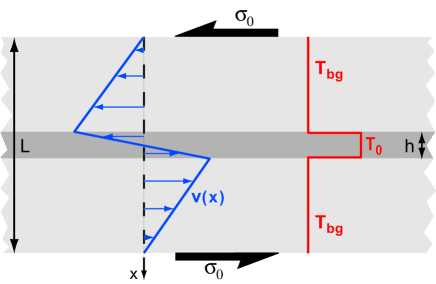
Figure 1: (Color online) Initial setup of the viscoelastic slab model discussed in the text (cross-section in the $xy$-plane). The slab is in a state of stress of simple shear with zero velocity ($v=0$) boundary conditions. The shear stress $\sigma$, constant throughout the slab, initially ($t=0$) equals the value $\sigma_{0}$. The lines show the initial velocity, $v(x)$, and temperature, $T(x)$, profiles. The shaded region illustrates a small perturbation in temperature $T=T_{0}$ of width $h$ at the slab center. Elsewhere, the background temperature is $T=T_{bg}$. The geometry of the strain rate profile concurs with that of the temperature profile.

Assuming inertial effects are negligible, it follows from the translational symmetry in the y- and z-directions of the present model that the shear stress must satisfy the reduced equation for conservation of momentum

$$\frac{\partial\sigma}{\partial x}=0\,,$$ (1)

showing that $\sigma$ is independent of $x$. Without loss of generality the remaining components of the stress tensor are regarded as zero. The viscoelastic rheology is represented by the Maxwell model Malvern for which the strain rate is given by

$$\frac{\partial v}{\partial x}=\frac{1}{\mu(T,\sigma)}\sigma+\frac{1}{G}\frac{\partial\sigma}{\partial t}\,.$$ (2)

Here $v(x,t)$ is the velocity in the y-direction, $G$ is the constant shear modulus and $\mu(T,\sigma)$ is the viscosity. The first and the last term on the r.h.s. of the equation represent the viscous and elastic components of the strain rate, respectively. Assuming that the viscosity of the material is governed by thermally activated processes, the functional dependence of the viscosity on temperature and shear stress may be approximated as

$$\mu(T,\sigma)=A^{-1}e^{E/RT}\sigma^{1-n}\,.$$ (3)

Here $A^{-1}$ is a pre-exponential constant, $n$ is a constant characterizing the dominant creep mechanism, $E$ is the activation energy of creep and $R=8.3$ JK^-1mole^-1 is the universal gas constant. Thus the viscosity has Arrhenius dependence on temperature and it is, in general, a non-linear function of the shear stress.

We simplify the mathematical problem by integration of Eq. (2) to eliminate the velocity from the system of equations. Utilizing the zero velocity boundary conditions, this gives

$$\int_{-\frac{L}{2}}^{\frac{L}{2}}Ae^{-\frac{E}{RT}}\sigma^{n}+\frac{1}{G}\frac{\partial\sigma}{\partial t}dx=\int_{-\frac{L}{2}}^{\frac{L}{2}}\frac{\partial v}{\partial x}dx=0\,,$$ (4)

and we thus obtain the equation which governs the time-dependence of $\sigma$:

$$\frac{\partial\sigma}{\partial t} = -\frac{GA}{L}\sigma^{n}\int_{-\frac{L}{2}}^{\frac{L}{2}}e^{-\frac{E}{RT}}dx\,.$$ (5)

The temperature is determined by the equation for energy conservation

$$\frac{\partial T}{\partial t} = \kappa\frac{\partial^{2}T}{\partial x^{2}}+\frac{1}{C}\sigma\left(\frac{\partial v}{\partial x}-\frac{1}{G}\frac{\partial\sigma}{\partial t}\right)\,,$$ (6)

where $\kappa$ is the thermal diffusivity and $C$ denotes the heat capacity per volume. The last term in Eq. (6) accounts for dissipation in the system and thus includes only the viscous part of the strain rate. Upon substituting for $\partial v/\partial x$ the expression in Eq. (2), the energy equation becomes

$$\frac{\partial T}{\partial t} = \kappa\frac{\partial^{2}T}{\partial x^{2}}+\frac{A}{C}\sigma^{n+1}e^{-\frac{E}{RT}}\,.$$ (7)

Equations (5) and (7) with the specified initial and boundary conditions constitute a closed set of equations for $T(x,t)$ and $\sigma(t)$. These two equations provide the mathematical basis for calculating all the quantities of interest during the deformation process since, from the solutions to these equations for $T$ and $\sigma$, one may calculate the strain rate directly from Eq. (2). We note that, because $\sigma(t)$ is independent of $x$, it follows from Eq. (2) that the geometry of the strain rate profile at any instant concurs with that of the temperature profile $T(x,t)$.

From the considerations above it is clear that we can infer important information about the deformation processes by studying the temperature rises in the system. Useful analytical results can be obtained by invoking approximations appropriate for describing the initial stages of evolutions of $T$ and $\sigma$ for which temperature rises are comparatively small. If instabilities develop, substantial temperature rises are possible, but correspondingly large decreases in shear stress act against unlimited growth. Therefore, to quantify the later stages of the thermal runaway processes, we shall take the maximum temperature rise, defined as

$$\Delta T_{max}=T_{max}-T_{0}\,,$$ (8)

where $T_{max}$ is the maximum temperature with respect to both time and position, as the appropriate physical quantity to study. We solve the system of equations (5) and (7) and estimate $\Delta T_{max}$ using approximate analytical (Sec. III and IV) and numerical (Sec. V) methods.

III Adiabatic case

Important insight into the viscoelastic model is gained by first examining the limiting case of adiabatic heating for which the first term on the r.h.s. of Eq. (7) is neglected. Then the temperature is determined by the reduced equation

$$\frac{\partial T}{\partial t}=\frac{A}{C}\sigma^{n+1}e^{-\frac{E}{RT}}\,.$$ (9)

III.1 Analytical solution

As aid towards understanding the slab’s deformation behavior, we first examine the time evolutions of temperature and shear stress in the initial stages for which temperature changes may be considered comparatively small. In this limit it is possible to obtain approximate analytical solutions to elucidate the deformation problem.

As a first approximation, we insert the initial condition for $T$ in Eq. (5) and perform the integration over space to obtain

$$\frac{\partial\sigma}{\partial t}=-GAe^{-\frac{E}{RT_{0}}}\Delta_{p}\sigma^{n}\,,$$ (10)

where

$$\Delta_{p}=\frac{h}{L}+\left(1-\frac{h}{L}\right)\frac{\mu(T_{0},\sigma_{0})}{\mu(T_{bg},\sigma_{0})}$$ (11)

is a factor which characterizes the initial perturbation. At this point, it is convenient to introduce the quantity $\mu_{0}\equiv\mu(T_{0},\sigma_{0})$ and the dimensionless stress and time

$$\tilde{\sigma}=\frac{\sigma}{\sigma_{0}}\,,\ \ \tilde{t}=\frac{t}{\tau_{r}}\,,$$ (12)

with

$$\tau_{r}=\frac{\mu_{0}}{2G\Delta_{p}}$$ (13)

denoting a characteristic time for stress relaxation in the system. The simplified dimensionless form of the equation is thus

$$\frac{\partial\tilde{\sigma}}{\partial\tilde{t}}=-\frac{1}{2}\tilde{\sigma}^{n}\,.$$ (14)

This equation can be integrated directly by separation of variables and, for the initial condition $\tilde{\sigma}=1$, the corresponding solutions are

$$\tilde{\sigma}=e^{-\frac{1}{2}\tilde{t}}\,,\ \ \ \ n=1\,,$$ (15)

and

$$\tilde{\sigma}=\left[\frac{n-1}{2}\tilde{t}+1\right]^{\frac{1}{1-n}}\,,\ \ \ \ n>1\,.$$ (16)

Another simplification follows from Taylor expanding $1/T$ to first order about the initial temperature $T_{0}$ in the central perturbed zone. Using this approximation, the exponential function in Eq. (9) may be written

$$e^{-\frac{E}{RT}}\approx e^{-\frac{E}{RT_{0}}}e^{\frac{E(T-T_{0})}{RT_{0}^{2}}}\,.$$ (17)

Defining the dimensionless temperature

$$\theta=\frac{E(T-T_{0})}{RT_{0}^{2}}\,$$ (18)

and using Eqs. (12) and (17), we can rewrite Eq. (9) on dimensionless form as

$$\frac{\partial\theta}{\partial\tilde{t}}=\left(\frac{\sigma_{0}}{\sigma_{c}}\right)^{2}\tilde{\sigma}^{n+1}e^{\theta}\,,$$ (19)

which must satisfy the initial condition $\theta=0$ in the perturbed zone. Here we have introduced the new quantity

$$\sigma_{c}=\sqrt{2\Delta_{p}\frac{GCR}{E}}T_{0}\,,$$ (20)

having the same dimension as stress. Now, by substituting the solutions (15) and (16) for $\tilde{\sigma}$ in Eq. (19), and once again integrating by separation of variables, we find the solutions

$$\theta=-\ln\left[\left(\frac{\sigma_{0}}{\sigma_{c}}\right)^{2}\left(e^{-\tilde{t}}-1\right)+1\right]\,,\ \ \ \ n=1\,,$$ (21)

and

$$\theta=\mbox{}-\ln\left\{\left(\frac{\sigma_{0}}{\sigma_{c}}\right)^{2}\left[\left(\frac{n-1}{2}\tilde{t}+1\right)^{\frac{2}{1-n}}-1\right]+1\right\}\,,$$

$$n>1\,.$$

(22)

Both solutions (21) and (22) are seen to exhibit two distinct modes of evolution, depending on the value of $\sigma_{0}$. Indeed, the solutions are bounded only if $\sigma_{0}<\sigma_{c}$. If this condition is violated, the temperature grows unlimited at the critical times

$$\tilde{t}_{cr}=-\ln\left[1-\left(\frac{\sigma_{c}}{\sigma_{0}}\right)^{2}\right]\,,\ \ \ \ n=1\,,$$ (23)

and

$$\tilde{t}_{cr}=\frac{2}{n-1}\left\{\left[1-\left(\frac{\sigma_{c}}{\sigma_{0}}\right)^{2}\right]^{\frac{1-n}{2}}-1\right\}\,,\ \ \ \ n>1\,.$$ (24)

The dramatic change in growth of temperature as $\sigma_{0}$ exceeds $\sigma_{c}$ indicates that, under adiabatic conditions, $\sigma_{c}$ plays the role of a critical stress above which thermal runaway occurs.

A few remarks concerning the validity of Eqs. (21)–(24) are appropriate here. The main effects of the approximations adopted in deriving these equations is that the heat production rate becomes too large for large temperature rises and that temperatures may increase without limit. In contrast, the exact equations always give finite values for temperature rises. Nevertheless, solutions (21) and (22) are expected to yield reasonable approximations at least into the very early stages of development of adiabatic thermal runaway. Hence, we also expect that these simplified estimates correctly predict the condition for adiabatic thermal runaway to occur. That this indeed is the case, will be independently verified by numerical methods in section V.

III.2 Maximum temperature rise during adiabatic thermal runaway

We now discuss the later stages of adiabatic thermal runaway, for which the analytical solutions obtained in the previous section are inapplicable. Then, a simple analytical estimate of the maximum temperature rise (Eq. (8)) can be made by considering overall energy balance as follows.

Integration of Eq. (9) over space gives

$$\int_{-\frac{L}{2}}^{\frac{L}{2}}\frac{\partial T}{\partial t}dx=\frac{A}{C}\sigma^{n+1}\int_{-\frac{L}{2}}^{\frac{L}{2}}e^{-\frac{E}{RT}}dx\,.$$ (25)

The expression on the r.h.s. can be obtained from Eq. (5), giving

$$\frac{A}{C}\sigma^{n+1}\int_{-\frac{L}{2}}^{\frac{L}{2}}e^{-\frac{E}{RT}}dx=-\frac{L}{GC}\sigma\frac{\partial\sigma}{\partial t}\,.$$ (26)

Combining Eqs.  (25) and (26) we obtain

$$\frac{\partial}{\partial t}\left[\int_{-\frac{L}{2}}^{\frac{L}{2}}Tdx+\frac{L}{2GC}\sigma^{2}\right]=0\,,$$ (27)

which may be integrated over time to give

$$\int_{-\frac{L}{2}}^{\frac{L}{2}}\Delta T(x,t)dx=\frac{L}{C}\frac{\sigma_{0}^{2}-\sigma(t)^{2}}{2G}\,,$$ (28)

where $\Delta T(x,t)=T(x,t)-T(x,0)$. Now, it is reasonable to assume that the viscous part of the deformation mainly occurs within the initially perturbed zone $|x|\leq h/2$. Then, essentially no heat will be dissipated outside this zone, and because diffusion of heat is assumed negligible for the present case, the temperature rises in these outer regions become vanishingly small. Inside the perturbed region, dissipation of heat is expected to be distributed monotonously. To understand the reason, recall that in this region the initial temperature, and therefore the initial viscosity, are uniformly distributed. Accordingly, as long as the process is adiabatic, the temperature rise in the same region will be approximately uniform, i.e., independent of $x$. As a result, the integral in Eq. (28) may be replaced by a simple integration of uniform temperature rise over the region $|x|\leq h/2$. Performing the integration, we find that the adiabatic maximum temperature rise inside the perturbed region is given by

$$\Delta T_{max}^{a}=\frac{\sigma_{0}^{2}L}{2GCh}.$$ (29)

In writing Eq. (29) we have made the assumption that the runaway process continues until the stress $\sigma(t)$ in the slab is much smaller than $\sigma_{0}$. We recognize the quantity $\sigma_{0}^{2}/2G$ as the elastic energy per unit volume stored in the slab in its initial state. Eq. (29) reflects the fact that during thermal runaway, and under the assumptions made, all the elastic energy in the system spontaneously dissipates uniformly as heat in the initially perturbed zone. As was mentioned earlier, the geometry of the strain rate profile concurs at any instant with that of the temperature profile. An immediate consequence of the adiabatic assumption is therefore that the width of the shear band formed during runaway equals the width of the initially perturbed zone in which the uniform temperature rise occurs. Although the adiabatic approximation provides a simple means to obtain important insight into the process, neglect of thermal diffusion may give misleading results. The extent to which the adiabatic assumption is valid will be investigated by numerical methods in Sec. V.

IV Conditions for thermal runaway. The general case

In this section we attempt to determine the conditions necessary for thermal runaway to occur for the general case by taking into account the effects of thermal conduction. For that purpose, we investigate the stability of the coupled equations (5) and (7) by a linear analysis. Then, as an approximation for the initial stages, we insert the initial conditions for $\sigma$ and $T$ in Eq. (5) and carry out the integration over space to obtain the simplified equation

$$\frac{\partial\sigma}{\partial t}=-\frac{\sigma_{0}}{2\tau_{r}}\,,$$ (30)

which has the solution

$$\sigma(t)=\sigma_{0}\left[1-\frac{t}{2\tau_{r}}\right]\,.$$ (31)

Here $\tau_{r}$ is the relaxation time given by eq. (13). Using this expression, we expand $\sigma^{n+1}$ to first order in time, yielding

$$\sigma(t)^{n+1}\approx\sigma_{0}^{n+1}\left[1-(n+1)\frac{t}{2\tau_{r}}\right]\,.$$ (32)

The expansion is valid for small times $t\ll\tau_{r}$. Equation (7), determining the temperature rise in the system, may now be approximated by substituting for $\sigma^{n+1}$ the result obtained in Eq. (32):

$$\frac{\partial T}{\partial t}=\kappa\frac{\partial^{2}T}{\partial x^{2}}+\frac{\sigma_{0}^{2}}{C\mu_{0}}\left[1-(n+1)\frac{t}{2\tau_{r}}\right]e^{\frac{E}{R}\left(\frac{1}{T_{0}}-\frac{1}{T}\right)}\,.$$ (33)

Our aim is to obtain the conditions for which the perturbation in the central region becomes unstable. Hence, in the following discussion we consider only the temperature inside the central region $|x|\leq h/2$. Assume that the temperature evolution is continuous and smooth and that there exists a steady temperature $T_{ss}$ for which $\partial T_{ss}/\partial t=0$. Then $T_{ss}$ satisfies the reduced equation for steady flow

$$\kappa\frac{\partial^{2}T_{ss}}{\partial x^{2}}=-\frac{\sigma_{0}^{2}}{C\mu_{0}}\left[1-(n+1)\frac{t}{2\tau_{r}}\right]e^{\frac{E}{R}\left(\frac{1}{T_{0}}-\frac{1}{T_{ss}}\right)}\,.$$ (34)

The stability of the steady state solution may be investigated by superposing a perturbation $\delta$ on $T_{ss}$. The resulting non-steady temperature $T=T_{ss}+\delta$ must satisfy Eq. (33), describing time-dependent flow. For simplicity, we restrict the analysis to arbitrarily small $\delta$. In this case, since $\delta/T_{ss}\ll 1$, we have $1/T\approx 1/T_{ss}-\delta/T_{ss}^{2}$, and we obtain for the exponential term in Eq. (33)

$$e^{\frac{E}{R}\left(\frac{1}{T_{0}}-\frac{1}{T}\right)} \approx e^{\frac{E}{R}\left(\frac{1}{T_{0}}-\frac{1}{T_{ss}}\right)}e^{\frac{E\delta}{RT_{ss}^{2}}}$$ (35)

$$\approx e^{\frac{E}{R}\left(\frac{1}{T_{0}}-\frac{1}{T_{ss}}\right)}\left(1-\frac{E\delta}{RT_{ss}^{2}}\right)\,,$$

where we keep only the leading term in the last expansion because $E\delta/RT_{ss}^{2}\ll 1$ for arbitrarily small $\delta$. Using this expansion and utilizing Eq. (34), Eq. (33) reduces to a linearized equation for $\delta$:

$$\frac{\partial\delta}{\partial t} = \kappa\frac{\partial^{2}\delta}{\partial x^{2}}$$

$$+\frac{\sigma_{0}^{2}E}{C\mu_{0}RT_{ss}^{2}}e^{\frac{E}{R}\left(\frac{1}{T_{0}}-\frac{1}{T_{ss}}\right)}\left(1-(n+1)\frac{t}{2\tau_{r}}\right)\delta\,.$$

In our search for spontaneous thermal runaway modes we are interested in finding the conditions for which the initial perturbation $T_{0}$ instantly starts to increase. If we now anticipate that there is a sharp transition boundary between the stable modes, where $T_{0}$ instantly drops, and the unstable modes, where $T_{0}$ instantly grows, one may expect that $T_{0}$ plays the role of a steady state right at the transition boundary. Accordingly, to obtain the conditions for spontaneous runaway modes, one should analyze the case in which the initial perturbation $T_{0}$ itself becomes a steady state and therefore choose $T_{ss}\approx T_{0}$ in Eq. (LABEL:eq:lindeltaone). This yields the equation

$$\frac{\partial\delta}{\partial t}=\kappa\frac{\partial^{2}\delta}{\partial x^{2}}+\frac{\sigma_{0}^{2}E}{C\mu_{0}RT_{0}^{2}}\left(1-(n+1)\frac{t}{2\tau_{r}}\right)\delta\,.$$ (37)

Then, normalizing time by the relaxation time given by Eq. (13), and introducing new dimensionless variables

$$\tilde{\delta}=\frac{\delta}{E/R}\,,\ \ \tilde{x}=\frac{x}{h}\,,$$ (38)

we recast Eq. (37) into dimensionless form as

$$\frac{\partial\tilde{\delta}}{\partial\tilde{t}}=\frac{\tau_{r}}{\tau_{d}}\frac{\partial^{2}\tilde{\delta}}{\partial\tilde{x}^{2}}+\left(\frac{\sigma_{0}}{\sigma_{c}}\right)^{2}\left(1-(n+1)\frac{\tilde{t}}{2}\right)\tilde{\delta}\,.$$ (39)

Here $\tau_{d}=h^{2}/\kappa$ is the characteristic thermal diffusion time for diffusion of heat away from the central region, and $\sigma_{c}$ is the characteristic stress introduced earlier in (20). Note that two combinations of physical parameters appear in this simplified equation, namely $\sigma_{0}/\sigma_{c}$ and $\tau_{r}/\tau_{d}$. The first combination entered the analysis in Sec. III.1, in which it was interpreted as the factor controlling the stability of the system in the adiabatic limit. The second combination, which is the ratio of the relaxation time to the thermal diffusion time, will modify the stability criterion for processes which are not adiabatic. The effect of this dimensionless variable on the conditions for thermal runaway will be addressed in the analysis below.

Assuming, for simplicity, that $\tilde{\delta}$ vanish at the “boundaries” $\tilde{x}=\pm 1/2$ and that $\tilde{\delta}$ is a positive, even function, the general solution to Eq. (39) can be represented as a sum of particular solutions as

$$\tilde{\delta}=\sum_{m=0}^{\infty}f_{m}\left(\tilde{x},\tilde{t}\right)\,,$$ (40)

with

$$f_{m}\left(\tilde{x},\tilde{t}\right) = B_{m}e^{\left[-\frac{\tau_{r}}{\tau_{d}}k_{m}^{2}+\left(\frac{\sigma_{0}}{\sigma_{c}}\right)^{2}\right]\tilde{t}-\left(\frac{\sigma_{0}}{\sigma_{c}}\right)^{2}\frac{(n+1)\tilde{t}^{2}}{4}}$$

$$\times\cos\left(k_{m}\tilde{x}\right)\,.$$

Here $k_{m}=(2m+1)\pi$ denote the frequencies of the perturbation satisfying the required boundary conditions, and $B_{m}$ denote the amplitudes. It follows from the general formula for Fourier cosine coefficients that $B_{m}$ must decrease with increasing $m$. Furthermore, we note that $k_{m}$ increases with increasing $m$. Accordingly, $f_{0}$ is the largest term in the series expansion, and it dominates the stability of the perturbation in (40). To proceed, we must analyze the time evolution of the perturbation, which is controlled by the argument of the exponential in $f_{0}$. For the case when the coefficient in the leading term in the argument is negative or zero, $f_{0}$ becomes a monotonically decreasing function of $\tilde{t}$. As a result, $\tilde{\delta}$ decreases with time, implying a stable situation. In the opposite case, when the coefficient in the leading term of the argument is positive, $f_{0}$ increases with time until it reaches a maximum for which $\partial f_{0}/\partial\tilde{t}=0$. Solving this equation, we obtain the characteristic time

$$\tilde{t}_{max}=\frac{2}{n+1}\left[1-\left(\frac{\sigma_{0}}{\sigma_{c}}\right)^{-2}\frac{\tau_{r}}{\tau_{d}}\pi^{2}\right]$$ (42)

above which the perturbation begins to decrease, and the corresponding maximum of $f_{0}$:

$$f_{0}\left(\tilde{x},\tilde{t}_{max}\right)=B_{0}e^{\frac{1}{n+1}\left(\frac{\sigma_{0}}{\sigma_{c}}\right)^{-2}\left[\left(\frac{\sigma_{0}}{\sigma_{c}}\right)^{2}-\frac{\tau_{r}}{\tau_{d}}\pi^{2}\right]^{2}}\cos\left(\pi\tilde{x}\right)\,.$$

(43)

In Eqs. (42) and (43) we used that $k_{0}=\pi$. Thus, for certain conditions, the solution to this linearized perturbed problem predicts only a limited increase in temperature. Due to the linear approximation of the exponential functions in the linear analysis, however, heat is produced at a rate which is only a linear function of $\tilde{\delta}$. This approximation is only valid for infinitesimal perturbations and severely underestimates the heat production rate as the perturbation grows towards finite amplitudes. Nevertheless, we may assume that if the magnitude of $\tilde{\delta}$ becomes substantial before $\tilde{t}$ approaches the characteristic time $\tilde{t}_{max}$, the perturbation will develop into thermal runaway. To proceed, we therefore investigate the growth of the quantity

$$\left(\frac{f_{0}\left(\tilde{x},\tilde{t}_{max}\right)}{f_{0}\left(\tilde{x},0\right)}\right)^{n+1}=e^{\left(\frac{\sigma_{0}}{\sigma_{c}}\right)^{-2}\left[\left(\frac{\sigma_{0}}{\sigma_{c}}\right)^{2}-\frac{\tau_{r}}{\tau_{d}}\pi^{2}\right]^{2}}\,.$$ (44)

We now anticipate that a thermal runaway will develop if the quantity above amplifies beyond the characteristic factor $e$, leading to the equation

$$\left(\frac{\sigma_{0}}{\sigma_{c}}\right)^{-2}\left[\left(\frac{\sigma_{0}}{\sigma_{c}}\right)^{2}-\frac{\tau_{r}}{\tau_{d}}\pi^{2}\right]^{2}=1\,,$$ (45)

for which the solution is

$$\frac{\sigma_{0}}{\sigma_{c}}=\sqrt{\pi^{2}\frac{\tau_{r}}{\tau_{d}}+\frac{1}{2}\left[1+\sqrt{1+4\pi^{2}\frac{\tau_{r}}{\tau_{d}}}\right]}\,.$$ (46)

The expression in (46) determines the critical values of the dimensionless variables $\sigma_{0}/\sigma_{c}$ and $\tau_{r}/\tau_{d}$ at which the transition between stable modes and unstable thermal runaway modes occurs. Thus, at the transition between the two modes, $\sigma_{0}/\sigma_{c}$ becomes a function of $\tau_{r}/\tau_{d}$. The curve along which the transition occurs divides the $\sigma_{0}/\sigma_{c}$, $\tau_{r}/\tau_{d}$ plane into a “phase diagram”, as illustrated in Fig. 2.

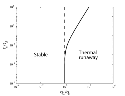
Figure 2: Plots of the critical values of $\sigma_{0}/\sigma_{c}$ defining the transition boundaries between stable deformation modes and unstable thermal runaway modes according to approximate theoretical predictions. The solid curve shows the results of the linear stability analysis taking thermal conduction into account, as given by the expression in Eq. (46). The critical values of $\sigma_{0}/\sigma_{c}$ are seen to increase with increasing $\tau_{r}/\tau_{d}$. The dashed line shows the results of the adiabatic analysis made in Sec. III which completely neglects the effects of thermal conduction and thus predicts a threshold stress which is independent of $\tau_{r}/\tau_{d}$.

As the solid curve in Fig. 2 shows, the critical values of $\sigma_{0}/\sigma_{c}$ increase with increasing $\tau_{r}/\tau_{d}$. However, for $\tau_{r}/\tau_{d}<10^{-2}$ the transition curve stays almost vertical, and the critical $\sigma_{0}/\sigma_{c}$ approximately equals its lower bound. The lower bound is obtained in the limit $\tau_{r}/\tau_{d}\rightarrow 0$ and corresponds to adiabatic processes. In this case Eq. (46) reduces to

$$\sigma_{0}=\sigma_{c}\,,$$ (47)

and we thereby recover the result obtained earlier in Sec. III.1.

Hence, $\sigma_{c}$ is the smallest stress required for spontaneous thermal runaway to occur. We note, however, that the required stress for onset of thermal runaway begins to deviate significantly from $\sigma_{c}$ only when $\tau_{r}/\tau_{d}>1$. Therefore $\sigma_{c}$ provides a good estimate for the critical stress above which thermal runaway occurs as long as $\tau_{r}/\tau_{d}<1$. In this regime, then, onset of thermal runaway is to a good approximation independent of the quantities which control kinetic processes since these quantities do not appear in the expression for $\sigma_{c}$ (see Eq. (20)). The results of this linear stability analysis are consistent with earlier numerical estimates of initial stages of runaway instability in a two-dimensional setup Boris . Explicit estimates of $\sigma_{c}$ were made in Ref. [BP, ] and compared to typical failure stresses in metallic glasses and rocks under high confining pressure, showing that the predicted values of $\sigma_{c}$ are within the correct order of magnitude for such systems.

For the situation when $\tau_{r}/\tau_{d}\gg 1$ the rate of relaxation or creep in the material is very slow compared to the process of thermal diffusion, which means that the heat produced rapidly flows away from the initially perturbed zone. The stress required for thermal runaway to occur in this case is therefore much larger than $\sigma_{c}$.

Finally, it should be mentioned that the linear analysis presented in this section, and leading to Eq. (46), was based on the greatly simplified equations (32) and (37). The correctness of the obtained results must thus be investigated by a proper analysis of the set of the fully coupled equations (5) and (7). Fortunately, as will be demonstrated in Sec. V, the results of the linear analysis are found to agree extremely well with the results obtained from numerical solutions to the complete equations.

V Numerical approach

In order to obtain solutions to the complete equations (5) and (7) without simplifying assumptions we perform numerical simulations. This enables us to capture any nonlinear effects in our thermo-mechanical system and to study the complete time evolution of $T(x,t)$, $\sigma(t)$ and the displacement $u(x,t)$.

V.1 Dimensionless equations

The complexity of the problem can be significantly reduced by introducing dimensionless variables. Inspired by the analysis in sections III and IV, we choose the particular normalization

$$\tilde{\sigma}=\frac{\sigma}{\sigma_{0}}\,,\ \ \tilde{T}=\frac{T}{E/R}\,,\ \ \tilde{t}=\frac{t}{\tau_{r}}\,,\ \ \tilde{x}=\frac{x}{h}\,.$$ (48)

In most situations of interest $T_{bg}\ll E/R$ ($E/R$ is typically of the order of 10000 K), and for simplicity we therefore restrict our numerical analysis to the case $\tilde{T}_{bg}\ll 1$.

The closed set of equations for $T$ and $\sigma$ can then be written on dimensionless form as

$$\frac{\partial\tilde{T}}{\partial\tilde{t}}=\frac{\tau_{r}}{\tau_{d}}\frac{\partial^{2}\tilde{T}}{\partial\tilde{x}^{2}}+\tilde{T}_{0}^{2}\left(\frac{\sigma_{0}}{\sigma_{c}}\right)^{2}\tilde{\sigma}^{n+1}e^{\frac{1}{\tilde{T}_{0}}-\frac{1}{\tilde{T}}}\,,$$ (49)

and

$$\frac{\partial\tilde{\sigma}}{\partial\tilde{t}}=-\frac{1}{2}\frac{h/L}{h/L+\left(1-\frac{h}{L}\right)e^{\frac{1}{\tilde{T}_{0}}-\frac{1}{\tilde{T}_{bg}}}}\int_{-\frac{L}{2h}}^{\frac{L}{2h}}e^{\frac{1}{\tilde{T}_{0}}-\frac{1}{\tilde{T}}}d\tilde{x}\,.$$ (50)

Similarly, the dimensionless form of the rheology equation becomes

$$\frac{\partial\tilde{v}}{\partial\tilde{x}}=e^{\frac{1}{\tilde{T_{0}}}-\frac{1}{\tilde{T}}}\tilde{\sigma}^{n}+2\Delta_{p}\frac{\partial\tilde{\sigma}}{\partial\tilde{t}}\,,$$ (51)

where $\tilde{v}=v/(\sigma_{0}h/\mu_{0})$. Displacements are correspondingly calculated in units of $(\sigma_{0}h/\mu_{0})\tau_{r}=\sigma_{0}h/(2\Delta_{p}G)$.

The utility of this non-dimensionalization procedure lies in that the original problem containing thirteen dimensional parameters now has been reduced to one containing only eight dimensionless parameters (as can be verified upon inspection of the above equations), substantially reducing the number of necessary numerical runs. Moreover, the dimensionless temperature $\tilde{T}$ may now be explicitly expressed as a function of the two combinations of parameters $\tau_{r}/\tau_{d}$ and $\sigma_{0}/\sigma_{c}$ that were suggested by the linear analysis in Sec. IV as controlling parameters for onset of thermal runaway:

$$\tilde{T}=f_{1}\left(\tilde{x},\tilde{t},\tilde{T}_{0},\tilde{T}_{bg},\frac{h}{L},n,\frac{\tau_{r}}{\tau_{d}},\frac{\sigma_{0}}{\sigma_{c}}\right)\,.$$ (52)

To ensure correct numerical results the coupled equations (49) and (50) are solved using a finite-difference method with non-uniform mesh and a tailored variable time-step.

V.2 Temperature rise

Based on the analysis conducted in Sec. V.1, we are now in a position to investigate the thermal runaway phenomenon in a self-consistent manner by numerical calculations of the complete time evolution of $T$ and $\sigma$ with account of heat conduction. Guided by the results obtained in Sec. III, we shall begin by studying the maximum temperature rise $\Delta T_{max}$ (Eq. (8)), normalized by the adiabatic temperature rise $\Delta T_{max}^{a}$ (Eq. (29)), as a function of the governing variables.

The temperature always attains the maximum value at the centre of the slab. Hence, the maximum temperature $T_{max}$ with respect to both time and position must satisfy the equation

$$\left.\frac{\partial T}{\partial t}\right|_{x=0}=0\,,$$ (53)

from which, by use of Eq. (52), it is easy to show that $\Delta\tilde{T}_{max}=\tilde{T}_{max}-\tilde{T}_{0}$ is independent of $\tilde{x}$ and $\tilde{t}$. Then, by rewriting $\Delta T_{max}^{a}$ in terms of dimensionless variables, it is immediately clear that the maximum temperature rise scaled by the adiabatic temperature rise is a function of the remaining six dimensionless variables only, i.e.,

$$\frac{\Delta T_{max}}{\Delta T_{max}^{a}}=f_{2}\left(\tilde{T}_{0},\tilde{T}_{bg},\frac{h}{L},n,\frac{\tau_{r}}{\tau_{d}},\frac{\sigma_{0}}{\sigma_{c}}\right)\,,$$ (54)

simplifying the problem even further.

To examine the behavior of $\Delta T_{max}/\Delta T_{max}^{a}$, we systematically varied all six dimensionless parameters and computed $\Delta T_{max}$ from Eqs. (49) and (50) for each selection of fixed parameter values. We present several sets of numerical runs in Fig. 3 in terms of contour plots of $\Delta T_{max}/\Delta T_{max}^{a}$ versus $\sigma_{0}/\sigma_{c}$ and $\tau_{r}/\tau_{d}$ for different values of the remaining parameters $n$, $L/h$, $\tilde{T}_{bg}$ and $\tilde{T}_{0}$.

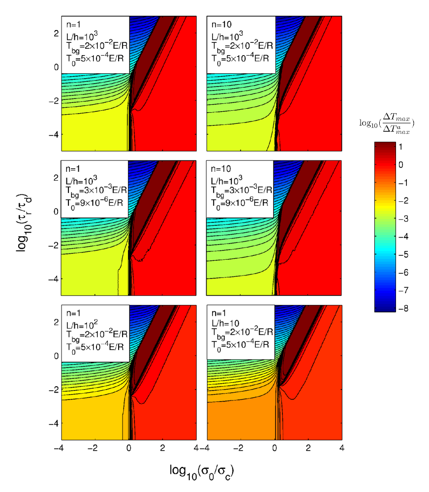
Figure 3: (Color) Contour plots of $\Delta T_{max}/\Delta T_{max}^{a}$ versus $\sigma_{0}/\sigma_{c}$ and $\tau_{r}/\tau_{d}$. Each contour plot represents a set of numerical runs for a certain choice of fixed values for the parameters $n$, $L/h$, $\tilde{T}_{bg}$ and $\tilde{T}_{0}$ (values are specified in white boxes). The collection of the six contour plots thus constitutes a numerical example of independent variations of all the six dimensionless parameters entering Eq. (54). A detailed explanation of a contour plot is given in the caption of Fig. 4.

As the series of contour plots show, $\Delta T_{max}/\Delta T_{max}^{a}$ depends strongly on the two variables $\sigma_{0}/\sigma_{c}$ and $\tau_{r}/\tau_{d}$, but is rather insensitive to variations in the four remaining parameters. In this sense, $\Delta T_{max}/\Delta T_{max}^{a}$, when plotted against the two combinations of parameters $\sigma_{0}/\sigma_{c}$ and $\tau_{r}/\tau_{d}$, closely resembles a data collapse. It has thus been demonstrated that the maximum temperature rise normalized by the adiabatic temperature rise is, to a quite good approximation, a function of the two dimensionless variables $\sigma_{0}/\sigma_{c}$ and $\tau_{r}/\tau_{d}$ alone, as previously suggested by the linear analysis (see Sec. IV).

Having identified the controlling variables for the maximum temperature rise in our system, we can now proceed to study a representative contour plot, shown in Fig. 4, in more detail. As can be seen, the plot exhibits a low-temperature region, corresponding to stable deformation processes, and a high-temperature region, corresponding to thermal runaway processes. As was predicted by the linear analysis in Sec. IV, these two regions are sharply distinguished by a critical boundary (or “transition curve”) dividing the $\sigma_{0}/\sigma_{c}$, $\tau_{r}/\tau_{d}$ plane into a “phase diagram”. The location of the critical boundary correlates well with the analytical predictions, see Fig. 2 for comparison. This verifies that the conditions for spontaneous thermal runaway to occur have been accurately determined. A physical explanation of the stability of the deformation processes in the low-temperature region is that, there, the effects of thermal diffusion and stress relaxation dominate over the positive feedback mechanism. In the high-temperature region the situation is exactly the opposite, leading to instability and consequently thermal runaway. In the following section we turn our attention to the high-temperature region, and we shall in particular discuss the effects of thermal diffusion on thermal runaway processes.

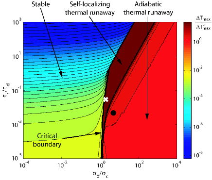
Figure 4: (Color) A representative contour plot of $\Delta T_{max}$ scaled by the adiabatic temperature rise $\Delta T_{max}^{a}$ as a function of the dimensionless variables $\sigma_{0}/\sigma_{c}$ and $\tau_{r}/\tau_{d}$. The dark lines represent contour lines. The plot exhibits mainly two sharply distinguished regions according to small and large temperature rises, thus defining a critical boundary dividing the $\sigma_{0}/\sigma_{c}$, $\tau_{r}/\tau_{d}$ plane into a “phase diagram”. The low-temperature region, denoted “stable” (blue and green colors), represents stable deformation processes. The high-temperature region represents unstable thermal runaway processes and is further subdivided into two domains, denoted by “self-localizing thermal runaway”and “adiabatic thermal runaway” (brown and red color, respectively), which represents runaway processes of different characters (see text). For computational efficiency the very late stages of the self-localizing thermal runaway processes have not been fully resolved. The maximum temperature rises presented for these processes are therefore underestimated in this plot. See the captions in Figs. 5 and 6 for an explanation of the cross and the dot.

V.3 Implications of thermal diffusion: Localization of deformation and temperature rise during thermal runaway

The high-temperature region exhibited in Fig. 4 is divided into two domains, as illustrated by red and brown colors. An essential observation may be emphasized here: The maximum temperature rises in the red domain equal the adiabatic maximum temperature rises $\Delta T_{max}^{a}$. However, the maximum temperature rises in the brown-colored region, i.e., in the neighborhood of the critical boundary in the high-temperature region, are seen to be much larger than $\Delta T_{max}^{a}$. Therefore, these two domains manifest thermal runaway processes of distinctly different characters, as will be outlined below.

Let us first address the runaway processes occurring in the red-colored domain. An example of the time evolution of a thermal runaway process in this domain is shown in Fig. 5.

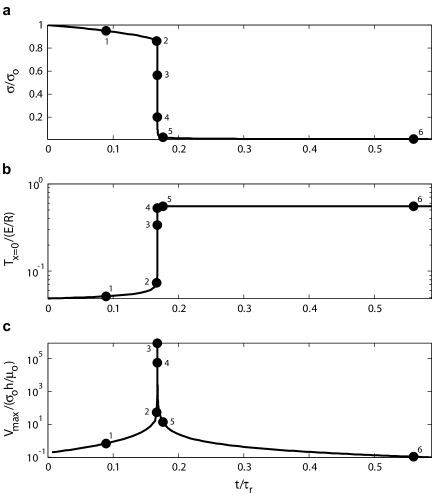
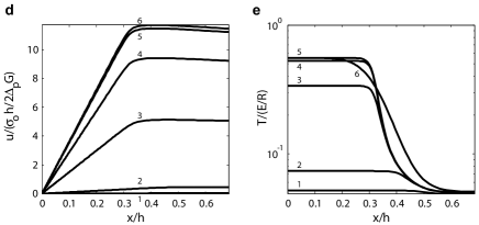
Figure 5: An example of a time evolution of an adiabatic thermal runaway process (see text) corresponding to the location of the dot in Fig. 4. For this particular case $\tilde{T_{0}}\approx 0.0488$, $\tilde{T}_{bg}\approx 0.0476$, $h/L\approx 0.033$, $n=4$, $\tau_{r}/\tau_{d}\approx 0.027$ and $\sigma_{0}/\sigma_{c}\approx 1.83$. Panels (a), (b) and (c) display respectively the shear stress $\sigma$ in units of $\sigma_{0}$, the temperature in the slab center $T_{x=0}$ in units of $E/R$ and the maximum velocity $v_{max}$ in units of $\sigma_{0}h/\mu_{0}$. The two lower panels show a time sequence of spatial distributions in the vicinity of the initially perturbed zone of (d) the displacement $u$ in units of $\sigma_{0}h/2\Delta_{p}G$ and (e) the temperature $T$ in units of $E/R$ (for illustrative purposes we show profiles only for positive $x$). The spatial distributions of $T$ and $u$ are plotted for six different times corresponding to the time markers (black dots) in panels (a)–(c). In all panels the time $t$ is given in units of the relaxation time $\tau_{r}$, and the position $x$ is given in units of the width $h$ of the initially perturbed zone.

As can be seen, the process may be divided into three stages as follows. During the first stage, preceding time marker 2 (i.e., $t<0.17\tau_{r}$), $\sigma(t)$ is seen to decrease nearly linearly with time while the temperature in the slab center $T_{x=0}(t)$ and the maximum velocity $v_{max}(t)$ increase gradually. A corresponding gradual increase in the spatial distributions of the temperature $T$ and the displacement $u$ is noticed in the outer part of the initially perturbed zone having width $h$. However, during the second stage, covered by time markers 2–5 (i.e., in the neighborhood of $t\approx 0.17\tau_{r}$), the shear stress $\sigma$ spontaneously drops to zero and is accompanied by a corresponding explosive rise in the temperature $T_{x=0}$ up to a maximum, whereas one observes an explosive increase in the maximum velocity $v_{max}$ up to a peak value immediately followed by a rapid decrease to a much smaller value again. Moreover, during this short period of time, a dramatic increase in the displacement $u(x,t)$ has occurred in the outer part of the initially perturbed region, while a major, essentially uniform rise in the temperature $T(x,t)$ is observed in the inner part of this region ($0\leq x<0.4h$). This stage, then, represents an extremely rapid thermal runaway process occurring during a time interval much smaller than the thermal diffusion time. The effects of thermal diffusion are therefore seen to be negligible. Finally, during the third stage, succeeding time marker 5 (i.e., $t>0.17\tau_{r}$), $v_{max}$ decreases smoothly towards zero while essentially no further changes in the remaining quantities can be seen. It is worth emphasizing that the rather constant value of the temperature $T_{x=0}$ at this last stage stems from the thermal diffusion time being too large for any noticeable effects of thermal diffusion to be seen within the small time interval exhibited in these plots.

In summary, we observe that thermal runaway processes in the red-colored domain are characterized by a rate of heat production which is much greater than the rate of heat conduction. Accordingly, the runaway process is well approximated as adiabatic and, as was explained in Sec. III.2, the elastic energy in the slab is therefore dissipated essentially uniformly throughout the initially perturbed zone ($|x|\leq h/2$), thus producing a maximum temperature rise $\Delta T_{max}$ which equals the adiabatic temperature rise $\Delta T_{max}^{a}$. Moreover, during the runaway process a dramatic increase in the displacement occurs, which represents the formation of an adiabatic shear band having width of the same order of magnitude as the width $h$ of the initially perturbed zone.

Next, we proceed to analyze the thermal runaway processes occurring in the brown-colored domain, exhibiting much larger temperature rises than $\Delta T_{max}^{a}$. Figure 6 illustrates an example of a thermal runaway process in this domain.

Figure 6: An example of a time evolution of a self-localizing thermal runaway (see text) corresponding to the location of the cross in Fig 4. Here $\tilde{T_{0}}\approx 0.0488$, $\tilde{T}_{bg}\approx 0.0476$, $h/L\approx 0.033$, $n=4$, $\tau_{r}/\tau_{d}\approx 0.006$ and $\sigma_{0}/\sigma_{c}\approx 3.06$. Panels (a)–(e) are organized in the same manner as outlined in the caption of Fig. 5. Note, however, that here the spatial scale in panels (d) and (e) is much smaller than the spatial scale of the corresponding panels (d) and (e) in Fig. 5.

Once again, the time evolution of the process may be divided into three stages; stage one precedes time marker 2 (i.e., $t<0.8\tau_{r}$), stage two is covered by markers 2–5 (i.e., $t\approx 0.8\tau_{r}$), whereas the last stage succeeds time marker 5 (i.e., $t>0.8\tau_{r}$). The initial stage is characterized by a relatively large time interval in which the stress $\sigma$ decreases approximately linearly with time. During the same stage it is seen that the temperature $T_{x=0}$ and the maximum velocity $v_{max}$ increase gradually. There is basically no change in the spatial distributions of the displacement $u(x,t)$ or in the temperature $T(x,t)$. During the second stage, however, a thermal runaway occurs and thus the stress declines spontaneously towards zero. Along with this spontaneous stress drop, one observes an explosive rise in the central temperature up to a maximum followed by a very rapid decrease. It should be emphasized here that, in contrast to what was observed in Fig. 5, the later decrease in $T_{x=0}$ highlights the importance of thermal diffusion for this particular type of thermal runaway. The maximum velocity is seen to accelerate extremely fast up to a peak value immediately followed by an equally fast decrease to a much smaller value again. The dramatic rise in $v_{max}$ as one moves from stage one to stage two is accompanied by a corresponding major rise in $u(x,t)$ and $T(x,t)$. However, the displacement and temperature profiles in this case show strikingly different features as compared to the same profiles obtained in the former case that was shown in Fig. 5. Indeed, in this case, large deformation is seen to occur much closer to the slab center and an extremely non-uniform rise in temperature occurs around the origin. In other words, the strain and temperature profiles continuously localize during the rapid deformation process. Finally, during the third stage, $T_{x=0}$ decreases gradually due to thermal diffusion and the deformation process terminates as $v_{max}$ approaches zero.

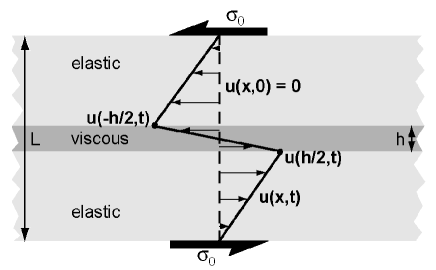
Figure 7: Two rigid elastic plates sliding past one another on a thin viscous layer.

In conclusion, we have seen that thermal runaway processes in the brown-colored domain are characterized by continuous localization of the temperature and strain profiles during deformation, i.e., these runaway processes are spatially “self-localizing”. The elastic energy is thus dissipated in a zone much narrower than the width of the initial perturbation, resulting in maximum temperature rises $\Delta T_{max}$ which are much larger than the maximum adiabatic temperature rises $\Delta T_{max}^{a}$. The self-localization of these runaway processes clearly arises from the effects of thermal diffusion: by diffusion the temperature profile initially acquires a peak in the center where the effect of the positive feedback mechanism accordingly is maximized. The runaway therefore develops faster in the center than in the regions outside and the deformation process finally terminates in a highly localized shear band with a characteristic width much smaller than the width $h$ of the initially perturbed zone.

Finally, we emphasize that the self-localizing failure modes occur at lower values of the shear stress compared to the adiabatic modes. Hence, if the material is subjected to a shear stress large enough to initiate a thermal runaway (i.e., $\sigma\sim\sigma_{c}$), the failure process is expected to be nonadiabatic and to involve a continuous thinning of the developing shear band.

VI Relation between evolution of stress, displacement and temperature rise

Thus far the possibility of catastrophic material failure by spontaneous thermal runaway has been demonstrated. An interesting question yet to be investigated, however, is the relation between stress drop, displacement, shear-band width and temperature rise during runaway, as now discussed.

For this purpose, let us again consider the viscoelastic slab shown in Fig. 1. Assume that the viscosity in the central region $|x|\leq h/2$ is independent of $x$ and much smaller than in the regions outside. In this case the system behaves as if two rigid elastic plates slide past one another on a thin viscous layer (recall, however, that the deforming slab is not far-field driven, but that the outer boundaries $x=\pm L/2$ are clamped as internal deformation occurs). This situation is illustrated in Fig. 7 where we have defined the initial distribution of the displacement field $u(x,t)$ to be $u(x,0)=0$. In accordance with this definition, the shape of the displacement profile is as shown in the figure, and we may define a relative displacement $u_{r}(t)=u(h/2,t)-u(-h/2,t)$ between the boundaries of the viscous layer. For simplicity, we shall study the case when the width of the viscous layer $h$ is much smaller than the system size $L$, i.e., $h/L\ll 1$. Then, denoting the initial stress by $\sigma_{i}$, it is clear that the maximum possible relative displacement is approximately given by

$$u_{r}^{max}\approx\frac{L}{G}\sigma_{0}\,.$$ (55)

We stress here that $\sigma_{0}$ is the initial shear stress in the slab, whereas $u_{r}^{max}$ is the displacement corresponding to the final state for which the slab is completely unloaded. As the rigid plates continue to slide past one another elastic energy stored in the rigid plates is continuously dissipated as heat in the viscous layer. If the sliding process occurs in a time short compared to that for thermal diffusion, the energy equation for this layer may be written

$$C\frac{\partial T}{\partial t}=\sigma(t)\frac{\partial\gamma}{\partial t}\,,$$ (56)

where $\gamma$ denotes the strain inside the viscous central region and the term on the r.h.s. of the equation is the work dissipated during irreversible viscous flow. It was seen in the examples of thermal runaway events in the previous section that the shear stress does not remain constant during deformation, but drops spontaneously towards zero. Hence, $\sigma(t)$ is a strongly varying function of time and as a consequence Eq. (56) cannot be integrated over time directly. This apparent complication may be circumvented, however, by instead expressing both $\sigma$ and $\gamma$ as functions of the displacement. In correspondence with the adiabatic assumption made here, the temperature rise within the viscous layer will be uniform. Since the viscosity then is a function of both a uniform temperature and shear stress, it follows that the viscosity and accordingly the strain within the viscous layer is uniform. Then, from inspection of Fig. 7, it is seen that the uniform strain can be expressed as a function of the relative displacement $u_{r}$ according to the relation

$$\gamma(t)=\frac{u_{r}(t)}{h}\,,$$ (57)

from which we obtain the strain rate

$$\frac{d\gamma}{dt}=\frac{1}{h}\frac{du_{r}(t)}{dt}\,.$$ (58)

Similarly, in the limit $L>>h$ and because the outer rigid plates are purely elastic, it can be gleaned from Fig. 7 that the stress approximately is given by

$$\sigma(t)\approx\sigma_{0}-G\frac{u_{r}(t)}{L}\,.$$ (59)

Substituting these expressions for $d\gamma/dt$ and $\sigma(t)$ in Eq. (56) and using that $u_{r}(t)(du_{r}/dt)=1/2(du_{r}^{2}/dt)$, the energy equation takes the form

$$C\frac{dT}{dt}=\frac{d}{dt}\left[\left(\sigma_{0}-\frac{G}{2L}u_{r}(t)\right)\frac{u_{r}(t)}{h}\right]\,.$$ (60)

Next, it follows from Eq. (59) that $(G/2L)u_{r}(t)=\frac{1}{2}(\sigma_{0}-\sigma(t))$, and the energy equation may thus be written

$$C\frac{dT}{dt}=\frac{d}{dt}\left[\frac{1}{2}\left(\sigma_{0}+\sigma(t)\right)\frac{u_{r}(t)}{h}\right]\,,$$ (61)

thereby eliminating $G/L$ from the equation. The desired relation between dynamic quantities can now be obtained by direct integration of the energy equation with respect to time. If the deformation process terminates at some final time $t_{f}$, then upon integrating from $t=0$ to $t_{f}$, we find

$$C\Delta T^{f}=\frac{(\sigma_{0}+\sigma_{f})}{2}\frac{u_{r}^{f}}{h}\,.$$ (62)

Here $\sigma_{f}=\sigma(t_{f})$, $\Delta T^{f}=T(x,t_{f})-T(x,0)$ and $u_{r}^{f}=u_{r}(t_{f})$. Not surprisingly, Eq. (62) shows that to correctly account for decrease in shear stress during deformation, one should use the average of the initial and final shear stress in calculating the work done by the rigid plates on the viscous layer.

The relation between dynamic quantities in Eq. (62) was obtained under the assumption of adiabatic conditions. Yet, it was clarified in the previous section that thermal runaway processes are greatly affected by thermal diffusion and therefore not truly adiabatic. As a consequence shear was seen to localize to a region of width much smaller than the width $h$ of the initially perturbed region. It is therefore of interest to evaluate the accuracy of Eq. (62) for the more general case, including self-localizing runaway processes, by numerical methods. For this reason proper definitions of the quantities entering Eq. (62), valid also for nonadiabatic processes, are needed.

Figure 6 shows that the first stage of stress relaxation does not contribute notably to deformation. We define the initial shear stress $\sigma_{i}$ associated with the process of shear-band formation to be the stress at the instant $t_{i}$ at which the curvature of the temporal stress curve $d^{2}\sigma/dt^{2}$ first becomes negative. Thus $\sigma_{i}$ is the shear stress in the slab right at the onset of thermal runaway. The final stress, $\sigma_{f}$, is defined as the stress corresponding to the instant $t_{f}$ at which $d^{2}\sigma/dt^{2}$ exhibits a maximum. $\sigma_{f}$ is thus the shear stress in the slab right at the instant at which the thermal runaway process terminates. For illustration, $\sigma_{i}$ and $\sigma_{f}$ are the stresses corresponding to time markers 2 and 5 in Fig. 6(a), respectively. Next, in order to define the shear band properly, we must identify the point in the displacement profile where a sharp transition from very large strain to small strain occurs (for example, in the displacement profile corresponding to time marker 6 in Fig. 6(d), this sharp transition occurs at the position $x/h\approx 0.01$). For this reason, we must analyze the second derivative of the displacement profile $\partial^{2}u/\partial x^{2}$ at the instant of time when the runaway process terminates (essentially no further deformation occurs for later times). We define the shear band to be the region $|x|\leq w/2$, where $x=w/2$ corresponds to the position at which $\partial^{2}u/\partial x^{2}$ becomes a minimum (by symmetry $\partial^{2}u/\partial x^{2}$ becomes a maximum at $x=-w/2$). The final relative displacement across the shear band is then given by $u_{r}^{f}=u(w/2,t_{f})-u(-w/2,t_{f})$. In our numerical calculations we replace the quantities $\sigma_{0}$ and $h$ in Eq. (62) by $\sigma_{i}$ and $w$, respectively. Lastly, the temperature rise $\Delta T^{f}$ in Eq. (62) is now taken to be the maximum temperature rise $\Delta T_{max}$ occurring in the center of the slab.

With all the quantities properly defined, and since the controlling variables for onset of thermal runaway have been identified, it is now possible to investigate the robustness of Eq. (62) by numerical analysis. Numerical calculations of the quantities entering Eq. (62) versus the controlling physical parameters $\sigma_{0}/\sigma_{c}$ and $\tau_{r}/\tau_{d}$, where the controlling parameters are varied over the same range as in Fig. 4, show that

$$1\lesssim\frac{2wC\Delta T_{max}}{\left(\sigma_{i}+\sigma_{f}\right)u_{r}^{f}}\lesssim 2\,.$$ (63)

Hence, according to our model, the simple relation in (62) is applicable even to nonadiabatic situations leading to self-localizing processes.

VII Discussion and conclusions

The mechanism of spontaneous thermal runaway in viscoelastic solids has been analyzed within the framework of a highly simplified one-dimensional continuum model. As a first approximation the model is only intended to contain the most essential physics governing the thermal runaway phenomenon and certainly neglects many important effects encountered in the more complicated experimental situations.

Among the most crucial simplifications made in the present model is perhaps our neglect of significant changes of material properties that may result from the very large temperature rises associated with the runaway instability. The model does not include corrections due to effects of melting, although melting of the material near the shear band may be possible. Also, the influence of melting on shear-band formation could potentially increase the rate of deformation even further and cause propagation of elastic waves, which would then require consideration of inertial effects. For these reasons the calculations made within the present model are strictly valid only until these changes take place, and the model may therefore be assumed to reproduce only qualitatively the correct deformation behavior during the later stages of the thermal runaway process. However, the inertia becomes significant only after the onset of localization and/or thermal runaway and hence does not affect the conclusions of our study. This statement was also checked by additional numerical studies based on the full system of equations which include the inertial terms.

Our approach has thus been to investigate the simplest possible model which still has some expectation of representing a real physical situation reasonably well. Although the ideal character of the model should not be ignored, it allows for a quantitative treatment of the deformation problem that hopefully provides valuable information about the behavior of the thermal runaway failure mechanism.

A basis for the theory is the assumption that the temperature dependence of the material’s viscosity can be described approximately by an Arrhenius expression, and that it generally has a nonlinear dependence on the shear stress. This represents a simple model accounting for thermally activated transitions in the solid, believed to be responsible for nonelastic behavior below the yield stress. As a consequence, thermal runaway instability may occur due to shear heating-induced thermal softening of the material.

In order to determine the conditions necessary for thermal runaway to occur a theoretical analysis was carried out. Neglecting the effect of thermal diffusion, i.e., assuming adiabatic conditions during deformation, approximate analytical solutions supposed to be valid for the early stages of time evolutions of temperature and shear stress were found. For this case it was shown that the system becomes unstable against shear banding due to spontaneous thermal runaway if the initial shear stress $\sigma_{0}$ becomes larger than a critical stress $\sigma_{c}$ (Eq. (20)). To investigate the effects of thermal diffusion on the instability conditions, we subsequently performed a linear analysis using rather rough approximations of the complete system of equations. The stability condition obtained within the adiabatic approximation was then modified to include an additional controlling combination of physical parameters, namely the ratio of the relaxation time $\tau_{r}$ to the thermal diffusion time $\tau_{d}$. According to this analysis $\sigma_{c}$ still provides a good estimate for the critical stress above which spontaneous thermal runaway occurs as long as $\tau_{r}/\tau_{d}<1$. However, when $\tau_{r}/\tau_{d}\gg 1$, the rate of relaxation or creep in the material is very small compared to the process of thermal diffusion, and the stress required for thermal runaway to occur in this case is therefore much larger. These results were independently verified by finite amplitude numerical analysis as demonstrated by a series of contour plots of the maximum temperature rise $\Delta T_{max}$ (Fig. 3). Hence we conclude that initiation of spontaneous thermal runaway is controlled by the two combinations of parameters $\sigma_{0}/\sigma_{c}$ and $\tau_{r}/\tau_{d}$ only.

Numerical investigation of the maximum temperature rises and displacement profiles during thermal runaway instabilities revealed two potential types of thermal runaway processes having distinctly different characters. The first, occurring under near adiabatic conditions, is characterized by essentially uniform temperature rise and strain inside the perturbed zone and is therefore referred to as adiabatic thermal runaway. The second, occurring under nonadiabatic conditions, is characterized by continuous localization of the temperature and strain profiles during deformation and is accordingly referred to as self-localizing thermal runaway. However, the self-localizing failure modes occur at lower values of the shear stress compared to the adiabatic modes. In materials subjected to increasing loads the actual failure process is therefore expected to be nonadiabatic. Thus, if the shear stress in the material exceeds a critical value of the order of $\sigma_{c}$, the material starts to internally disintegrate by unloading the elastic energy stored in the bulk of the medium through accelerated creep along a continuously narrowing band. Since creep is a thermally activated process, this rapid increase in creep is achieved by local rise in temperature. In turn, the accelerated creep prevents the material from local cooling due to thermal conduction. This opens for the possibility that some materials become unstable against macroscopic perturbations (that localize extremely while developing) before reaching the theoretical shear strength limit at which the material would break locally, i.e., at the lattice scale. In this way the material may fail by ductile deformation at scales much smaller than the deforming sample size, and notably at scales much smaller than the characteristic width of an initial thermal perturbation, but which still are orders of magnitude larger than interatomic spacing.

Finally, a quantitative relation between evolution of stress, deformation and temperature rise was obtained for adiabatic shear banding processes by analytical methods. Numerical calculations of self-localizing thermal runaway processes within our simple viscoelastic model have been carried out, showing that the same relation is valid also for this particular case. In order to establish the robustness of Eq. (62), however, it would be instructive to compare this relation to the results of improved model calculations of the later stages of thermal runaway processes taking into account important changes in material properties as commented upon above.

Recent studies Torgeir08 ; pseudothac showed that the theory developed here and in Ref. [BP, ] is applicable to explain the generation of intermediate-depth earthquakes. In contrast to this study in which we consider infinitesimal perturbations ($\Delta_{p}\approx 1$ and $T_{0}\approx T_{bg}$), John et al. pseudothac considers large amplitude finite perturbations of the system caused by water influence on rheological properties of rocks subjected to differential stresses. Even though the finite amplitude perturbations distort the data collapse (such as presented in Fig. 3), the representation of results as function of the two combinations of parameters $\sigma_{0}/\sigma_{c}$ and $\tau_{r}/\tau_{d}$ was proved to be useful. Using laboratory derived properties of diabase, the typical representative of lower crust rocks, John et al. [pseudothac, ] show that the self-localizing thermal runaway can be considered as a potential mechanism for deep earthquakes.

A thorough, quantitative comparison of the theory presented here with experiments on bulk metallic glasses and polymers at various loading conditions and temperatures is outside the scope of the present discussion. Nevertheless, a very rough estimate of the ratios $\sigma_{0}/\sigma_{c}$ and $\tau_{r}/\tau_{d}$ for bulk metallic glasses is possible. For bulk metallic glasses, typical values are $C$=1.6$\times 10^{6}$ J m^-3K^-1 (Ref. [Lewandowski, ]), $G$=34 GPa (Ref.  [JohnsonSamwer, ]), $E$= 100–400 kJ mole^-1 (Ref. [Wang, ; Chen, ]). Assuming a temperature $T_{bg}\approx 620$ K and infinitely-small amplitude of the perturbation, i.e., $\Delta_{p}\approx 1$, we obtain $\sigma_{c}$ = 0.8–2 GPa. Our study shows, however, that the critical value of the stress $\sigma_{0}$ needed to initiate self-localizing thermal runaway may differ significantly from $\sigma_{c}$ if the ratio $\tau_{r}/\tau_{d}$ is large. The estimate of this ratio is much less certain. Only the thermal diffusivity $\kappa$ has a well-established value of 3$\times 10^{-6}$ m²s^-1 (Ref. [Lewandowski, ]). From Ref. [Johnson, ] the viscosity $\mu_{0}$ at this temperature is inferred to be approximately 10¹¹–10¹² Pa$\cdot$s. The characteristic width $h$ of the initial perturbation, representing a macroscopic perturbation in the material, is highly uncertain but a lower bound may be estimated. Experimental observations Lewandowski of the width $w$ of the zone affected by deformation around shear bands give $w\approx 1$ $\mu$m. Because of the self-localizing nature of the deformation (Fig. 5c), we expect that $h\gg w$, and hence we assume $h$ = 10 $\mu$m - 10 mm (limited by the typical sample size). These very rough estimates give a value for the dimensionless ratio $\tau_{r}/\tau_{d}$ ranging from 10^-2 to 10⁵ and the critical value of $\sigma_{0}$ necessary for self-localizing thermal runaway to occur may be expected to be close to the critical stress $\sigma_{c}$. It should be noted that our estimate of $\sigma_{0}\approx\sigma_{c}\approx$ 0.8-2 GPa represents the upper limit of critical stress in the system. Modifications of our idealized model setup by e.g. increasing the intensity of the initial perturbation (decreasing $\Delta_{p}$) and accounting for the effect of dynamically building up the shear stress in the system would significantly decrease the stress required to initiate instability pseudothac . Without detailed analysis of particular cases, a quantitative comparison of our theory to experimental results on bulk metallic glasses is, at present, somewhat difficult as the above estimate of the ratio $\tau_{r}/\tau_{d}$ clearly is insufficiently constrained. Explicit studies invoking appropriate constitutive behavior should be undertaken; for example, it might be more realistic using a Vogel-Fulcher-Tamman or Cohen-Grest CohenGrest dependence of viscosity on temperature instead of the Arrhenius dependence employed here. However, the self-localizing thermal runaway mechanism appears to be compatible with current experimental data and should, in our opinion, be considered as a potential mechanism governing instabilities also in materials such as bulk metallic glasses and glassy polymers.

The study pseudothac also demonstrated that the theory may be applicable to the system described not only for thermal, but also for rheological perturbations such as variations of activation energy of creep $E$ and/or pre-exponential constant $A$. The rheological model of the system (Eq. 3) may also be extended to include low temperature plasticity (Peierl s plasticity Schulson ).

- (1) J. Lu and K. Ravi-Chandar, Int. J. Solids Struct. 36, 391 (1999).
- (2) J.C.M. Li, Polym. Eng. Sci. 24, 750 (1984).
- (3) A. Cross and R. N. Haward, J. Polym. Sci., Polym. Phys. Ed. 11, 2423 (1973).
- (4) A.L. Greer, Science 267, 1947 (1995).
- (5) W.J. Wright, R.B. Schwarz, and W.D. Nix, Mater. Sci. Eng. A 319–321, 229 (2001).
- (6) J.J. Lewandowski and A.L. Greer, Nat. Mater. 5, 15 (2006)
- (7) C.C. Hays, C.P. Kim, and W.L. Johnson, Phys. Rev. Lett. 84, 2901 (2000).
- (8) C.E. Renshaw and E.M. Schulson, J. Geophys. Res. 109, B09207 (2004).
- (9) M. Obata and S. Karato, Tectonophysics 242, 313 (1995).
- (10) D.A. Wiens, Phys. Earth Planet. Int. 127, 145 (2001).
- (11) P.J. Miller, C.S. Coffey, and V.F. DeVost, J. Appl. Phys. 59, 913 (1986).
- (12) T. W. Wright, The Physics and Mathematics of Adiabatic Shear Bands (Cambridge University Press, Cambridge, UK, 2002).
- (13) C.E. Renshaw and E.M. Schulson, Earth Planet. Sci. Lett. 258, 307 (2007).
- (14) C.A. Pampillo, J. Mater. Sci. 10, 1194 (1975).
- (15) E. Pekarskaya, C.P. Kim, and W.L. Johnson, J. Mater. Res. 16, 2513 (2001).
- (16) V.Z. Bengus et al., J. Mater. Sci. 35, 4449 (2000).
- (17) T.B. Andersen and H. Austrheim, Earth Planet. Sci. Lett. 242, 58 (2006).
- (18) H. Austrheim and T.M. Boundy, Science 265, 82 (1994).
- (19) T. John and V. Schenk, Geology 34, 557 (2006).
- (20) J. Frenkel, Z. Phys. 37, 572 (1926).
- (21) Y. Zhang and A.L. Greer, Appl. Phys. Lett. 89, 071907 (2006).
- (22) J.A. Åström, H.J. Herrmann and J. Timonen, Phys. Rev. Lett. 84, 638 (2000).
- (23) B. Francois, Frédéric Lacombe and H.J. Herrmann, Phys. Rev. E 65, 031311 (2002).
- (24) A. Molinari and R.J. Clifton, J. Appl. Mech. 54, 806 (1987).
- (25) W.L. Johnson, J. Lu and M.D. Demetriou, Intermetallics 10, 1039 (2002).
- (26) C.A. Schuh, T.C. Hufnagel and U. Ramamurty, Acta Mater. 55, 4067 (2007).
- (27) F. Spaepen, Acta Metall. 25, 407 (1977).
- (28) A.S. Argon, Acta Metall. 27, 47 (1979).
- (29) A.S. Argon and L.T. Shi, Acta Metall. 31, 499 (1983).
- (30) M.L. Falk and J.S. Langer, Phys. Rev. E 57, 7192 (1998).
- (31) A.L. Greer, Materials Today 12, 14 (2009).
- (32) J.S. Langer, Phys. Rev. E 64, 011504 (2001).
- (33) M.L. Manning, J.S. Langer and J.M. Carlson, Phys. Rev. E 76, 056106 (2007).
- (34) D.T. Griggs and D.W. Baker, Properties of Matter under Unusual Conditions (Wiley, New York, 1968).
- (35) M. Ogawa, J. Geophys. Res. 92, 13801 (1987).
- (36) S. Braeck and Y.Y. Podladchikov, Phys. Rev. Lett. 98, 095504 (2007).
- (37) E.E. Zhurkin, T. Van Hoof, and M. Hou, Phys. Rev. B 75, 224102 (2007).
- (38) L.E. Malvern, Introduction to the Mechanics of a Continuous Medium (Prentice-Hall, Englewood Cliffs, N.J., 1969).
- (39) B.J.P. Kaus and Y.Y. Podladchikov, J. Geophys. Res. 111, B04412 (2006).
- (40) T.B. Andersen, K. Mair, H.O. Austrheim, Y.Y. Podladchikov, J.C. Vrijmoed, Geology 36, 995 (2008).
- (41) T. John, S. Medvedev, L. Rüpke, T.B. Andersen Y.Y. Podladchikov, and H. Austrheim, Nature Geoscience 2, 137 (2009).
- (42) W. L. Johnson and K. Samwer, Phys. Rev. Lett. 95, 195501 (2005).
- (43) Q.Wang, J. Lu, F. J. Gu, H. Xu, and Y. D. Dong, J. Phys. D 39, 2851 (2006).
- (44) H. S. Chen, Rep. Prog. Phys. 43, 353 (1980).
- (45) M.H. Cohen and G.S. Grest, Phys. Rev. B 20, 1077 (1979).