Friedel oscillations induced surface magnetic anisotropy

Abstract

We present detailed numerical studies of the magnetic anisotropy energy of a magnetic impurity near the surface of metallic hosts (Au and Cu), that we describe in terms of a realistic tight-binding surface Green’s function technique. We study the case when spin-orbit coupling originates from the d-band of the host material and we also investigate the case of a strong local spin-orbit coupling on the impurity itself. The splitting of the impurity’s spin-states is calculated to leading order in the exchange interaction between the impurity and the host atoms using a diagrammatic Green’s function technique. The magnetic anisotropy constant is an oscillating function of the separation $d$ from the surface: it asymptotically decays as $\sim 1/d^{2}$ and its oscillation period is determined by the extremal vectors of the host’s Fermi Surface. Our results clearly show that the host-induced magnetic anisotropy energy is by several orders of magnitude smaller than the anisotropy induced by the local mechanism, which provides sufficiently large anisotropy values to explain the size dependence of the Kondo resistance observed experimentally.

I Introduction

It is by now more than fifteen years ago that a surprising suppression of the Kondo effect in thin films and wires of dilute magnetic alloys has been observed.exp1 ; exp2 ; exp3 ; exp4 A few years after the first experiments, Újsághy et al. proposed that the most likely explanation of the experimental observations is a spin-orbit coupling induced magnetic anisotropy in the vicinity of the surface of the films: In the presence of a surface, spin-orbit (SO) coupling gives rise to a level splitting of the impurity spin, and thus blocks the spin-flip processes responsible for the Kondo effect orsi1 ; orsi2 ; orsi3 . Indeed, later experiments seemed to be in agreement with this simple scenario and confirmed the predictions that follow from it.exp5 Fitting the experimental data for a $Au(Fe)$ film, Újsághy et al.orsi1 estimated the width of the ‘dead layer’, $L_{c}$, where the splitting is larger or comparable to the Kondo temperature, $T_{K}=0.3K\simeq 0.03$ meV, and obtained $L_{c}\simeq 180$ Å.

To explain the unexpectedly large width of the dead layer, Újsághy et al. also proposed a model to describe surface-anisotropy, which we shall refer to as the host spin-orbit coupling (HSO) model. In this model an impurity with a half-filled $d$-shell and spin $S=5/2$ is immersed in a host metal, where conduction electrons experience SO scattering through hybridizing with low-lying valence $d$-orbitals of the host material.orsi1 ; orsi2 ; orsi3 These calculations have been revised recently in Ref. orsi4, . This HSO mechanism does not lead to the splitting of the six-fold degenerate spin state of the impurity, when placed in a bulk host with high (cubic or continuous rotational) symmetry. However, the presence of the surface induces an anisotropy term,

$$H^{\rm HSO}_{\rm anis}=K(d)\left({\bf n}\,{\bf S}\right)^{2}\;,$$ (1)

where ${\bf n}$ is the normal vector of the surface, ${\bf S}$ is the spin-operator, and $K(d)$ denotes the magnetic anisotropy constant at a distance $d$ from the surface. The anisotropy constant $K(d)$ can be estimated in a simple free electron model, by treating the spin-orbit coupling, $\xi$, and the exchange coupling, $J$, perturbatively. This calculation leads to the asymptotic form,orsi4

$$K(d)=A(k_{F})J^{2}\xi^{2}\frac{\sin(2k_{F}d)}{d^{3}}\;,$$ (2)

where $k_{F}$ is the Fermi wavenumber.footnote1 Unfortunately, the constant $A(k_{F})$ contains some cut-off parameters, which make the above formula less predictive for the experiments. However, ab initio calculationsSG:prl97 indicated that this bulk mechanism is too weak to explain the experimental findings.

Recently, however, a rather different mechanism has been proposed to produce a magnetic anisotropy in the vicinity of a surface.SZG:prl06 This mechanism, which we shall refer to as local spin-orbit coupling (LSO) mechanism, assumes only a strong local SO coupling on the impurity’s $d$-level. The basic observation leading to this mechanism is that, for partially filled $d$-shells, spin-states have also a large orbital content. Therefore, spin states couple very strongly to Friedel oscillations in the vicinity of a surface: electrons on the deep $d$-levels can lower their energy by hybridizing with the conduction electrons through virtual fluctuations. The corresponding anisotropy appears already to first order in the exchange coupling $J$ and decays as $\sim 1/d^{2}$. In the specific case of an impurity with a $d^{1}$ configuration, the corresponding $J_{3/2}$ ground state multiplet is split by the presence of the surface asSZG:prl06

$$H^{\rm LSO}_{\rm anis}=K(d)\left({\bf n}\,{\bf J}\right)^{2}\;,$$ (3)

where ${\bf J}$ stands for the total angular momentum operators, and $K(d)\sim J\sin(Q_{F}d)/d^{2}$, with $Q_{F}$ being the length of an extremal vector of the Fermi Surface (FS). As shown in Ref. SZG:prl06, the anisotropy can take the desired value of about a few tenths of meV even beyond 100 Å from the surface.

Although the second (local) mechanism is expected to be dominant for impurities with partially filled (not half-filled) $d$-shells, in Ref. SZG:prl06, only a toy model, namely, a single-band metal on a simple cubic lattice, has been considered. For a quantitative comparison, however, and to decide, which mechanism is responsible for the surface-induced anisotropy, more realistic lattice and band structures should be used. The aim of the present work is to provide such a qualitative and quantitative comparison of the two mechanisms described above. For this purpose, we shall embed the impurity into an fcc lattice, and employ realistic tight-binding surface Green’s function methodssgfm to describe the conduction and valence electrons of the host material. This method allows for a numerically exact treatment of the surface, and also incorporates the SO coupling non-perturbatively.

To describe the magnetic impurity, we shall integrate out virtual charge fluctuations on the $d$-level of the magnetic impurity, and construct realistic spin models, which take into account the specific magnetic and crystal field structure of the impurity.CoxZawa

We shall then study the surface-induced anisotropy within both models, and derive explicit expressions for the anisotropy constants in terms of the local density of states around the magnetic impurity. Analyzing the behavior of $K(d)$ in the asymptotic regime, we find that the oscillations of $K(d)$ are related to the extremal vectors of the Fermi surface. For the case of Au and Cu host metals, we perform numerical calculations of the anisotropy constants as based on the asymptotic formulas and the oscillation periods are directly identified from the numerically computed Fermi surface. In the case of the local SO model, we are also able to confirm numerically the validity of the asymptotic expressions. Our results support the priority of the local SO mechanism.

II Short review of the theoretical approach

Before we present our results, let us to some extent outline the theoretical methods we use. As mentioned in the introduction, in our approach we describe the host material within a tight binding Green’s function formalism. The interaction between the magnetic impurity and the host, on the other hand, is described in terms of an effective interaction, which we construct by combining group theoretical methods with many-body techniques. Once this effective exchange interaction Hamiltonian at hand, we can use relatively standard field theoretical toolspseudofermion to do perturbation theory in the exchange coupling, and determine the surface-induced anisotropy.

II.1 The Green’s function of the host

In this paper, we shall study surfaces of ordered non-magnetic hosts, like the (001) surface of Au or Cu. In this case, the Hamiltonian of the host can be written as,

$$\mathring{H}_{\lambda\sigma,\lambda^{\prime}\sigma^{\prime}}^{pn,p^{\prime}n^{\prime}} = \left(\varepsilon_{\lambda}\,\delta_{\lambda\lambda^{\prime}}\delta_{\sigma\sigma^{\prime}}+\xi\left(\mbox{\boldmath$\ell$}\cdot{\mathbf{s}}\right)_{\lambda\sigma,\lambda^{\prime}\sigma^{\prime}}\right)\delta_{pp^{\prime}}\delta_{nn^{\prime}}+$$ (4)

$$+ V_{\lambda,\lambda^{\prime}}^{pn,p^{\prime}n^{\prime}}\,\delta_{\sigma\sigma^{\prime}}\quad,$$

where $p$, $p^{\prime}$ denote atomic layers normal to the surface, $n$, $n^{\prime}$ label atomic sites within the layers, while $\lambda$, $\lambda^{\prime}$ denote the canonical $spd$ orbitals centered at the lattice positions and $\sigma$, $\sigma^{\prime}$ are spin indices. In Eq. (4), we replaced all the parameters by their bulk values, i.e., we neglected the dependence of the on-site energies, $\varepsilon_{\lambda}$ and the SO parameter, $\xi$, on the layer depth $p$. The hopping matrix elements, $V_{\lambda,\lambda^{\prime}}^{pn,p^{\prime}n^{\prime}}$ are confined to first and next-nearest neighbors, and their layer-dependence is also neglected. These approximations lead certainly to some errors in the calculated electronic structure very close to the surface, however, they are expected to have no serious consequences in the asymptotic regime, which is the subject of our interest. By the same token, in the vacuum (i.e., $p\leq 0$) the on-site energies are taken to be infinity. This simplifies somewhat our calculations, since only layers $p\geq 1$, forming thus a semi-infinite system, need to be considered in the evaluation of the Green’s function.

The Hamiltonian Eq. (4) can be recast into a matrix in the spin and orbital labels,

$$\underline{\mathring{H}}^{pn,p^{\prime}n^{\prime}}=\left\{\mathring{H}_{\lambda\sigma,\lambda^{\prime}\sigma^{\prime}}^{pn,p^{\prime}n^{\prime}}\right\}\;.$$ (5)

Since our system is translational invariant within the layers, we can also define the Fourier transform of the Hamiltonian matrix, $\underline{\mathring{H}}^{pp^{\prime}}({\bf k})$, and introduce the ’semi-infinite’ matrix,

$$\mathring{\cal H}({\bf k})=\left\{\underline{\mathring{H}}^{pp^{\prime}}({\bf k})\right\}_{p,p^{\prime}\geq 1}\;.$$ (6)

The resolvent or Green’s function matrix is then given as usual

$$\mathring{\cal G}(z,{\bf k})=\left(z-\mathring{\cal H}({\bf k})\right)^{-1}\;,$$ (7)

with $z$ a complex number (energy).

To perform the matrix inversion in Eq. (7), we used the surface Green’s function technique,sgfm which is an efficient and, in principle, exact tool to compute the Green’s function. Most importantly, the computational time of this method scales linearly with the number of layers, for which the Green’s function is evaluated. The real-space representation of the Green’s function can then be obtained by performing the following Brillouin zone (BZ) integral,

$$\underline{\mathring{G}}^{pn,p^{\prime}n^{\prime}}(z)=\frac{1}{\Omega_{BZ}}\int d^{2}k\,\underline{\mathring{G}}^{pp^{\prime}}(z,{\bf k})\,e^{-i{\bf k}({\bf T}_{n^{\prime}}-{\bf T}_{n})}\;,$$ (8)

where $\Omega_{BZ}$ is the volume of the 2-dimensional Brillouin zone, and the translation vector ${\bf T}_{n}$ is related to the position of atom $n$ in layer $p$ as ${\bf R}_{pn}={\bf C}_{p}+{\bf T}_{n}$, with ${\bf C}_{p}$ a layer-dependent reference position.

The host-Hamiltonian, Eq.(4), must be slightly modified in the presence of a magnetic impurity. In this case, the hopping of the conduction electrons to the impurity’s $d$-orbitals should be excluded, since these processes involve charge fluctuations at the magnetic impurity site, which will be incorporated in the effective exchange interaction (see next section). The simplest way to account for this constraint is to shift the on-site $d$-state energies of the impurity, $\varepsilon^{i}_{\lambda}$, far below the valence band, and add the following term to the Hamiltonian,

$$\Delta H_{\lambda\sigma,\lambda^{\prime}\sigma^{\prime}}^{(q)pn,p^{\prime}n^{\prime}}=\left(\varepsilon^{i}_{\lambda}-\varepsilon_{\lambda}\right)\delta_{pq}\,\delta_{p^{\prime}q}\,\delta_{n0}\,\delta_{n^{\prime}0}\,\delta_{\lambda,\lambda^{\prime}}\,\delta_{\sigma\sigma^{\prime}}\;,$$ (9)

where the impurity is at site $n=0$ and in layer $q$.

To describe the spin dynamics, we do not need to evaluate the full Green’s function: We need its value only for a small cluster of sites, ${\cal C}^{(q)}$, consisting of nearest neighbor atoms around the impurity and the impurity itself. Fortunately, since $\Delta H$ is also local, this restricted Green’s function,

$$\underline{\underline{G}}^{(q)}(z)=\left\{\underline{G}^{pn,p^{\prime}n^{\prime}}\right\}_{{\cal C}^{(q)}}\;,$$ (10)

can be evaluated as

$$\underline{\underline{G}}^{(q)}(z)=\left(\underline{\underline{I}}-\underline{\underline{\mathring{G}}}^{(q)}(z)\,\Delta\underline{\underline{H}}^{(q)}\right)^{-1}\underline{\underline{\mathring{G}}}^{(q)}(z)\;,$$ (11)

where $\underline{\underline{I}}$ is the unit matrix, and the matrix elements of $\underline{\underline{\mathring{G}}}^{(q)}(z)$ and $\Delta\underline{\underline{H}}^{(q)}$ are defined in Eqs. (8) and (9), respectively. Finally, the spectral function matrix on this cluster is defined as

$$\underline{\underline{\varrho}}^{(q)}(\varepsilon)=-\frac{1}{2\pi i}\lim_{\delta\rightarrow+0}\left(\underline{\underline{G}}^{(q)}(\varepsilon+i\delta)-\underline{\underline{G}}^{(q)}(\varepsilon-i\delta)\right)\;.$$ (12)

As shown in the following subsections, the matrix elements of this spectral function matrix are directly related to the magnetic anisotropy.

II.2 Host spin-orbit model of the magnetic anisotropy

As in Refs. orsi1, ; orsi2, ; orsi3, ; orsi4, let us first consider a spin $S=5/2$ impurity with a half-filled $d$-shell. In this case, we can neglect the SO interaction on the magnetic ion, and the bulk SO interaction is the primary source of the surface-induced anisotropy.

$|1\rangle$	$D_{xz}=\frac{1}{2}\left(s_{{\bf x}{\bf z}}+s_{\bar{\bf x}\bar{\bf z}}-s_{{\bf x}\bar{\bf z}}-s_{\bar{\bf x}{\bf z}}\right)$
$|2\rangle$	$D_{yz}=\frac{1}{2}\left(s_{{\bf y}{\bf z}}+s_{\bar{\bf y}\bar{\bf z}}-s_{{\bf y}\bar{\bf z}}-s_{\bar{\bf y}{\bf z}}\right)$
$|3\rangle$	$D_{xy}=\frac{1}{2}\left(s_{{\bf x}{\bf y}}+s_{\bar{\bf x}\bar{\bf y}}-s_{{\bf x}\bar{\bf y}}-s_{\bar{\bf x}{\bf y}}\right)$
$|4\rangle$	$D_{x^{2}-y^{2}}=\frac{1}{2\sqrt{2}}\left(s_{{\bf y}{\bf z}}+s_{\bar{\bf y}\bar{\bf z}}+s_{{\bf y}\bar{\bf z}}+s_{\bar{\bf y}{\bf z}}-s_{{\bf x}{\bf z}}-s_{\bar{\bf x}\bar{\bf z}}-s_{{\bf x}\bar{\bf z}}-s_{\bar{\bf x}{\bf z}}\right)$
$|5\rangle$ nnn	$D_{2z^{2}-x^{2}-y^{2}}=\frac{1}{2\sqrt{6}}\left(2s_{{\bf x}{\bf y}}+2s_{\bar{\bf x}\bar{\bf y}}+2s_{{\bf x}\bar{\bf y}}+2s_{\bar{\bf x}{\bf y}}-s_{{\bf y}{\bf z}}-s_{\bar{\bf y}\bar{\bf z}}-s_{{\bf y}\bar{\bf z}}-s_{\bar{\bf y}{\bf z}}-s_{{\bf x}{\bf z}}-s_{\bar{\bf x}\bar{\bf z}}-s_{{\bf x}\bar{\bf z}}-s_{\bar{\bf x}{\bf z}}\right)$

Table 1: Combinations of $s$-orbitals centered at the 12 neighbor sites around an impurity having the symmetry of atomic $d$ orbitals.

To construct the effective interaction between the host electrons and the magnetic impurity, one can safely assume that the deep $d$-levels of the magnetic impurity hybridize only with the $s$-orbitals of the neighboring host atoms. However, by symmetry, the deep $d$-levels can hybridize only with appropriate linear combinations of these $s$-orbitals, $\alpha\in\{x^{2}-y^{2},2z^{2}-x^{2}-y^{2},xy,xz,yz\}$. In case of an fcc lattice, e.g., we have 12 nearest neighbor $s$-orbitals, which can be labeled by $s_{{\bf x}{\bf y}}$, $s_{\bar{\bf x}\bar{\bf y}}$, $s_{{\bf x}\bar{\bf y}}$, $s_{\bar{\bf x}{\bf y}}$, $\dots$, $s_{{\bf y}\bar{\bf z}}$, $s_{\bar{\bf y}{\bf z}}$, the subscripts ${\bf x}{\bf y}$ and $\bar{\bf x}\bar{\bf y}$ referring to neighboring sites at the positions $a(\frac{\footnotesize{1}}{\footnotesize{2}},\frac{\footnotesize{1}}{\footnotesize{2}},0)$ and $a(-\frac{\footnotesize{1}}{\footnotesize{2}},-\frac{\footnotesize{1}}{\footnotesize{2}},0)$ relative to the impurity, respectively, and $a$ denoting the cubic lattice constant. However, only 5 out of these 12 states will have a $d$-wave character, and hybridize with the $d$-levels of the magnetic impurity. These 5 states are listed in Table 1. Using these 5 spin-degenerate states, we can perform a Schrieffer-Wolff transformationschw that leads to the following Hamiltonian,

$$H_{J,ss^{\prime}}=\sum_{i=x,y,z}\sum_{\alpha=1}^{5}J_{\alpha}\sum_{\sigma,\sigma^{\prime}=\pm 1}c^{\dagger}_{\alpha\sigma}\,\sigma^{i}_{\sigma\sigma^{\prime}}c_{\alpha\sigma^{\prime}}\;S^{i}_{ss^{\prime}}\;.$$ (13)

Here $s,s^{\prime}=-\frac{\footnotesize{5}}{\footnotesize{2}},\dots,\frac{\footnotesize{5}}{\footnotesize{2}}$ denote the $z$-components of the impurity spins, $S^{i}$, and $\sigma^{i}$ denote the Pauli matrices. The operator $c^{\dagger}_{\alpha\sigma}$ creates a conduction electron with spin $\sigma$ in one of the states $|\alpha\rangle$ listed in Table 1. In the bulk, only two of the exchange constants $J_{\alpha}$ are independent, since by symmetry we have $J_{xy}=J_{xz}=J_{yz}$ and $J_{x^{2}-y^{2}}=J_{2z^{2}-x^{2}-y^{2}}$. In the following, for the sake of simplicity, we shall set all these coupling constants equal, and take $J_{\alpha}=J$. This assumption does not modify our conclusions.

The anisotropy induced by the surface can be computed by representing the spin in terms of Abrikosov pseudofermions, and then doing second order calculation in the exchange coupling.orsi1 The zero temperature first and second order contributions to the static ($\omega=0$) self-energy of the impurity spin can be expressed in terms of the local density of states (spectral function) matrix, $\rho_{\alpha,\sigma;\alpha^{\prime}\sigma^{\prime}}$ asSZG:prl06

$$\Sigma_{s\,s^{\prime}}^{(1)} =\int_{-\infty}^{\varepsilon_{F}}d\varepsilon\,\mathrm{Tr}\left\{\varrho(\varepsilon)\,H_{J,s\,s^{\prime}}\right\}$$

$$=J\sum_{i}\;S_{s\,s^{\prime}}^{i}\int_{-\infty}^{\varepsilon_{F}}d\varepsilon\;\mathrm{Tr}\left\{\varrho(\varepsilon)\sigma^{i}\right\}\;,$$ (14)

and

$$\Sigma_{s\,s^{\prime}}^{(2)} =\int_{-\infty}^{\varepsilon_{F}}\int_{\varepsilon_{F}}^{\infty}\;\frac{d\varepsilon\,d\varepsilon^{\prime}}{\varepsilon^{\prime}-\varepsilon}\sum_{\tilde{s}}\mathrm{Tr}\left\{\varrho(\varepsilon)\,H_{J,s\,\tilde{s}}\,\varrho(\varepsilon^{\prime})\,H_{J,\tilde{s}\,s^{\prime}}\right\}$$

$$=J^{2}\sum_{i,j}\sum_{\tilde{s}}\;S_{s\,\tilde{s}}^{i}S_{\tilde{s}\,s^{\prime}}^{j}\int_{-\infty}^{\varepsilon_{F}}\int_{\varepsilon_{F}}^{\infty}\;\frac{d\varepsilon\,d\varepsilon^{\prime}}{\varepsilon^{\prime}-\varepsilon}\times$$

$$\qquad\qquad\qquad\qquad\qquad\mathrm{Tr}\left\{\varrho(\varepsilon)\,\sigma^{i}\varrho(\varepsilon^{\prime})\,\sigma^{j}\right\}\;,$$ (15)

with Tr$\{\dots\}$ denoting the trace in the 10-dimensional subspace of the conduction electrons, and $\varepsilon_{F}$ the Fermi energy. The spectral function, $\varrho_{\alpha,\sigma;\alpha^{\prime}\sigma^{\prime}}$, can easily be obtained from the real-space spectral function matrix elements, Eq. (12).

Exploiting furthermore the tetragonal ($C_{4v}$) symmetry of an fcc(001) surface system and time-reversal invariance, we find that $\varrho_{\alpha,\sigma;\alpha^{\prime}\sigma^{\prime}}$ has the following structure:

$$\varrho=\left(\begin{array}[c]{ccccc}\varrho_{1}I_{2}&i\varrho_{5}\sigma_{z}&i\varrho_{6}\sigma_{x}&i\varrho_{7}\sigma_{y}&-i\varrho_{8}\sigma_{y}\\ -i\varrho_{5}\sigma_{z}&\varrho_{1}I_{2}&-i\varrho_{6}\sigma_{y}&i\varrho_{7}\sigma_{x}&i\varrho_{8}\sigma_{x}\\ -i\varrho_{6}\sigma_{x}&i\varrho_{6}\sigma_{y}&\varrho_{2}I_{2}&i\varrho_{9}\sigma_{z}&0\\ -i\varrho_{7}\sigma_{y}&-i\varrho_{7}\sigma_{x}&-i\varrho_{9}\sigma_{z}&\varrho_{3}I_{2}&0\\ i\varrho_{8}\sigma_{y}&-i\varrho_{8}\sigma_{x}&0&0&\varrho_{4}I_{2}\end{array}\right)$$ (16)

where $\forall\varrho_{i}\in\mathbb{R}$ and we dropped the energy argument of the spectral functions. The above form of $\varrho$ is fully confirmed by our numerical calculations. Inserting Eq. (16) into Eqs. (14) and (15) yields, $\Sigma_{s\,s^{\prime}}^{(1)}\equiv 0$, and we find

$$\Sigma_{s\,s^{\prime}}\approx\Sigma^{(2)}_{s\,s^{\prime}}=CK_{\rm HSO}\,\left(S_{z}^{2}\right)_{s\,s^{\prime}}\;,$$ (17)

where $C$ is a constant and the anisotropy constant, $K_{\rm HSO}$, can be expressed as

$$K_{\rm HSO}=K_{\rm HSO}^{6}+K_{\rm HSO}^{7}+K_{\rm HSO}^{8}-K_{\rm HSO}^{5}-K_{\rm HSO}^{9}\;,$$ (18)

with

$$K^{i}_{\rm HSO}=-4J^{2}\int_{-\infty}^{\varepsilon_{F}}d\varepsilon\int_{\varepsilon_{F}}^{\infty}d\varepsilon^{\prime}\;\frac{\varrho_{i}(\varepsilon)\varrho_{i}(\varepsilon^{\prime})}{\varepsilon^{\prime}-\varepsilon}\;.$$ (19)

If the impurity is placed in the bulk, then cubic symmetry further implies that

$$\begin{array}[]{c}\varrho_{1}(\varepsilon)=\varrho_{2}(\varepsilon)\>,\varrho_{3}(\varepsilon)=\varrho_{4}(\varepsilon)\>,\varrho_{6}(\varepsilon)=-\varrho_{5}(\varepsilon)\>,\\ \varrho_{8}(\varepsilon)=\sqrt{3}\varrho_{7}(\varepsilon)\>,\varrho_{9}(\varepsilon)=-2\varrho_{7}(\varepsilon)\;,\end{array}$$ (20)

and we obtain $K_{\rm HSO}=0$. Thus the anisotropy is indeed generated by the surface, which breaks the cubic symmetry of the crystal.

II.3 The local spin-orbit coupling model of the magnetic anisotropy

As in Ref. SZG:prl06, , let us now consider a magnetic impurity in a $d^{1}$ configuration such as a $V^{4+}$ or $Ti^{3+}$ ion. In this case, according to Hund’s third rule, a strong local spin-orbit coupling will lead to a $J=3/2$ multiplet that is separated from the $J=5/2$ multiplet typically by an energy of the order of $\sim 1$ eV. In a cubic crystal field, this $J=3/2$ ground multiplet remains degenerate ($\Gamma_{8}$ double representation), implying that no magnetic anisotropy appears if the magnetic impurity is in the bulk. Anisotropy will, however, arise, once the impurity is placed to the vicinity of a surface that breaks the cubic symmetry.

To construct the exchange interaction between the conduction electrons and the magnetic impurity, we first notice that the impurity’s $J=3/2$ multiplet can hybridize only with those linear combinations of neighboring $s$-states which transform according to the same ($\Gamma_{8}$) representation. Such a four–dimensional $d$-type set can be constructed from the states in Table 1, as

$$|s_{-3/2}\rangle = D_{x^{2}-y^{2}}\,|\!\!\downarrow\rangle\;,$$ (21)

$$|s_{-1/2}\rangle = D_{2z^{2}-x^{2}-y^{2}}\,|\!\!\downarrow\rangle\;,$$ (22)

$$|s_{1/2}\rangle = D_{2z^{2}-x^{2}-y^{2}}\,|\!\!\uparrow\rangle\;,$$ (23)

$$|s_{3/2}\rangle = -D_{x^{2}-y^{2}}\,|\!\!\uparrow\rangle\;.$$ (24)

Assuming that the impurity–host interaction is mainly dominated by quantum fluctuations to the (non–degenerate) $d^{0}$ state, in lowest order of the hybridization, a Coqblin–Schrieffer transformation leads to the following effective exchange interaction, csch ; SZG:prl06

$$H_{J}=J\sum_{m,m^{\prime}}s_{m}^{\dagger}s_{m^{\prime}}\>\mid\!\frac{\mbox{\footnotesize{3}}}{\mbox{\footnotesize{2}}}m^{\prime}\rangle\langle\frac{\mbox{\footnotesize{3}}}{\mbox{\footnotesize{2}}}m\!\mid\;,$$ (25)

where $|\frac{3}{2}m\rangle$ stand for the four states of the $\Gamma_{8}$ impurity multiplet, and $s_{m}^{\dagger}$ are creation operators creating an electron in the host states (21)–(24).

Interestingly, due to the different orbital content of the impurity states $|\frac{3}{2},\pm\frac{3}{2}\rangle$ and $|\frac{3}{2},\pm\frac{1}{2}\rangle$, already the first order contribution to the self-energy gives a non-vanishing anisotropy in the vicinity of a surface,SZG:prl06

$$\Sigma_{mm^{\prime}}^{(1)}=J\int_{-\infty}^{\varepsilon_{F}}d\varepsilon\varrho_{mm^{\prime}}(\varepsilon)\;.$$ (26)

The local spectral function of the host is now a $4\times 4$ matrix, $\varrho_{mm^{\prime}}(\varepsilon)$, that has a diagonal structure, and is related to the spectral functions defined in Eq. (16) as follows,

$$\varrho_{mm^{\prime}}(\varepsilon) = \varrho_{m}(\varepsilon)\,\delta_{mm^{\prime}}\;,$$ (27)

$$\varrho_{\pm 3/2}(\varepsilon) \equiv \varrho_{3}(\varepsilon)\>,\phantom{nn}\varrho_{\pm 1/2}(\varepsilon)\equiv\varrho_{4}(\varepsilon)\>.$$ (28)

From Eq. (20) it is obvious that the $J=3/2$ multiplet is degenerate under cubic symmetry (in the bulk), while under tetragonal symmetry it is split by an effective anisotropy term, Eq. (3), with

$$K_{\rm LSO}=K^{3}_{\rm LSO}-K^{4}_{\rm LSO}\;,$$ (29)

and

$$K^{i}_{\rm LSO}=\frac{J}{2}\int_{-\infty}^{\varepsilon_{F}}d\varepsilon\varrho_{i}(\varepsilon)\;.$$ (30)

II.4 Asymptotic form of the anisotropy constants

The presence of the surface induces Friedel oscillations in the local spectral functions.lang-kohn For large distances $d$ from the surface, an asymptotic analysis can be performed based on the rapid oscillations of the electronic wave function, $\sim e^{ik_{z}d}$. In the simple case, when the constant energy surface in the three-dimensional Brillouin zone of the bulk system is formed by a single band (like the Fermi surface of noble metals), this leads to the following expressions for the spectral functions appearing in Eq. (16),

$$\varrho_{i}\left(\varepsilon,d\right)\simeq\varrho_{i}^{0}\left(\varepsilon\right)+\frac{1}{d}\sum_{n}g^{n}_{i}\left(\varepsilon\right)\cos\left[Q_{n}\left(\varepsilon\right)d+\theta_{i}^{n}\left(\varepsilon\right)\right]\;,$$ (31)

where $\varrho_{i}^{0}\left(\varepsilon\right)$ is the spectral function in the bulk, and the $Q_{n}\left(\varepsilon\right)$’s denote the lengths of extremal vectors of the constant energy surface, normal to the geometrical surface. The factors $g^{n}_{i}\left(\varepsilon\right)$ denote the amplitudes of the oscillations, and $\theta^{n}_{i}\left(\varepsilon\right)$ are their phase. As we shall discuss later, in case of an fcc(001) geometry there are two different extremal vectors. Furthermore, it turns out that each of the spectral function matrixelements has a non-negligible contribution related only to one of these vectors, therefore, as what follows, we shall label the extremal vectors with the index of the matrixelements $i$. By substituting expression (31) into Eqs. (19) and (30) we then obtain the asymptotic form of the anisotropy constants.

II.4.1 Host spin-orbit coupling model

In case of the host spin-orbit coupling model, the contributions, $K^{i}_{\rm HSO}$, to the magnetic anisotropy constant can be expressed in leading order of $1/d$ as

$$K_{\rm HSO}^{i} = -\frac{4J^{2}}{d}\operatorname{Re}\int_{0}^{\infty}\frac{d\tilde{\varepsilon}}{\tilde{\varepsilon}}\,$$

$$\left\{\int_{\varepsilon_{F}-\tilde{\varepsilon}}^{\varepsilon_{F}}d\varepsilon\,\varrho_{i}^{0}\left(\varepsilon+\tilde{\varepsilon}\right)g_{i}\left(\varepsilon\right)e^{i\left[Q_{i}\left(\varepsilon\right)d+\theta_{i}\left(\varepsilon\right)\right]}\right.$$

$$+\left.\int_{\varepsilon_{F}}^{\varepsilon_{F}+\tilde{\varepsilon}}d\varepsilon\,\varrho_{i}^{0}\left(\varepsilon-\tilde{\varepsilon}\right)g_{i}\left(\varepsilon\right)e^{i\left[Q_{i}\left(\varepsilon\right)d+\theta_{i}\left(\varepsilon\right)\right]}\right\}\;.$$

Assuming that $\rho^{0}_{i}\left(\varepsilon\right)$, $Q_{i}\left(\varepsilon\right)$, $g_{i}\left(\varepsilon\right)$ and $\theta_{i}\left(\varepsilon\right)$ are slowly varying functions of $\varepsilon$, whereas $e^{iQ_{i}\left(\varepsilon\right)d}$ is rapidly oscillating, the inner integrals in Eq. (II.4.1) give sizable contributions only for small values of $\tilde{\varepsilon}$, and therefore, we can expand $Q_{i}\left(\varepsilon\right)$ around $\varepsilon_{F}$, $Q_{i}\left(\varepsilon\right)\simeq Q_{i}\left(\varepsilon_{F}\right)+Q_{i}^{\prime}\left(\varepsilon_{F}\right)\left(\varepsilon-\varepsilon_{F}\right)$ and substitute all the other functions by their values at $\varepsilon_{F}$. This procedure yields the following asymptotic form:

$$K_{\rm HSO}^{i}=-\frac{4J^{2}\pi\varrho_{i}^{0}\left(\varepsilon_{F}\right)g_{i}\left(\varepsilon_{F}\right)}{|Q^{\prime}_{i}\left(\varepsilon_{F}\right)|}\frac{\cos\left[Q_{i}\left(\varepsilon_{F}\right)d+\theta_{i}\left(\varepsilon_{F}\right)\right]}{d^{2}}\;.$$ (33)

For free electrons, $Q\left(\varepsilon_{F}\right)=2k_{F}$, and the above result resembles that of Újsághy et al.,orsi4 however with a $\sim 1/d^{2}$ rather than a $\sim 1/d^{3}$ decay. This difference is a consequence of the assumption made in Ref. orsi4, that the scatterers in the host are distributed homogeneously.

II.4.2 Local spin-orbit coupling model

In case of the local spin-orbit coupling model the energy integral in Eq. (30) can be easily performed yielding

$$K^{i}_{\rm LSO}\approx\frac{J\,g_{i}\left(\varepsilon_{F}\right)}{2|Q_{i}^{\prime}(\varepsilon_{F})|}\frac{\sin\left[Q_{i}\left(\varepsilon_{F}\right)d+\theta_{i}\left(\varepsilon_{F}\right)\right]}{d^{2}}\;.$$ (34)

Interestingly, the asymptotic $d$-dependence of the magnetic anisotropy is described by very similar functions within both models, only the coefficients and the prefactors are different.

III Computational details

For a realistic description of the host’s valence and conduction bands we used the on-site energies and the first and second nearest neighbor hopping parameters as given in Ref. papac, for Au and in Ref. cupar, for Cu, and set the cubic lattice constants to their experimental value cubic, $a_{\rm Cu}=3.615$ Å and $a_{\rm Au}=4.078$ Å.webelements The spin-orbit parameter, $\xi$, has been determined from the difference of the SO-split $d$-resonance energies, $\Delta E_{d}=E_{j=5/2}-E_{j=3/2}$, derived from self-consistent relativistic first-principles calculations.RSKKR This splitting is related to our SO coupling as

$$\Delta E_{d}\simeq\frac{5}{2}\xi\;.$$ (35)

For Au we thus obtained $\xi=0.64$ eV, while for Cu $\xi=0.1$ eV. In order to reduce the computational efforts in performing the Brillouin zone integrals, Eq. (8), we made use of the $C_{4v}$ point-group symmetry of the fcc(001) surface and applied an adaptive uniform mesh refinement for sampling the $k$-points in the irreducible (1/8) segment of the Brillouin zone. In general, about $10^{4}$ $k$-points were sufficient to calculate all the spectral function matrix elements in (16) with a relative accuracy of 1 %. We performed calculations for the $\varrho_{i}$’s for up to 50 monolayers below the surface, corresponding to a separation of $d\simeq 90$ Å and $d\simeq 100$ Å for Cu and Au, respectively.

Performing the double energy integral in Eq. (19) is a quite demanding numerical procedure. Therefore, for the host spin-orbit model, we first fitted the spectral function matrix elements by the function (31), and then used the asymptotic form, Eq. (33) to compute the magnetic anisotropy, $K_{\rm HSO}$. As we shall see later, beyond about 10 atomic layers ($d>20$ Å ) the calculated matrix elements followed the asymptotic form, and the parameters, $g_{i}(\varepsilon)$, $\theta_{i}(\varepsilon)$ and $Q_{i}(\varepsilon)$ could be fitted with a high accuracy.

In case of the local spin-orbit coupling model, we also performed a similar procedure to calculate the magnetic anisotropy constant in the asymptotic regime, Eq. (34). However, in this case, it was also possible to compute the anisotropy constant directly from Eq. (30): In this case, we could deform the energy integration contour by using the analyticity of the Green’s function on the complex plane, and as few as 12 energy points along a semi-circular contour in the upper complex half-plane were sufficient for a very accurate evaluation of the corresponding integral.

IV Results

IV.1 Electronic structure of the bulk host

We first performed calculations of the density of states (DOS) of bulk Cu and Au. As shown in Fig. 1, the dispersion of the $3d$-band of Cu is about 4 eV, while the $5d$-band of Au is much broader ($\sim$ 7 eV). Reassuringly, the positions and the heights of the characteristic peaks of the DOS compare well with those obtained from self-consistent first principles calculations.RSKKR ; SKKR Clearly, in copper, the small SO coupling, $\xi=0.1$ eV, causes merely a slight modification in the DOS in the vicinity of the $d$-like on-site energy ($\sim$ 5.07 eV). In the case of Au the SO coupling is much stronger, $\xi=0.64$ eV, and is large enough to influence the whole $d$-band: It gives rise to strong splittings of the dispersion peaks and it also increases slightly the bandwidth. As indicated by the vertical lines in Fig. 1, the Fermi energies, $\varepsilon_{F}^{Cu}=8.3$ eV and $\varepsilon_{F}^{Au}=7.4$ eV, lie well above the $d$-band for both metals.

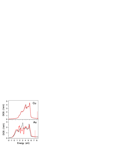
Figure 1: (Color online) Calculated valence band densities of states for Cu and Au bulk without SO interaction (dots) and with SO interaction (solid line). For the latter case the Fermi energies, $\varepsilon_{F}^{Cu}=8.3$ eV and $\varepsilon_{F}^{Au}=7.4$ eV, are indicated by vertical lines.

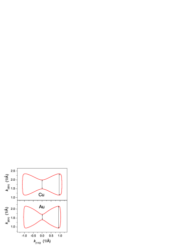
Figure 2: (Color online) Calculated plane cuts perpendicular to the (1 -1 0) direction of the FS of Cu and Au. The arrows denote the extremal vectors of lengths, $Q_{\rm min}^{\rm Cu}=0.505$ Å^-1, $Q_{\rm max}^{\rm Cu}=1.208$ Å^-1 and $Q_{\rm min}^{\rm Au}=0.298$ Å^-1, $Q_{\rm max}^{\rm Au}=1.228$ Å^-1.

As we learned from the asymptotic analysis presented in Sec. II.D, extremal vectors of the Fermi surface play a crucial role in determining the magnetic anisotropy constants. Therefore, we next investigated the plane cuts of the Fermi surface perpendicular to the (1 -1 0) direction. One can easily read off the length of the (001) extremal vectors from the cuts depicted in Fig. 2: The absolute minimum of the width of the Fermi surface, $Q_{\rm min}$, can be found at ${\bf k}=0$, while the maximum width of the corresponding cut, $Q_{\rm max}$, is related to saddle-points of the Fermi surface. In the case of a Cu host the values obtained from our tight-binding analysis, $Q_{\rm min}^{\rm Cu}=0.505$ Å^-1 and $Q_{\rm max}^{\rm Cu}=1.208$ Å^-1 correspond to periods of 12.44 Å and 5.20 Å (6.88 and 2.88 monolayers (ML)) of the oscillations, and agree fairly well with the periods, 6.08 ML and 2.60 ML, calculated by Lathiotakis et al. iec-lath . Similar satisfactory agreement can be found in the case of a Au host between the periods found from our present calculations, 10.34 ML and 2.51 ML, and those calculated by Bruno and Chappert, 8.6 ML and 2.6 ML. iec-bruno It should be noted, however, that the shape of the FS depends very sensitively on the position of the Fermi energy the precise determination of which is a quite subtle task, since for noble metals like Cu and Au the Fermi energy lies in the very flat 4$sp$ band (see also Fig. 1).

IV.2 The magnetic anisotropy constants within the host spin-orbit coupling model

We calculated the spectral function matrices, Eq. (16), at the Fermi energy of Cu and Au using the methods described in Sections II.B. and C., for up to 50 ML below the surface. As a convincing check of our numerical procedure we verified that the structure of the calculated matrices agrees with that derived analytically from symmetry principles. In the case of a Au host, in Fig. 3 we plotted the calculated off-diagonal matrix elements, $\varrho_{5}(\varepsilon_{F})$, $\dots$, $\varrho_{9}(\varepsilon_{F})$, as a function of the distance $d$ from the surface. As expected, large oscillations can be observed for all the spectral functions near the surface ($d<20$ Å). These oscillations, however, survive for large distances only for $\varrho_{6}$, while they are strongly damped in all the other cases. The limiting values of $\varrho_{i}$ correspond to the bulk case and, as we checked, satisfy the conditions, Eq. (20) with less than 1% relative numerical accuracy.

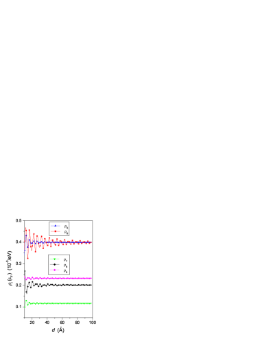
Figure 3: (Color online) Calculated off-diagonal spectral function matrix elements (see Eq. (16)), at the Fermi energy as a function of the distance, $d$, from the (001) surface of a Au host.

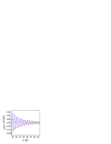
Figure 4: (Color online) Asymptotic fit to the function (31) (solid line) of the calculated values of the $\varrho_{6}(\varepsilon_{F})$ spectral function (triangles) as a function of the distance from a Au(001) surface. The dashed line denotes the bulk value of $\varrho_{6}(\varepsilon_{F})$.

In Fig. 4 we display the spectral function $\varrho_{6}(\varepsilon_{F})$ on an enlarged scale, together with a fitting function of the form, Eq. (31). Quite surprisingly, the asymptotic function applies even in the range of $d\gtrsim 20$ Å and, therefore, there is no need to perform a ’preasymptotic’ analysis as suggested in Ref. orsi4, . The fitted parameters of Eq. (31) are as follows: $\varrho_{6}^{0}(\varepsilon_{F})$ = -3.99 $\pm$ 0.01 $\cdot$ $10^{-4}$ eV^-1, $g_{6}(\varepsilon_{F})$ = -1.484 $\pm$ 0.008 $\cdot$ 10^-3 ÅeV^-1, $Q_{6}(\epsilon_{F})$ = 1.2228 $\pm$ 0.0001 Å^-1, and $\theta_{6}(\epsilon_{F})$ = 1.324 $\pm$ 0.006 rad. It is particularly noteworthy that the fitted wavenumber agrees with an accuracy of 0.5 % with the length of the extremal vector, $Q_{\rm max}$, computed from the Au Fermi Surface. We could fit all other off-diagonal spectral function components entering the expression of $K_{\rm HSO}$ with a similar fit with exactly the same wavenumber. However, the amplitude of these other components was by at least two orders of magnitude smaller than $g_{6}(\varepsilon_{F})$.

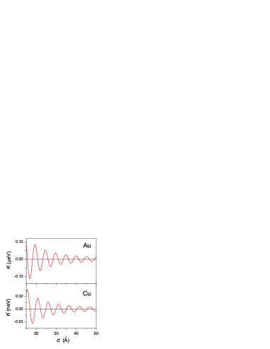
Figure 5: (Color online) Upper panel: The $K^{6}_{HSO}$ contribution to the magnetic anisotropy constant within the host spin-orbit coupling model for a Au host as calculated from the asymptotic expression, Eq. (33). Lower panel: The $K^{9}_{HSO}$ contribution to the magnetic anisotropy constant in the case of a Cu host. In both cases an exchange interaction parameter $J=1$ eV was used.

Our calculations thus indicate that the long-wavelength oscillation corresponding to $Q_{\rm min}$ of the FS either enters with a negligibly small amplitude or doesn’t enter at all in the asymptotic form of the off-diagonal spectral function matrixelements. This can easily be understood by noticing that the asymptotic contributions to the real-space spectral function matrixelements, $\varrho_{s\sigma,s\sigma^{\prime}}^{(q+p)n,(q+p^{\prime})n^{\prime}}(\varepsilon)$ ($p,p^{\prime}=0,\pm 1,d=q\frac{a}{2}$) related to $Q_{\rm min}$ are of the following form,

$$\varrho_{s\sigma,s\sigma^{\prime}}^{(q+p)\,n,(q+p^{\prime})\,n^{\prime}}(\varepsilon) \simeq \varrho_{s\sigma,s\sigma^{\prime}}^{(0)p\,n,p^{\prime}\,n^{\prime}}(\varepsilon)+\frac{g_{s\sigma,s\sigma^{\prime}}^{p,p^{\prime}}(\varepsilon)}{d}\times$$ (36)

$$\cos\left[Q_{\rm min}(\varepsilon)d+\theta(\varepsilon)\right]\;,$$

where $\varrho_{s\sigma,s\sigma^{\prime}}^{(0)p\,n,p^{\prime}\,n^{\prime}}(\varepsilon)$ refer to the corresponding bulk matrixelements. Eq. (36) implies that the oscillating part does not depend on the in-plane positions, $n$ and $n^{\prime}$, which is the consequence that the minimal extremal vector is at the ${\bf k}=0$ point of the 2D Brillouin zone. As explained in Sec. II.B., the matrixelements in Eq. (16) are linear combinations of the above real-space matrix elements according to the states in Table I. Since the states $|\alpha\rangle$ ($\alpha=1,\dots,4$) are constructed as antisymmetric combinations of neighboring $s$-orbitals in the same plane, $q+p$, or as a sum of such antisymmetric combinations, in their matrixelements the asymptotic oscillatory part corresponding to $Q_{\rm min}$ necessarily cancels. As a consequence, only the spectral function $\varrho_{4}\equiv\langle 5|\varrho|5\rangle$ has asymptotic oscillations with wavenumber $Q_{\rm min}$, which, however, does not give a contribution in the host SO model.

We calculated the magnetic anisotropy constant using the asymptotic fits of the spectral functions and Eq. (33). We numerically determined the energy derivative of the magnitude of the extremal vector, $Q^{\prime}(\varepsilon_{F})$, by fitting the spectral functions at two energy values close below and above $\varepsilon_{F}$ and obtained $Q^{\prime}(\epsilon_{F})=0.235$ (Å eV)^-1. Thus, in case of a Au host we get the following asymptotic function for $K^{6}_{HSO}(d)$ (displayed in the upper panel of Fig. 5)

$$K^{6}_{HSO}(d)=\frac{31.66}{d^{2}}\cos\left[1.2228\cdot d+1.324\right]\>\mu{\rm eV}\;,$$ (37)

where $d$ is measured in Å. Notice the surprisingly small magnitude of $K^{6}_{HSO}$: even at a distance of about $d=20$ Å the amplitude of the above oscillating function is about 0.079 $\mu$eV.

We performed similar calculations for a Cu host. In Cu, the spectral functions show asymptotic oscillations with $Q(\varepsilon_{F})=1.205$ Å^-1 that agrees within 0.3 % with the length of the extremal vector, $Q_{\rm max}$, of the Cu FS. In Cu, the $K^{9}_{HSO}$ contribution shown in the lower panel of Fig. 5 dominates the magnetic anisotropy. This is in the range of 0.01 neV = 10^-11 eV, i.e., it is at least by three orders of magnitude smaller than the one found in case a Au host. This decrease is mostly due to the smaller SO interaction in Cu than in Au. As we checked by varying $\xi$ for Au, the spectral functions in Eq. (16) scale linearly with $\xi$, therefore, by Eq. (19) the magnetic anisotropy constant scales as $\sim\xi^{2}$. This result clearly justifies the approach of Újsághy et al., who treated the SO interaction perturbatively.orsi1 ; orsi2 ; orsi3 ; orsi4 .

IV.3 The magnetic anisotropy constants within the local spin-orbit coupling model

As pointed out in Ref. SZG:prl06, , a mechanism based on a strong local SO interaction of the impurity (local SO model) can give rise to a level splitting that is orders of magnitude larger than the host-induced anisotropy. To demonstrate this idea, in Ref. SZG:prl06, we studied the simple but unrealistic case of a single-band metal on a simple cubic lattice. Here we extend the calculations of Ref. SZG:prl06, and perform calculations for realistic host metals (Cu and Au).

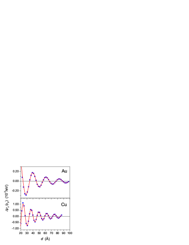
Figure 6: (Color online) Calculated values of $\Delta\varrho_{4}(\varepsilon_{F})\equiv\varrho_{4}(\varepsilon_{F})-\varrho_{4}^{0}(\varepsilon_{F})$ (squares) with corresponding asymptotic fits, Eq. (31), (solid line) as a function of the distance from the (001) surface of Au and Cu.

According to the theory presented in Sec. II.C, we need to compute the diagonal spectral function matrixelements, $\varrho_{3}\equiv\langle 4|\varrho|4\rangle$ and $\varrho_{4}\equiv\langle 5|\varrho|5\rangle$, see Table I and Eq. (16). Our calculations clearly showed that the $d$ dependent Friedel oscillations of $\varrho_{3}$ are several order smaller in magnitude than those of $\varrho_{4}$. This can be understood by noticing that, due to the different spatial character of these two states ($D_{x^{2}-y^{2}}$ and $D_{2z^{2}-x^{2}-y^{2}}$), $\varrho_{3}$ comprises an average of spectral weights in layers $q-1$ and $q+1$, while $\varrho_{4}$ takes the difference of spectral weights in layer $q$ with respect those in layers $q-1$ and $q+1$, $q$ denoting the layer of the impurity’s position. Recalling that for a cubic bulk $\varrho_{3}=\varrho_{4}$, see Eq. (20), in the asymptotic region $K_{\rm LSO}$ becomes proportional with the integral of the function, $\Delta\varrho_{4}(\varepsilon,d)\equiv\varrho_{4}(\varepsilon,d)-\varrho_{4}^{0}(\varepsilon)$. This function is displayed in Fig. 6 for both the Au and the Cu hosts. Remarkably, the amplitude of the Friedel oscillations is about one order of magnitude larger than those of the off-diagonal spectral functions (compare with Fig. 3 for the case of Au). Note that the off-diagonal matrixelements appear in first order of the spin-orbit coupling. The oscillations have larger periods as compared to the off-diagonal spectral functions: a fit to the asymptotic function, Eq. (31), shown also in Fig. 6 gave the values $Q^{Au}=0.292$ Å^-1 and $Q^{Cu}=0.505$ Å^-1, in very good agreement with the length of the small extremal vector, $Q_{\rm min}$, of the corresponding Fermi surfaces. Interestingly, the amplitude of the oscillations is more than three times larger for Cu than for Au: from the fits we obtained $g_{4}(\varepsilon_{F})=1.16\cdot 10^{-2}$ Å eV^-1 and $3.53\cdot 10^{-2}$ Å eV^-1 for the case of Au and Cu, respectively.

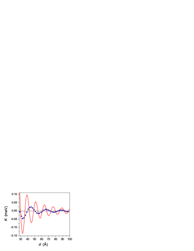
Figure 7: (Color online) Magnetic anisotropy constants within the local spin-orbit coupling model calculated by using the asymptotic formula, Eq. (34), as a function of the distance $d$ from the (001) surface of a Au (dashes) and a Cu host (solid line). In case of Au the squares stand for the magnetic anisotropy constants calculated directly from Eq. (30).

Fig. 7 shows the magnetic anisotropy constants obtained using Eq. (34) with the parameters extracted from the fits of $\Delta\varrho_{4}(\varepsilon_{F},d)$. The parameter $Q^{\prime}(\epsilon_{F})$ was computed as for the off-diagonal spectral functions, and took a value of 0.245 (ÅeV)^-1 for Au and 0.238 (ÅeV)^-1 for Cu. Choosing again $J=1$ eV, we obtained for the amplitudes of the oscillations of $K$, $A(d)=0.0237/d^{2}$ eV and $A(d)=0.0742/d^{2}$ eV ($d$ measured in Å ) in Au and Cu, respectively. In particular, for Cu this gives an amplitude of 0.03 meV at $d=50$ Å or 0.007 meV at $d=100$ Å, which is in the range of $T_{K}$ for typical dilute magnetic alloys, such as Cu(Mn), Cu(Cr).

In Fig. 7, we also compare the magnetic anisotropy constants obtained from the asymptotic analysis with the values we get by performing the contour integration in Eq. (30). Apparently, already for $d>35$ Å, these values lie almost perfectly on the asymptotic curve. This nice agreement proves the validity of the asymptotic formula, Eq. (34), as well as the accuracy of our numerical procedure to compute the magnetic anisotropy constant.

V Summary and conclusions

In this paper, we performed a theoretical study of two mechanisms for surface-induced magnetic anisotropy of a magnetic impurity: a local spin-orbit mechanism (LSO),SZG:prl06 and a host spin-orbit mechanism (HSO).orsi1 Both mechanisms appear as a result of Friedel-like oscillations in the local spectral functions, induced by the surface. In the local SO mechanism, the rather large diagonal, i.e., charge oscillations couple through the local spin-orbit coupling on the d- or f-level of the magnetic impurity to the impurity spin and lead to a surface-induced splitting of the spin states. The host SO mechanism, on the other hand, relies on oscillations in the off-diagonal elements of the local spectral functions, i.e., oscillations in the “spin sector” that couple directly to the spin through an exchange interaction. These oscillations are induced by the SO coupling in the host metal and, thus, they are much weaker than the Friedel oscillations in the ”charge sector”. Based upon this simple picture, one therefore expects that the first mechanism is dominant for impurities with a partially filled d- or f-shell, while the host SO mechanism may become important for half-filled shells, in which case the local SO mechanism cannot be at work.

In this paper we attempted to compare these two mechanisms quantitatively. For the description of the host’s valence and conduction electrons we used a tight-binding Green’s function technique, which allows for a perfect treatment of the semi-infinite surface geometry, and makes also possible a non-perturbative treatment of the host SO interaction. We then used a field theoretical approach to compute the self-energy of the spin up to first (local SO) and second orders in the exchange coupling, $J$, (host SO model), and derived explicit expressions for the anisotropy constants, $K$, as a function of the separation $d$ between the impurity and the surface.

These expressions have been analyzed using an asymptotic analysis which resulted in a very similar oscillatory dependence of $K$ on $d$ in both models: the periods of the oscillations could be identified as the magnitudes of the extremal vectors of the Fermi Surface of the bulk host and their amplitudes decayed in both models as 1/$d^{2}$. Here we must remark that in our calculations in Ref. SZG:prl06, we predicted a $1/d^{3}$ decay of the oscillations of $K$ within the host spin-orbit mechanism. This must be contrasted to the results of the present work, where we find rather a $1/d^{2}$ scaling of the host-induced anisotropy. This apparent controversy is due to a small difference in the calculations: Unlike the present work, in Ref. SZG:prl06, we neglected the potential scattering at the impurity site, i.e., we used the local spectral functions of a perfect semi-infinite host. In this case, however, one can show that certain off-diagonal elements of the local spectral function matrix must vanish due to two-dimensional translational symmetry. These off-diagonal matrix elements are non-zero, once translational invariance is broken by potential scattering at the impurity site, and they give rise to a $1/d^{2}$ decay of the anisotropy as shown in Sec. II.D.

Using realistic tight-binding parameters, we calculated the amplitudes of the magnetic anisotropy oscillations for the cases of Au and Cu metal hosts. As expected from the very different SO interactions in these metals, within the host SO model, the magnetic anisotropy constant for Au turned out to be about three orders larger in magnitude than for Cu. Nevertheless, even for a Au host and close to the surface, the magnetic anisotropy constants remained below the range of 0.1 $\mu$eV. Though a direct comparison with the result of Ref. orsi4, is quite questionable mainly due to the different geometrical distribution of the host atoms and to the different approximations used, the above value is close to the lower limit of the estimated range of $K$ given in Ref. orsi4, . We therefore conclude that most probably the host SO mechanism of Ref. orsi4, is too weak to explain the size-dependence of the Kondo resistance.

The local SO mechanism proposed in Ref. SZG:prl06, , on the other hand, gives a magnetic anisotropy constants for Cu in the range of 0.03-0.01 meV for even at distances 50-100 Å away from the surface. Although they are in the same range, the magnetic anisotropy constants for Au were about three times smaller than the ones we got for Cu. Our numerical studies imply that the primary mechanism to produce a magnetic anisotropy in the vicinity of a surface is provided by the local SO coupling, where the local Hund’s rule coupling conspires with Friedel oscillations to produce a large anisotropy effect. This mechanism seems to be large enough to explain the suppression of the Kondo resistance anomaly observed in thin films and it also supposed to be the dominant source of (random) magnetic anisotropy in metallic mesoscopic structures such as metallic nano-grains, nano-wires, or point contacts.

The authors are indebted to A. Zawadowski and O. Újsághy for valuable discussions. This work has been financed by the Hungarian National Scientific Research Foundation (OTKA T068312 and NF061726) and by a cooperation between the Spanish Ministry of Science and the Hungarian Science and Technology Foundation (HH2006-0027 and OMFB-01230/2007).

References

- (1) Guanlong Chen and N. Giordano, Phys. Rev. Lett. 66, 209 (1991).
- (2) J.F. DiTusa, K. Lin, M. Park, M.S. Isaacson, and J.M. Parpia, Phys. Rev. Lett. 68, 1156 (1992).
- (3) M.A. Blachly and N. Giordano, Europhys. Lett. 27, 687 (1994); Phys. Rev. B 49, 6788 (1994); Physica (Amsterdam) 194B–196B, 983 (1994).
- (4) N. Giordano, Phys. Rev. B. 53, 2487 (1996).
- (5) O. Újsághy, A. Zawadowski, and B.L. Györffy, Phys. Rev. Lett. 76, 2378 (1996).
- (6) O. Újsághy and A. Zawadowski, Phys. Rev. B 57, 11598 (1998)
- (7) O. Újsághy, L. Borda, and A. Zawadowski, J. Appl. Phys. 87, 6083 (2000).
- (8) T. M. Jacobs and N. Giordano, Europhys. Lett. 44 74-79 (1998); Phys. Rev. B 62, 14145 (2000).
- (9) O. Újsághy, L. Szunyogh, and A. Zawadowski, Phys. Rev. B 75, 064425 (2007).
- (10) We note that Eq. (2) refers to a homogeneous distribution of host atoms (spin-orbit scatterers), while for the case of a layered geometry and phase coherence, , and being the interlayer distance and an integer, respectively, a slower decay, , has been predicted.orsi4
- (11) L. Szunyogh and B. L. Györffy, Phys. Rev. Lett. 78, 3765 (1997).
- (12) L. Szunyogh, G. Zaránd, S. Gallego, M. C. Muñoz, and B. L. Györffy, Phys. Rev. Lett. 96, 067204 (2006).
- (13) M. C. Muñoz, V. R. Velasco, and F. Garcia–Moliner, Phys. Scr. 35, 504 (1987); M. C. Muñoz and M. P. López Sancho, Phys. Rev. B 41, 8412 (1990).
- (14) D.L. Cox and A. Zawadowski, Adv. Phys. 47, 599 (1998).
- (15) A. A. Abrikosov, Physics (Long Island City, NY) 2, 5 (1965).
- (16) J. R. Schrieffer and P. A. Wolff, Phys. Rev. 149, 491 (1966).
- (17) B. Coqblin and J. R. Schrieffer, Phys. Rev. 185, 847 (1969).
- (18) N.D. Lang and W. Kohn, Phys. Rev. B 1, 4555 (1970); ibid. 3, 1215 (1971); ibid. 7, 3541 (1973).
- (19) A. Papaconstantopoulos, Handbook of Electronic Structure of Elemental Solids, Plenum, New York, 1986, p. 199.
- (20) S. Gallego, F. Soria, and M.C.Muñoz, Surface Science 524, 164-172 (2003).
- (21) http://www.webelements.com/
- (22) L. Szunyogh, B. Újfalussy, P. Weinberger, and J. Kollár, J. Phys.: Condensed Matter. 6, 3301-3306 (1994).
- (23) L. Szunyogh, B. Újfalussy, P. Weinberger, and J. Kollár, Phys. Rev. B 49, 2721 (1994).
- (24) N.N. Lathiotakis, B.L. Györffy, J.B. Staunton, and B. Újfalussy, Journal of Magnetism and Magnetic Materials 185, 293-304 (1998).
- (25) P. Bruno and C. Chappert, Phys. Rev. Lett. 67, 1602 (1991); 67 2592(E) (1991).