Compressing Binary Decision Diagrams

Abstract

The paper introduces a new technique for compressing Binary Decision Diagrams in those cases where random access is not required. Using this technique, compression and decompression can be done in linear time in the size of the BDD and compression will in many cases reduce the size of the BDD to 1-2 bits per node.

Empirical results for our compression technique are presented, including comparisons with previously introduced techniques, showing that the new technique dominate on all tested instances.

1 Introduction

In this paper we introduce a technique for compressing binary decision diagrams for those cases where random access to the compressed representation is not needed. We will use the term offline to describe a BDD stored in such a manner that it no longer allows random access to its structure without decompressing the BDD first. The two primary areas in which decision diagrams are used in practice are verification and configuration. In both of these areas it is sometimes important to store binary decision diagrams offline using as little space as possible. Primarily the need for such compression arises when it is necessary to transmit binary decision diagrams across communication channels with limited bandwidth. In the area of verification this need arises for example when using a networked cluster of computers to perform a distributed compilation of a binary decision diagram [1]. A similar exchange of BDD data takes place in distributed configuration as described in [13]. In such approaches the fact that the network bandwidth is much lower than the memory bandwidth can become a major bottleneck as computers stall waiting to receive data to process. Transmitting the binary decision diagrams in a compressed representation can help alleviate this problem. The same problem arises in standard interactive configuration. Consider for example a web-based interactive configurator that uses BDDs to store the set of valid configurations. It must either transmit the BDD storing the configuration data to the customers computer or perform all computations on the server leading to a network delay each time the user makes a choice during the configuration. In order to reduce the required bandwidth as well as lower the load time in the first case, it is benefical to transmit the BDD in a compressed format.

The paper is organized as follows: In Section 2 we present the neccessary notation and definitions. In Section 3 we present our compression scheme. Finally, in Section 4 we show the compression attained by applying our compression scheme on different instances.

1.1 Related work

Most of the work done on compressing decision diagrams aim to achieve large reductions in size, while maintaining random access, by means of better variable orderings [7][3] or modifications to the decision diagram data structure [4]. Such work is mostly orthogonal to the aim of this paper, as the compression strategy we present easily can be adapted for use with the variations over basic BDDs.

The only previous work we are aware of for compressing BDDs for offline storage is the work by Starkey and Bryant[11] and the follow-up paper by Mateu and Prades-Nebot[8] which both describes techniques for image compression using BDDs. The latter of these includes a non-trivial encoding algorithm for storing the BDD offline. Finally Kieffer et.al[5] gives theoretical results for using BDDs for general data compression including a technique for storing BDDs. After presenting our own technique, we present empirical results comparing the new encoder with the encoders from [8] and [5].

2 Preliminaries

Definition 1 (Ordered Binary Decision Diagram).

[2] An ordered binary decision diagram on $n$ binary variables $X=\{x_{1},\ldots,x_{n}\}$ is a layered directed acyclic graph $G(V,E)$ with $n+1$ layers (some of which may be empty) and exactly one root. We use $l(u)$ to denote the layer in which the node $u$ resides. In addition the following properties must be satisfied:

• If $|V|\neq 1$, there are exactly two nodes in layer $n+1$. These nodes have no outgoing edges and are denoted the 1-terminal and the 0-terminal. If $|V|=1$ the layer will either contain the 1-terminal or the 0-terminal.

• All nodes in layer $1$ to $n$ have exactly two outgoing edges, denoted the low and high edge respectively. We use $low(u)$ and $high(u)$ to denote the end-point of the low and high edge of $u$ respectively.

• For any edge $(u,v)\in E$ it is the case that $l(u)<l(v)$

We use $E_{low}$ and $E_{high}$ to denote the set of low and high edges respectively. An edge $(u,v)$ such that $l(u)+1<l(v)$ is called a long edge and is said to skip layer $l(u)+1$ to $l(v)-1$. The length of an edge $(u,v)$ is defined as $l(v)-l(u)$.

Definition 2 (Reduced ordered Binary Decision Diagram).

An ordered Binary Decision Diagram is called reduced iff for any two distinct nodes $u,v$ it holds that $low(u)\not=low(v)\lor high(u)\not=high(v)$ and further that $high(u)\not=low(u)$ for all nodes $u$.

In the rest of this paper we will assume for all BDDs we are considering that they are ordered and reduced.

Definition 3 (Solution to a BDD).

A complete assignment $\rho$ to $X$ is a solution to an BDD $G(V,E)$ iff there exists a path $P$ from the root in $G$ to the 1-terminal such that for every assignment $(x_{i},b)\in\rho$, where $b\in\{low,high\}$, there exists an edge $(u,v)$ in $P$ such that one of the following holds:

• $l(u)<i<l(v)$

• $l(u)=i$ and $(u,v)\in E_{b}$

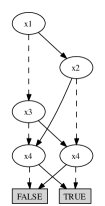
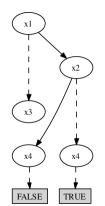
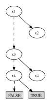
Figure 1: From left to right: A BDD and two different spanning trees on the BDD. Solid and dashed edges corresponds to high and low edges respectively

Example 4.

Figure 1 contains a BDD on the binary variables $X=\{x_{1},x_{2},x_{3},x_{4}\}$ which the solutions $\{(1,1,1,1),$ $(1,1,0,1),$ $(1,0,1,0),$ $(1,0,0,0),$ $(0,1,1,0),$ $(0,1,0,1),$ $(0,0,1,0),$ $(0,0,0,1)\}$.

Definition 5 (BFS order).

A BFS ordering $id_{b}:V\rightarrow\{1,\ldots,|V|\}$ of the nodes in a layered DAG $G(V,E)$ rooted in $r$ is the ordering of $V$ in the order they are visited by a BFS in the DAG starting at $r$ and traversing left edges prior to right edges.

Definition 6 (Layer order).

A layer ordering $id_{l}:V\rightarrow\{1,\ldots,|V|\}$ of the nodes in a layered DAG $G(V,E)$ rooted in $r$ is the ordering of $V$ layer by layer in increasing order of the layer. Nodes at the same layer are ordered in the order that they are visited by a DFS in the DAG starting at $r$ and traversing left edges prior to right edges.

We refer to $id_{b}(v)$ and $id_{l}(v)$ by “the BFS id of $v$” and “the layer id of $v$” respectively. Note that if all edges in a layered DAG has the same length then the ordering $id_{l}$ and $id_{b}$ will be the same.

In our compression scheme we will make use of the following well-known fact:

Lemma 7.

Every binary tree can be unambiguously encoded using 2 bits pr. node.

To achieve such an encoding each node $v$ is encoded using two bits. The first bit and the second bit is true iff $v$ contains a left and a right child respectively. In order to make decoding possible the order in which the children of already decoded nodes appear in the encoded data must be known. This can for example be ensured by encoding the nodes in a DFS or BFS order with either left-first or right-first traversal. As an example, the encoding of the nodes of the binary tree in Figure 1 in BFS order is $(11,11,00,11,00,00,00)$.

3 The Compression technique

Our compression technique can be summarized by the following steps:

1. Build a spanning tree on the BDD (Section 3.1).

2. Encode edges in the spanning tree, using Lemma 7

3. Encode by one bit the order in which the two terminals appear in the spanning tree.

4. Encode the length of the edges in the spanning tree where necessary (Section 3.2).

5. Encode the edges that are not in the spanning tree (Section 3.3).

6. Compress the resulting data using standard compression techniques.

The decoder starts by reverting step (6) by decompressing the data. It then recreates the binary tree (1-2), restores the correct layer of each node (4), and restores the remaining missing edges (5). Below we give the details of each step.

3.1 Building the spanning tree on the BDD

Definition 8 (Spanning Tree).

A spanning tree $G^{T}(V^{T},E^{T})$ on a BDD $G(V,E)$ is a subgraph of $G$, for which $V^{T}=V$, and any two vertices are connected by exactly one path of edges in $E^{T}$. An edge is called a tree edge if it is contained in the spanning tree and a nontree edge otherwise.

The most obvious way to construct a spanning tree on a graph is to use DFS or BFS. In the case of a rooted DAG one can obtain a spanning tree by, for each node $v$ except the root, adding a single edge with endpoint in $v$ to the set of tree edges. Two examples of spanning trees for the BDD in Figure 1 are shown in Figure 1 and 1.

In our encoder we will construct a spanning tree containing as few long edges as possible. Hence when a node $v$ in the BDD has multiple parents $u_{1},\ldots,u_{k}$ and we have to choose one of the edges $(u_{1},v),\ldots,(u_{k},v)$ to add to the spanning tree, we will always choose the shortest possible edge, that is an edge $(u_{i},v)$ where $l(u_{i})\geq l(u_{1}),\ldots,l(u_{k})$. Ties are broken by choosing the edge $(u,v)$ with the smallest $id_{l}(u)$. Note that the resulting spanning tree is uniquely defined regardless of which order we process nodes in. Using this construction we achieve a spanning tree with a minimal number of long edges. This can easily be seen by noting that precisely one ingoing edge must be chosen for each node, and additionally that the choice of one edge can never exclude an edge to another node from consideration.

Example 9.

The spanning tree in Figure 1 contains three long edges, whereas the spanning tree in Figure 1 only contains one. The latter of these would be the one constructed by our encoder upon compressing the BDD in Figure 1. The single long edge in figure 1 has to be included in the tree as it is the only possible way for the spanning tree to include the node in layer 1.

3.2 Encoding the lengths of the tree edges

The spanning tree is stored as a binary tree where all edges have the same length. Since some of the edges in the spanning tree may correspond to long edges in the BDD, the binary tree itself may not be sufficient to reconstruct the layer information of the nodes during decoding. In order to enable the decoder to deduce the correct layer we therefore encode the location and the length of each long edge that is included in the spanning tree. The location of a long edge $(u,v)$ is uniquely specified by the BFS order of the end point of the edge, that is $id_{b}(v)$.

When encoding the location of the long edges $(u_{1},v_{1}),\ldots,(u_{k},v_{k})$ we will, instead of outputting the integers $id_{b}(v_{1}),\ldots id_{b}(v_{k})$, output a bitvector of length $|V|$ for which entries $id_{b}(v_{1}),\ldots,id_{b}(v_{k})$ are true and all other entries are false. Though this encoding is likely to require more bits than encoding by listing the integers, the bitvector will be compressed very efficiently when the standard compression is applied in the final phase.

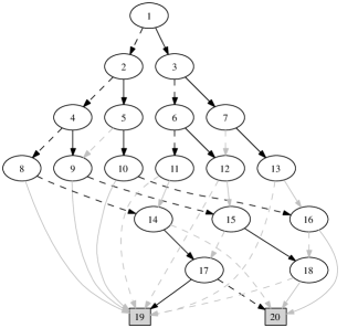
Figure 2: A spanning tree on a BDD. The black edges are tree edges and the gray edges are nontree edges. The nodes are labeled in layer order

3.3 Encoding nontree edges

When the spanning tree and the layer information is encoded, we only need to encode the nontree edges, that is, those edges in the BDD that are not contained in the spanning tree.

We know that half of the edges in the BDD will be encoded as nontree edges as it follows from the following observation:

Observation 10.

Let $G(V,E)$ be a BDD containing at least $3$ nodes. Then any spanning tree on $G$ will contain exactly $|E|/2+1$ edges

Proof.

By the assumption that $|V|>2$, it holds for any BDD $G(V,E)$ that $|E|=2(|V|-2)$, since all nodes in a BDD except the two terminals have two children. Further any tree with $|V|$ nodes contains $|V|-1$ edges, which equals $|E|/2+1$ edges. ∎

As an example the construction in Figure 2 contains 19 tree edges and 17 nontree edges.

Since every node except the terminals in the BDD has two children and we have the spanning tree available with restored layer information, we know the start point of each of the nontree edges that has to be added to the spanning tree in order to reconstruct the BDD. Hence if we encode the nontree edges in some fixed order according to their start point then we only need to encode the end point of each of the nontree edges. We will call the endpoint of any nontree edge that has yet to be encoded an incomplete child. By $S$, we will denote the sequence of incomplete children in the order in which their parents appear in the layer ordering of the nodes, that is $S=(v_{1},\ldots,v_{k})$ for the nontree edges $(u_{1},v_{1}),\ldots,(u_{k},v_{k})$. By $id_{l}(S)$ we denote the corresponding sequence of layer ids, that is $id_{l}(S)=(id_{l}(v_{1}),\ldots,id_{l}(v_{k}))$.

We will now describe three encodings of nontree edges in Section 3.3.1, Section 3.3.2 and Section 3.3.3 which we will combine to encode all the nontree edges.

3.3.1 Incomplete children with large in-degree

In order for a standard compression technique to successfully compress the sequence $id_{l}(S)$ it is important that the symbols in the sequence appears with high frequency. We note that nodes with in-degree $d$ will appear $d-1$ times in the sequence of nontree edges. Hence by applying standard compression we will be able to efficiently compress those nontree children that have a high in-degree if they are separated from the nodes that have a low in-degree. Therefore we split the sequence of nodes appearing as incomplete children in $S$ into two disjoint subsequences $H$ and $L$, the first containing those incomplete children that have an in-degree larger than a specified threshold in their order of appearence in $S$, the latter containing the rest. For example if the threshold is 3 then $H=(19,19,19,19,19,19,19,19,20,20,20,20)$ for the BDD in Figure 2. Based on $H$ we construct the sequence of integers $S^{H}$ on the sequence of nodes $v_{1},\ldots,v_{|V|}$ in $S$ by encoding $v_{i}\in H$ as $id_{l}(v_{i})$ and $v_{i}\in L$ as $0$. By the encoded $0$s we indicate the incomplete children that are not among the incomplete children with high in-degree. Note that all integers appearing in $S^{H}$ occurs with a high frequency and therefore will compress efficiently using standard compression techniques. The remaining incomplete children $L$, we code separately, as described in the next two sections.

3.3.2 Incomplete children with small in-degree

Using the above encoding, we are left with a sequence of nontree children $L$, with very few repetitions. When encoding this sequence we will exploit the fact that the sequence of integers in $id_{l}(L)$ will in most instances tend to be increasing. Below we argue why this is the case.

1. The first reason is that any node $u$, with an outgoing edge of length $k$ is naturally restricted to the children occurring in layer $l(u)+k$, and therefore to the range of $id_{l}$ indices of the nodes at layer $l(u)+k$. Since most edges in a BDD are usually rather short (except those to the terminals), this leads to a natural increasing progression in $id_{l}(L)$.

2. Secondly, when examining a set of layers in a BDD it is very common to see disjoint substructures. For example, in Figure 2, we have two disjoint substructures induced by the nodes $2,4,5,8,9,10$ and $3,6,7,11,12,13$. Given two disjoint substructures then for any given layer $l$ let $I^{l}_{1}$ and $I^{l}_{2}$ be the sequences of layer indices of the nodes in that layer from each of them respectively. Assume for convinience that $I^{l}_{1}$ contains the smallest index. Then it is the case that all indices in $I^{l}_{1}$ are strictly smaller than all indices in $I^{l}_{2}$, and furthermore the same applies to $I^{j}_{1}$ and $I^{j}_{2}$ for any other layer $j$. Since the incomplete children of a layer are encoded according to the order of their parents, this means that $I^{i}_{1}$ will always appear in $id_{l}(L)$ before $I^{i}_{2}$ for any layer $i$, helping to ensure an increasing tendency in $id_{l}(L)$.

3. Thirdly, some possible nontree edges cannot exist, since had they in fact existed they would have been included in the spanning tree. This constraint on the nontree edges is stated in the following observation:

   Observation 11.

   For every nontree edge $(u,v)$ it holds that

   $$v\not\in\{v^{\prime}\mid\exists(u^{\prime},v^{\prime})\in E^{T}:l(u^{\prime})=l(u)\land id_{l}(u)<id_{l}(u^{\prime})\}$$

   In other words: assume that there is a nontree edge $(u,v)$ for which a right sibling $u^{\prime}$ of $u$ has the child $v^{\prime}$ in the spanning tree, then $v\neq v^{\prime}$.

   Proof.

   If $v=v^{\prime}$ then since $u$ and $u^{\prime}$ are on the same layer, and since $id_{l}(u)<id_{l}(u^{\prime})$ the spanning tree would contain $(u,v)$ rather than $(u^{\prime},v)$, which contradicts that $(u,v)$ is a nontree edge. This is due to the fact that when the spanning tree is constructed by a traversal of the nodes in the BDD in layer order. ∎

   Example 12.

   In Figure 2 an incomplete child of the node $5$ can neither be $11,12$ or $13$, since in that case the corresponding edge would be a tree edge, which contradict that the child is incomplete. On the other hand an incomplete child of $7$ can be any of the nodes $8,\ldots,12$ since $7$ is positioned to the right of all its siblings.

   What follows from Observation 11 is, roughly stated, that incomplete children with parents in the “left part” of a layer are bound to have one of the smaller layer ids in the layer, whereas the incomplete children with parents in the “right part” of the of a layer can have any layer id occurring in the layer.

As a conclusion of three the reasons mentioned above about why we expect the sequence of incomplete children to tend towards being increasing, and as we have observed the increasing trend of $id(L)$ in the instances we have tested on, we choose to exploit this fact by encoding the sequence $id_{l}(L)$ by delta coding:

Definition 13 (Delta Coding).

Consider any sequence of integers $(i_{1},\ldots i_{k})\in\mathbb{Z}^{k}$ for any $k\in\mathbb{N}$. We define the delta coding of $(i_{1},\ldots i_{k})$ by $\Delta(i_{1},\ldots i_{k})=(i_{1},i_{2}-i_{1},i_{3}-i_{2},\ldots,i_{k}-i_{k-1})$

For instance if $id_{l}(L)=(9,12,14,15,16,17,18,20)$, then $\Delta(id_{l}(L))=(9,3,2,1,1,1,1,2)$. Standard compression will be able to compress the latter sequence much better than the former sequence.

3.3.3 Long forward edges

Using the encoding of Section 3.3.2 nontree long edges will often be expensive to encode since they have an incomplete child with an id that is a lot larger than for the short edges. Hence they will often result in large deltas in the delta coding. The following approach is an alternative way of encoding some of the long edges. This technique is therefore applied prior to the technique in Section 3.3.2 and only the remaining edges will be coded using delta-coding.

A nontree edge $(u,v)$ is a forward edge if $u$ is an ancestor of $v$ in the spanning tree. Consider any forward edge $(u,v)$ in the graph with length $k$. This edge can be unambiguously encoded by $id_{l}(v)$ and the length of the edge, as $u$ if the ancestor of $v$ at layer $l(v)-k$.

In order to know which nodes that are endpoints of forward edges we label each node $v$ by the number of forward edges ending in $v$. This will be $0$ for most nodes and very seldom be more than $1$, ensuring a good compression of the labelling. After this is done we encode the length of the forward edges. If there are very few long edges it might not be worth the effort to write the labelling on the edges. Hence we set a threshold on the number of forward edges that it needed in order to make the encoding of these edges useful. If the threshold is not exceeded all long forward edges are instead encoded as described in Section 3.3.2.

3.4 An example

As a final part in the description of our compression technique, we show how our technique would compress the BDD in Figure 2.

Example 14.

Consider the encoding of the BDD in Figure 2. We first use Lemma 7 to encode the spanning tree as the bitstring (comma separated only to ease readability) $11,1111,11011101,101010000000,010100,1100,0000$. As there are no long edges in the spanning tree we do not need to encode layer information, we will output $0$ to denote that the total number of layer information that is to be added is $0$. If we suppose a threshold of $5$ in the encoding of nontree edges with high indegree only the node $19$ will be encoded as an incomplete child with high indegree. This will be encoded as $0\;0\;19\;19\;19\;19\;0\;19\;0\;19\;0\;0\;0\;0\;0\;19\;0$

We are now left with two long forward edges of length 2, namely $(14,20)$ and $(16,20)$. To encode them we first specify which of the remaining nontree edges that are long forward edges by a bitvector $0000010010$ and the length $2,2$. Finally we encode the remain nontree edges by $9\;12\;14\;15\;16\;17\;18\;20$ which in delta coding will be $9\;3\;2\;1\;1\;1\;1\;2$.

4 Experiments

In this section we provide empirical results from compressing a large set of BDDs from various sources using the new encoder described in this paper and as well as the encoders from [8] and [5]. For further comparison we also provide the results from a naive encoder. The naive encoder outputs the size of each layer followed by a list of children. This representation is very similar to the in-memory representation of a BDD except that the layer information is not stored for each node but rather implicitly using the layer sizes.

4.1 Instances

Many of the instances we show results for are taken from the configuration library CLib [12]. As a BDD only allows binary variables, additional steps must be taken in order to encode solutions to problems containing variables with domains of size larger than 2. For each non-binary variable in a problem its customary to either use a number of binary variables logarithmic in the size of the domain of the variable and adjust the constraints accordingly or use one variable for each domain value. These methods are known as log-encoding[14] and direct-encoding respectively. In the instances we have tested with all those named with the suffix “dir” was compiled using direct encoding, while the remaining were build using log-encoding. The instances fall into the following groups:

Product Configuration

The instances in this group are all BDDs compiled for use with standard interactive product configurators. For example the “renault” instance is a car configuration instance, and the others are various PC configuration instances.

Power Supply Restoration

These instances were compiled for use in configuring the restoration of a power supply grid after a failure. As such they are also a type of configuration instances.

Fault Trees

These are instances built for use in reliability analysis using fault trees.

Combinatorial

The combinatorial group contains various “toy” chess problems of a combinatorial nature. For example the classic problem of placing 8 queens on a chessboard without any piece being threatened is represented by the instance “8x8queen”. The “5x27queens” instance models placing 5 queens on a 5x27 chess board.

Multipliers

This group contains two BDDs both of which represent the value of the middle bit in the output obtained by multiplying two groups of 10 input bits [9]. These are build mixing the input bits (“mult-mix-10”) and separating the input bits (“mult-apart-10”).

4.2 Post compression

All the tested encoders create an encoding that is meant to be subsequently compressed using standard entropy coding methods. In [8] arithmetic coding is used while the choice of entropy coding is not discussed in [5]. To avoid the empirical results being affected by the choice of standard coding, we instead apply LZMA[10] to the output of all encoders to produce the final encoding. Due to implementation details of this final compression step, it is sometimes beneficial to produce the output that has to be compressed on a byte level instead of a bit level. To ensure a fair comparison the results stated for [8], [5] and the naive approach are obtained by trying to output both on bit level and on byte level and stating the best compression among the two results. Our own encoder was only tested outputting on a byte level.

4.3 Conclusions

From the empirical results shown in Figure 3 we can immediately see that it is worthwhile to make use of a dedicated BDD encoder, as the naive encoding, being only compressed by LZMA, is outperformed with a factor of up to 20 on some instances. Furthermore we can see that the encoder introduced in this paper is consistently able to perform as well or better than the other encoders on all tested instances. In particular the largest BDD in our test (“complex-P3”) required about twice as much space when using either of the two other dedicated encoders.

Instance properties

For most of the instances included here it is the case that a very large fraction (30% to nearly 50%) of the edges lead to the zero-terminal. The exception to this are the multiplier instances, “5x27queens” and the “rook” instances. Slightly less expected is the fact that it is quite rare for nodes other than the zero-terminal to have a significant in-degree, this only occurring with any great significance in “5x27queens” and to lesser extent in “complex-P2” and the multipliers. This means that in quite a few cases nearly all of the non-tree edges are simply edges to the zero-terminal, essentially turning $S^{H}$ into a bitvector, marking almost all the edges as zero-terminal edges, allowing for very efficient compression. This can be seen in the results where the “5x27queens”, the rook and the multiplier instances all turn out to compress less efficiently. An additional important trend is that nodes which cannot be reached by following a short edge from a parent are very rare, meaning that our encoder in by far the most cases only need to provide layer information for less than $1\%$ of the nodes, which is a significant advantage over previous encoders.

Availability

The Java source code used for these experiments (including a command-line encoder and decoder for BDDs in the BuDDy [6] file format) is available along with all instances used in these experiments at (URL removed for blind review).

Name	$|V|$	this paper	[8]	[5]	Naive
Product Configuration
renault	455798	0,90	126%	103%	402 %
renault-dir	1392863	0,23	198%	214%	1352%
pc-CP	16496	0,76	220%	209%	788 %
pc	3467	2,19	224%	211%	436 %
Big-PC	356696	0,38	334%	266%	1345%
Big-PC-dir	1291600	0,17	260%	260%	2035%
Power Supply Restoration
complex-P3	2812872	0,44	243%	202%	951 %
complex-P2	163432	1,16	181%	167%	541 %
1-6+22-32	20937	1,89	136%	154%	413 %
1-6+22-32-dir	61944	0,99	135%	161%	606 %
Fault Trees
isp9607	228706	0,63	389%	204%	873 %
isp9605	4570	3,30	130%	145%	305 %
chinese	3590	2,06	214%	160%	450 %
Combinatorial
5x27queens	562764	4,33	108%	109%	204 %
13x13rook	76808	3,56	210%	165%	311 %
8x8rook	1339	6,03	140%	139%	277 %
8x8queen-dir	2453	2,17	115%	178%	374 %
8x8queen	879	4,29	114%	138%	332 %
Multipliers
mult-mix-10	42468	9,92*	114%	107%	169 %
mult-apart-10	31260	8,07*	120%	124%	202 %

Figure 3: The above table shows the name and size (in nodes) of each of the instances tested. The result of the new encoder, in bits per node, is then showed, followed by the relative results of the rest of the encoders. The * indicates results obtained from our encoder when delta coding is not used in the encoding of nontree edges.

References

- [1] P. Arunachalam, C. Chase, and D. Moundanos, ‘Distributed binary decision diagrams for verification of large circuits’, ICCD, 00, 365, (1996).
- [2] Randal E. Bryant, ‘Graph-based algorithms for boolean function manipulation’, IEEE Transactions on Computers, 35(8), 677–691, (1986).
- [3] S. J. Friedman and K. J. Supowit, ‘Finding the optimal variable ordering for binary decision diagrams’, IEEE Trans. Comput., 39(5), 710–713, (1990).
- [4] Esben Rune Hansen and Peter Tiedemann, ‘Compressing configuration data for memory limited devices’, in AAAI-07, p. 15, (2007).
- [5] J. Kieffer, P. Flajolet, and E h. Yang, ‘Universal lossless data compression via binary decision diagrams’, in Proceedings of ISIT 2000, (2000).
-
[6]
J. Lind-Nielsen, ‘BuDDy - A Binary Decision Diagram Package’.
http://sourceforge.net/projects/buddy, online. - [7] S. Malik, A.R. Wang, R.K. Brayton, and A. Sangiovanni-Vincentelli, ‘Logic verification using binary decision diagrams in a logicsynthesis environment’, in Proc. IEEE International Conference on Computer-Aided Design, pp. 6–9, (1988).
- [8] P. Mateu-Villarroya and J. Prades-Nebot, ‘Lossless image compression using ordered binary-decision diagrams’, Electronic Letters, 37, 162–163, (2001).
- [9] Christoph Meinel and Thorsten Theobald, Algorithms and Data Structures in VLSI Design, Springer-Verlag New York, Inc., Secaucus, NJ, USA, 1998.
- [10] Igor Pavlov. 7z lzma sdk. http://www.7-zip.org/sdk.html.
- [11] M. Starkey and R. Bryant. Using ordered binary-decision diagrams for compressing images and image sequences, 1995.
- [12] Sathiamoorthy Subbarayan. Clib: configuration benchmarks library. http://www.itu.dk/research/cla/externals/clib.
- [13] Peter Tiedemann, Tarik Hadzic, Stuart Henney, and Henrik Reif Andersen, ‘Interactive distributed configuration’, in Proceedings of CP2006, pp. 761–765. Springer-Verlag Berlin Heidelberg, (2006).
- [14] Ingo Wegener, Branching Programs and Binary Decision Diagrams, SIAM Monographs on Discrete Mathematics and Applications, 2000.