Density engineering of an oscillating soliton/vortex ring in a Bose-Einstein condensate

Abstract

When two Bose-Einstein condensates (BEC’s) collide with high collisional energy, the celebrated matter wave interference pattern results. For lower collisional energies the repulsive interaction energy becomes significant, and the interference pattern evolves into an array of grey solitons. The lowest collisional energy, producing a single pair of solitons, has not been probed. We use density engineering on the healing length scale to produce such a pair of solitons. These solitons then evolve periodically between vortex rings and solitons, which we image in-situ on the healing length scale. The stable, periodic evolution is in sharp contrast to the behavior of previous experiments, in which the solitons decay irreversibly into vortex rings via the snake instability. The evolution can be understood in terms of conservation of mass and energy in a narrow condensate. The periodic oscillation between two qualitatively different forms seems to be a rare phenomenon in nature.

We consider two condensates separated in space, and given an initial collisional energy $E_{\text{col}}$, which could be in the form of kinetic energy, or potential energy in a magnetic trap. The condensates are then allowed to collide in the $z$ direction. For negligible interactions, the two colliding condensates will interfere like two non-interacting plane waves, forming a standing wave interference pattern with wavefunction $\psi\propto\cos(kz)$, where the wavelength of the pattern is $\lambda=2\pi/k$, and $k$ is given by $\hbar^{2}k^{2}/2m=E_{\text{col}}/N$, where $m$ is the atomic mass and $N$ is the number of atoms. The density of the pattern is therefore of the form Andrews et al. (1997a); Scott et al. (1998) $n=|\psi|^{2}\propto\cos^{2}(kz)$. The initial energy $E_{\text{col}}$ supplies the kinetic energy of the standing wave, proportional to $\partial^{2}\psi/\partial z^{2}$, as well as the negligible interaction energy $N\mu/4$. However, if $E_{\text{col}}$ is decreased to become comparable to $N\mu/4$, the form of the fringes will be modified by interactions. It will become energetically favorable to form an array of grey solitons, rather than a cosine-squared pattern Scott et al. (1998). The criterion $E_{\text{col}}<N\mu/4$ can be written as $\lambda>4\pi\xi$, where $\xi$ is the healing length, the approximate width of a grey soliton Pitaevskii and Stringari (2003); Jackson et al. (1998). In other words, as $E_{\text{col}}$ decreases, the wavelength of the standing wave interference pattern increases until the wavelength reaches the size of a soliton. At this point, the fringes will evolve into solitons. A cosine-squared fringe and a soliton are actually very similar in form, as seen in Fig. 1a, b. As $E_{\text{col}}$ decreases further, the number of solitons will decrease, maintaining conservation of energy Carr et al. (2001). The lowest collisional energies will result in two grey solitons traveling in opposite directions. Such a low collisional energy is achieved in our experiment by initially separating the two condensates by a barrier whose width is on the order of $\xi$, as shown in Fig. 1c. The energy of this initial configuration relative to the ground state is on the order of $E_{\text{col}}=N\mu(\xi/L)$, where $L$ is the length of the condensate in the $z$ direction. This is comparable to the energy of a grey soliton computed in one dimension, which is on the order of

$$E_{\text{sol}}=N\mu(\xi/L)\left(1-v^{2}/c^{2}\right)^{3/2},$$ (1)

where $v$ is the subsonic soliton velocity, and $c$ is the speed of sound in the condensate Pitaevskii and Stringari (2003). $E_{\text{col}}$ is thus sufficient to create a pair of solitons.

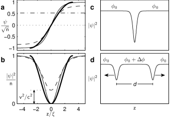
Figure 1: Solitons and matter-wave interference fringes. (a) The order parameter near the transition from interference fringes to solitons. The bold solid curve depicts an interference fringe with $\lambda=4\pi\xi$. The narrow solid curve shows a soliton with $v=0$. Both of these order parameters are real. The dashed (dash-dotted) curve indicates the real (imaginary) part of a grey soliton, with $v=0.53c$. (b) The density associated with the curves of part (a). (c) The initial density and phase of our experiment, created by density engineering. (d) The density and phase of two counterpropagating solitons.

Solitons can also be created by phase engineering Burger et al. (1999); Denschlag et al. (2000). There is a phase step $\Delta\phi\leq\pi$ across the grey soliton, given by $\Delta\phi=2\cos^{-1}(v/c)$. By imposing this phase step, the density profile will evolve into that of a soliton. We can understand this process by considering the current density $\mathbf{J}=(\hbar/m)n\nabla\phi$. By imposing the phase step, this current density is significant in the region of the step only. This corresponds to a divergence in the flow field, $\nabla\cdot\mathbf{J}=\partial J_{z}/\partial z\neq 0$. Since the condensate obeys the continuity equation $\nabla\cdot\mathbf{J}=-\partial n/\partial t$, The divergence depletes the density, forming the soliton minimum.

We use density engineering to form solitons, a complementary technique to phase engineering. We impose the density profile, and the phase evolves into that of a soliton. The process is illustrated in Fig. 1d which shows two solitons separated by a distance $d$. They are moving in opposite directions, with the corresponding opposite phase steps. Our initial configuration shown in Fig. 1c can be thought of as the $d=0$ case of Fig. 1d. Our initial configuration thus corresponds to two overlapping, counterpropagating solitons.

In a one-dimensional (1D) condensate, solitons are stable objects. In three dimensions however, grey solitons were seen to decay irreversibly into vortex rings via the snake instability Anderson et al. (2001); Dutton et al. (2001); Kadomtsev and Petviashvili (1970); Jones et al. (1986); Josserand and Pomeau (1995); Feder et al. (2000); Brand and Reinhardt (2002); Theocharis et al. (2003), which was originally measured in optical solitons Mamaev et al. (1996). We find a very different, stable behavior shown in Fig. 2 by a simulation of the 3D Gross-Pitaevskii equation (GPE) Pitaevskii and Stringari (2003). The soliton evolves into a vortex ring, which subsequently evolves back into a soliton. This process repeats itself many times with a period of 7–8 ms. We call this a “periodic soliton/vortex ring”. The periodic soliton/vortex ring is stable, surviving the reflection from the end of the condensate, as well as the subsequent collision in the middle of the condensate. The periodic soliton/vortex ring has a constant phase step ($0.7\pi$ for our experiment), as shown in Fig. 2j, k.

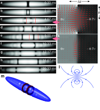
Figure 2: Simulation of the periodic soliton/vortex ring. This simulation shows $3\times 10^{4}$ atoms. (a)–(i) Slices of the condensate. The shades of grey indicate the density. (a) The condensate during the turn-off of the barrier. (b), (e), (h) The soliton stage of the periodic soliton/vortex ring. (c), (g), (i) The vortex ring stage. The axis of the 2 counterpropagating vortex rings is horizontal in the image. The slice of the vortex ring appears as two dark spots, separated vertically. (d), (f) The transitions between the soliton and vortex ring stages. (j) The shades of grey indicate the phase, and the red vectors indicate $\mathbf{J}$. The image is an enlargement of the area between the red lines of part (c). The values $0$ and $-0.7\pi$ indicate the phase on either side of the phase step. (k) As in part (j), except that the enlargement refers to part (e). (l) An illustration of the slice of a vortex ring in an infinite, homogeneous condensate. (m) An illustration of the 2 counterpropagating vortex rings of part (c), showing a surface of constant density (blue) as well as a surface of constant flow speed (red).

First, we will understand the evolution of the soliton into a vortex ring in terms of conservation of energy. Due to the higher density near the center of the condensate, the soliton moves fastest in this region Denschlag et al. (2000). This causes the soliton to curve Denschlag et al. (2000), as shown in Fig. 2f. Due to the curvature, the area of the soliton has increased, corresponding to an increase in the soliton energy. To conserve the energy of the soliton, the increase in area must be compensated by an increase in $v$, by equation 1. This corresponds to a reduction in the depth of the soliton, as shown in Fig. 1b. The soliton thus moves with ever-increasing speed and decreasing depth, until the density minimum vanishes altogether, leaving a vortex ring, as shown in Fig. 2c, g, and i. The appearance of the vortex ring does not violate Kelvin’s theorem (conservation of circulation), because the vortex core can enter and exit the condensate via the nearby boundary Donnelly (1991).

The fate of vortex rings in a quantum fluid is a long-standing field of study Donnelly (1991); Rayfield and Reif (1964). In superfluid ⁴He at non-zero temperatures, it was suggested that the radius of a vortex ring shrinks in time due to dissipation, until it evolves into a roton. We can understand the very different evolution of our vortex ring into a soliton in terms of conservation of mass. We consider a vortex ring in an infinite homogeneous condensate Pitaevskii and Stringari (2003); Guilleumas et al. (2002), as illustrated Rayfield and Reif (1964) in Fig. 2l. The density is constant in time, maintained by the zero divergence of the flow ($\nabla\cdot\mathbf{J}=0$). In other words, after the flow traverses the center of the vortex ring from right to left, it returns to the right outside the vortex ring. In contrast, our vortex ring is close to the edge of the condensate, as shown in Fig. 2c, g, and i. The flow lines therefore have no return path to the right side, causing $\nabla\cdot\mathbf{J}\neq 0$. The divergence depletes the density, forming the soliton minimum. This situation is very similar to that of phase engineering of a condensate described above. In fact, the vortex ring has a phase step, as shown in Fig. 2j. The phase step occurs on a length scale $\Delta z$ on the order of the radius of the vortex ring, which is also the radius $R$ of the condensate. Thus, for creating solitons from vortex rings, $R$ should not be too much larger than $\xi$. This can also be understood energetically. The periodic soliton/vortex ring requires that the soliton and the vortex ring have the same energy. The ratio of these energies contains a factor of $R/\xi$, placing an upper limit on $R$. By the GPE simulation, we find that the vortex ring evolves into a soliton for $R\leq 13\xi$. This requirement implies that the number of atoms in the condensate should not be too large. For our trap frequencies for example, simulations show the periodic soliton/vortex ring for $N\leq 7\times 10^{4}$.

Our experimental apparatus is basically described in Ref. Levy et al. (2007). After reaching BEC, the trap frequencies are adiabatically reduced by half in 350 ms to 117 Hz and 13 Hz in the radial and axial directions, respectively. The resulting condensate contains $1\times 10^{4}$ or $3\times 10^{4}$ ⁸⁷Rb atoms, as specified in the captions of Figs. 3 and 4. The condensate with $3\times 10^{4}$ atoms has $\mu/h=580\,\text{Hz}$ ($h$ is Planck’s constant), corresponding to a minimum healing length of $\xi=0.32\,\mathrm{\mu m}$, which is found at the center of the condensate. The healing length is larger at the lower densities found away from the center. The radii of this condensate are $89\xi$ and $R=10\xi$ in the axial and radial directions respectively. The condensate with $1\times 10^{4}$ atoms has even larger $\xi$ and smaller $R$.

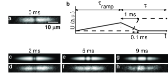
Figure 3: In-situ images of the vortex rings and solitons. The experimental parts of the figure show averages of 2 to 6 destructive phase contrast images, employing small detuning. The condensates contain $1\times 10^{4}$ atoms. (a) The initial condition with the barrier on. (b) The height of the barrier as a function of time (not to scale). The solid curve corresponds to density engineering of solitons. The dashed curve corresponds to the creation of sound pulses. (c) Simulation of the initially formed pair of solitons at $\tau=2\,\mathrm{ms}$. This is an integrated image which includes finite resolution and depth-of-field. (d) In-situ image of the two counterpropagating solitons at 2 ms. (e) Simulation of the vortex ring stage at $\tau=5\,\mathrm{ms}$. This is an integrated image which includes finite resolution and depth-of-field. (f) In-situ image of two counterpropagating vortex rings at 5 ms. (g) Simulation of the soliton stage at $\tau=9\,\mathrm{ms}$. This is an integrated image which includes finite resolution and depth-of-field. (h) In-situ image of two counterpropagating solitons at $\tau=9\,\mathrm{ms}$.

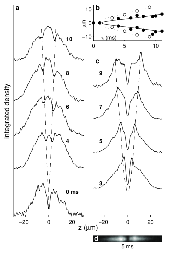
Figure 4: The speed of the periodic soliton/vortex ring. The condensates contain $3\times 10^{4}$ atoms. (a) Integrated profiles of the periodic soliton/vortex ring. Each profile is an average of several images, except for the 0 ms profile. The dashed curves are the result of the simulation. (b) Closed circles indicate the position of the periodic soliton/vortex ring as a function of time. Open circles indicate the position of the sound pulses. The solid and dotted curves are simulations of the periodic soliton/vortex ring and sound pulses, respectively. (c) The sound pulses. Each profile is an average of several images. The dashed curves indicate the simulation. (d) Two counterpropagating sound pulses at 5 ms.

Density engineering is performed by a laser beam, blue detuned by 6 nm from the 780 nm resonance. The condensate is split in the radial direction by the highly elongated laser beam with an axial diameter of $4.4\xi$ ($1.4\,\mathrm{\mu m}$). By the 1D GPE simulations of Ref. Carr et al. (2001), as well as our 3D GPE simulations, this diameter of roughly $4\xi$ is the maximum which will create a single pair of solitons.

We adiabatically ramp up the laser barrier in $\tau_{\mathrm{ramp}}=200\,\mathrm{ms}$ to a height $U=h(3000\,\mathrm{Hz})$, creating a BEC with a density minimum, as shown in Fig. 3a. The potential is then rapidly turned off in 1 ms, resulting in the initial condition illustrated in Fig. 1c. This sequence is indicated by the solid curve in Fig. 3b. As seen in Fig. 3d, one can distinguish the two counterpropagating solitons after 2 ms, which result from the interference between the two condensates of Fig. 3a, colliding with low energy. Figure 3d corresponds to Fig. 1d. Figure 3c shows the simulation at 2 ms with imaging effects, including integration of the density perpendicular to the image, finite resolution, and finite depth of field. The experiment (Fig. 3d) is seen to agree well with the simulation (Fig. 3c).

After a time $\tau=5\,\mathrm{ms}$, we obtain in-situ images of the pair of counterpropagating vortex rings of the periodic soliton/vortex ring, as shown in Fig. 3f. In the image, the two vortex rings are seen as weak density minima. Again, good agreement is seen with the simulation of Fig. 3e. After each of the two vortex rings has evolved back into a soliton, we image the soliton stage at $\tau=9\,\mathrm{ms}$ as shown in Fig. 3h. Two strong, slit-like solitons are seen. We find that the solitons are more visible for the small atom number shown in the figure. Good agreement with the simulation of Fig. 3g is seen.

In order to measure the speed of the periodic soliton/vortex ring, we observe its position as a function of time, as shown in the integrated profiles of Fig. 4a, and the filled circles of Fig. 4b. We see that the speed (the slope) is approximately constant in time, and is therefore the same for the soliton stage and the vortex ring stage. The speed is observed to be $v=0.66\pm 0.08\,\mathrm{mm\,s^{-1}}$, for $N=3\times 10^{4}$. The simulation gives the same results qualitatively and quantitatively, as indicated by the dashed and solid curves of Fig. 4a, b. This speed is of the same order of magnitude as the speed $v\approx(\hbar/2mR)\ln(1.59R/\xi)\approx 0.3\,\mathrm{mm\,s^{-1}}$ predicted for a vortex ring in an infinite, homogeneous condensate Pitaevskii and Stringari (2003); Donnelly (1991); Rayfield and Reif (1964).

The speed of a grey soliton is less than $c$, so it is interesting to compare the speed of the periodic soliton/vortex ring to $c$. We measure $c$ by the technique of Ref. Andrews et al. (1997b). Specifically, we rapidly turn on the barrier in $100\,\mathrm{\mu s}$ and leave it on as indicated by the dashed curve of Fig. 3b, creating two counterpropagating sound pulses, as shown after 5 ms in Fig. 4d. The profiles of Fig. 4c and the open circles of Fig. 4b show the position of the sound pulses as a function of time, giving $c=1.24\pm 0.07\,\mathrm{mm\,s^{-1}}$, which agrees with the theoretical value Zaremba (1998) of $c=\sqrt{\mu/2m}=1.15\pm 0.09\,\mathrm{mm\,s^{-1}}$. The dotted and dashed curves of Fig. 4b, c show the results of the GPE simulation, which agree well with the experiment. We thus find that the periodic soliton/vortex ring moves slower than the speed of sound, at $v=0.53c$.

In conclusion, we have achieved density engineering of a pair of counterpropagating grey solitons, which are the result of a low-energy collision between 2 BEC’s. The close relationship between solitons and matter wave interference fringes elucidates the quantum mechanical nature of solitons in a BEC. Due to the inhomogeneous nature of the narrow condensate, each soliton evolves into a periodic soliton/vortex ring. We explain this evolution in terms of conservation of mass and energy. Since vortex rings and solitons can be considered to be quasiparticles Jones et al. (1986); Pitaevskii and Stringari (2003); Donnelly (1991), perhaps the periodic soliton/vortex ring could additionally be described as a Rabi oscillation between these quasiparticle states. Such a Rabi oscillation is seen in optics, between two soliton states Snyder et al. (1995). As a macroscopic non-linear entity, the periodic soliton/vortex ring has the unusual property that it oscillates between two qualitatively different forms. This presents a puzzle to all branches of science, to categorize this effect by finding other systems with an oscillating nature.