Energetic Analysis of Magnetic Transitions in Ultra-small Nanoscopic Magnetic Rings
Abstract
In this article, we report on experimental and theoretical investigations of magnetic transitions in cobalt rings of size (diameter, width and thickness) comparable to the exchange length of cobalt. Magnetization measurements were performed for two sets of magnetic ring arrays: ultra-small magnetic rings (outer diameter 13 nm, inner diameter 5nm and thickness 5 nm) and small thin-walled magnetic rings (outer diameter 150 nm, width 5 nm and thickness 5 nm). This is the first report on the fabrication and magnetic properties of such small rings. Our calculations suggest that if the magnetic ring’s sizes are comparable to, or smaller than, the exchange length of the magnetic material, then only two magnetic states are important - the pure single domain state and the flux closure vortex state. The onion-shape magnetic state does not arise. Theoretical calculations are based on an energetic analysis of pure and slightly distorted single domain and flux closure vortex magnetic states. Based on the analytical calculations, a phase diagram is also derived for ultra-small ring structures exhibiting the region for vortex magnetic state formations as a function of material parameter.
pacs:
75.75.+a, 81.16.-c, 75.60.EjI INTRODUCTION
In recent times, the magnetic ring geometry has been extensively studied, mostly because of its possible applications in magnetic memory devices. The application in memory devices is mostly driven by the fact that near zero field value, a narrow nanoscopic magnetic ring forms a flux closure vortex magnetic state.Yoo, et al. (2003), Klaui, et al. (2003), Natali, et al. (2002) A magnetic ring in vortex state has zero total magnetization and therefore each ring in an array acts like an individual memory element. Ring geometry is used in atleast one current design of magnetic random access memory (MRAM).Zhu, et al. (2000)
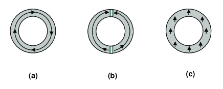
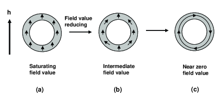
In addition to the vortex magnetic state, a small magnetic ring also forms two other stable magnetic states: ”onion state”, characterized by the presence of two head-to-head domain walls, and single domain (SD) state, as shown in Fig. 1.Rothman, et al. (2001) However, we have found that if the ring sizes are sufficiently small then onion magnetic state has higher energy and does not arise. Therefore, magnetic transition processes in such ultra-small rings involve only two magnetic states: saturating SD state and flux closure vortex state. These conclusions are based on the calculation of total magnetic energies for various possible magnetic states and on the measurement of magnetization as a function of applied field.
Because of the circular geometry of rings, shape anisotropy is absent and also if the parent magnetic material is of polycrystalline origin then magnetocrystalline anisotropy is limited to random grains and can be ignored also.Sko Therefore in zero field the only competing energy terms in the case of polycrystalline magnetic rings are magnetostatic energy and quantum mechanical exchange energy.Cowburn, et al. (2000), Aharoni, et al. (1992). Exchange energy favors the parallel alignment of spins while the magnetostatic energy favors the circular magnetization.
If the ring’s sizes (diameter, thickness and width) are comparable to the characteristic length (exchange length) of the parent magnetic material then the magnetic transition processes are expected to be different from those in relatively larger size nanoscopic rings ( 100 nm). In this new geometrical regime, it is reasonable to assume that the magnetization vector remains confined in the plane of the ring. In this article, we are presenting the study of magnetization and magnetic transitions in ultra-small polycrystalline magnetic, Co, rings of sizes comparable to the exchange length of Co (ex = 3.8 nm).Coe For the first time, magnetic rings are studied at such an unprecedented small length scale.
The magnetic rings are fabricated using copolymer template, angular metal evaporation and ion-beam etching technique. Using this fabrication technique, we have been able to fabricate arrays of rings at two geometrical scales: ultra-small rings with outer diameter 13 nm, ring width 4 nm and thickness 5 nm and small rings with outer diameter 150 nm, ring width 5 nm and thickness 5 nm. The latter are small rings with a thin wall. Magnetization measurements are carried out for arrays of both ultra-small and small rings. Experimental data are explained by detailed theoretical calculations for these rings. The theoretical calculations are based on the energetic analysis of possible magnetic states with the underlying assumption that only the lowest energy magnetic states will be excited. Different magnetic states in a ring structure are obtained using reasonable models of magnetization distortion on the ring’s circumferences.Dee
II FABRICATION PROCEDURE
Recently small ferromagnetic rings have been fabricated by electron beam lithography,Yoo, et al. (2003), Heyderman, et al. (2003) evaporation over spheresZhu, et al. (2004) and other methods.Hobbs, et al. (2004), Kosiorek, et al. (2005) Our nanoring fabrication technique is described in detail in an earlier work.Singh et al. (2008) The fabrication process for both ultra-small and small rings with thin wall (arms) involve the creation of nanoporous polymer templates, angular deposition of desired material, Co, onto the wall of the pores and ion-beam etching technique to remove undesired material from the top as well as bottom of the template. In the case of ultra-small rings, the template is created from a self-assembled diblock copolymer filmAlbretch et al. (2004) while for small rings, the template is created by electron-beam lithography techniqueBal et al. (2002) out of the 40 nm thick copolymer film PMMA [poly(methyl-metha-acrylate)]. The diblock copolymer film has the pore size of 13 nm on the average and thickness 36 nm. The lattice separation between pores is about 28 nm. In the case of copolymer PMMA film, the pore size is 150 nm and the separation between pores (center-to-center distance) is 350 nm. The angular deposition of desired material onto the wall of the nanopores is the most critical step of this fabrication scheme and it depends on the critical deposition angle, c. In our experiment = 13 nm and = 36 nm for the fabrication of ultra-small rings and = 150 nm and = 40 nm for small rings, resulting in the critical angles of c 20o and 75o respectively. Angles of = 23o and 75o were chosen for the fabrication of ultra-small and small rings respectively. The thickness of deposited Co material on nanopores varies in the range of 4-5 nm (based on QCM reading). After material deposition, calibrated ion-beam etching is used to get the desired thickness of both ultra-small and small rings. The desired resulting thicknesses of both ultra-small and small rings are 5 nm.
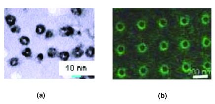
After ion-beam etching, the small ring samples are rinsed in acetone solvent to remove the remaining polymer residues and are characterized by field emission scanning electron microscope (FESEM) (Figure 2). Structural characterization of ultra-small rings is done using tunneling electron microscope (TEM) (Figure 2). Sample preparation of ultra-small rings for TEM imaging involved the transfer of ring templates onto an electron transparent substrate. It is a difficult process and can be found in detail somewhere elseSingh et al. (2008). For the magnetic measurement process, ultra-small rings were not transferred on electron transparent substrate.
III MAGNETIZATION MEASUREMENTS AND DATA ANALYSIS
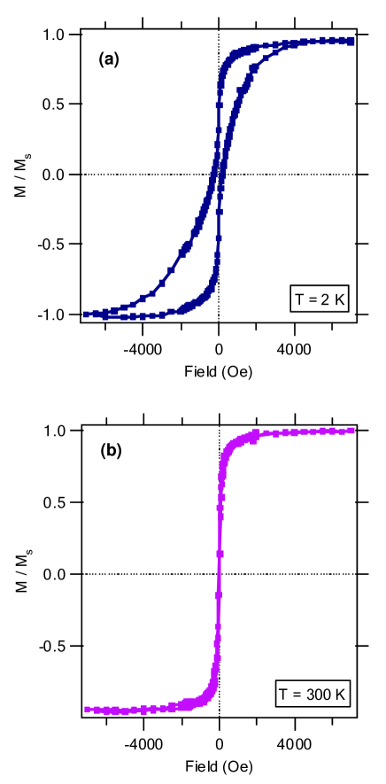
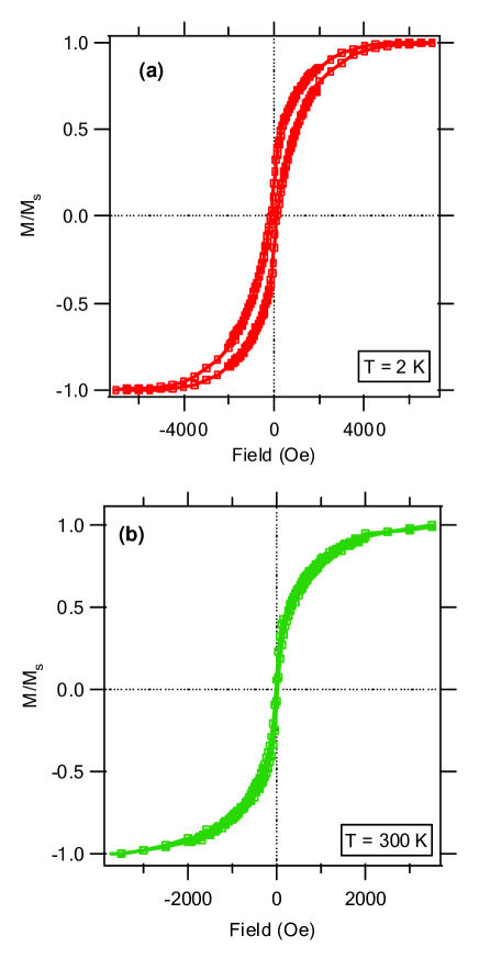
Magnetic measurements of ultra-small and small ring arrays were carried out in a SQUID magnetometer with base temperature 1.8 K and field applied in-plane of the ring. Figure 3 and 4 shows magnetization measurements for arrays of ultra-small and small rings respectively, after the subtraction of a linear diamagnetic background. As we can see in the low temperature in-plane magnetization data for both ultra-small and small rings, the width of the hysteresis curve is smaller near zero field value than near the saturation which is similar to the magnetic transition in nanoscopic narrow rings.Klaui et al. (2004) In relatively larger size nanoscopic rings, it is observed that the magnetic state is single domain (SD) state at saturating field value and as the field is decreased, the ring’s magnetic state forms an ”onion-shape”, near zero field value, and finally transforms to flux closure vortex state (Figure 1).Natali, et al. (2002), Zhu, et al. (2000) It also depends on the ring’s width, diameter and ferromagnetic exchange length.Li, et al. (2001)
To have a complete understanding of these magnetic transition phenomena, one needs to solve the following integro-differential equation:Bro , Aha
| (1) |
where is the radial co-ordinate, is magnetic pole density (depending on azimuthal position ), the kernel is an explicit but complicated function involving and and is the direction of applied magnetic field. By solving these integro-differential equations, we can get the functional (, ) and since () = , explained later, (here we have taken = 1 just for the sake of simplicity), so we can get (magnetization) as a function of (dimensionless magnetic field). This is not an easy task. Another approach is reverse approach.
In this approach, a reasonable model for magnetization distribution on ring’s circumference is assumed in zero field value and total energy is calculated for different possible magnetic states, starting from the first principle. For any shape of body, those magnetic configurations which are energetically favored are dominant in determining the magnetic behavior.Rothman, et al. (2001) In general, the magnetic state of a ring will be determined by the competition between exchange energy, magnetostatic energy, Zeeman energy and magneto-crystalline energy. The exchange energy contribution favors the parallel alignment of the local magnetization m over the entire body while magnetostatic energy favors configurations where the magnetization follows a closed path inside the body, so that no net magnetic moment is produced.
Before considering the magnetization distributions on the ring’s circumference in detail, we first calculate the energies of the uniformly magnetized SD, flux closure vortex and onion states near zero field (Figure 1). For this purpose, first we consider ultra-small ring. Since the thickness (5 nm) and width (4 nm) of the ultra-small ring are comparable to the exchange length of Co material (ex = 3.8 nm),Coe magneto-crystalline anisotropy can be ignored for simplicity. For an ultra-small ring, the energetic analysis described below shows that only single domain and vortex states are of significance at fields near zero; the energy of the onion state lies far above. An important underlying assumption in the calculation of energy is that since the thickness and width of the ring are comparable to the exchange length for cobalt, there is no variation of magnetization along the symmetry axis (easy axis), of the ring i.e. magnetization pattern is purely two-dimensional in nature. Recently other authorsKravchuk, et al. (2006), Landeros, et al. (2007) have found that the variation of magnetization along the symmetry axis in the relatively larger size magnetic rings leads to triple point behavior, separating SD, vortex and onion magnetic states as a function of material’s properties, in phase diagram. We have discussed these results later in the discussion section.
In dimensionless form, the free energy for a magnetic system of volume is given by,Ber
Here m = M/s and a = a/s are dimensionless magnetic fields. a is the applied magnetic field, and M is the magnetic field produced by the magnetization of the sample, which has saturation magnetization s. = 21/0s2 = an/s, where 1 is the first crystalline anisotropy constant (which will be taken to be zero for simplicity). The exchange length ex = (2/0s2), where is the exchange stiffness constant. For the uniformly magnetized SD state, the exchange energy is zero and the total energy is the sum of the magnetostatic and Zeeman contributions.
| (2) | |||||
| (3) |
In the above equation, the dimensionless magnetostatic energy m= 0.20 was obtained by numerical integration. Numerical integration for magnetostatic energy is carried out by assuming the ring’s inner and outer surfaces as two oppositely magnetic charged ribbons separated from each other by the width of rings. Thickness of that ribbon is 5 nm (ring’s thickness). We write the magnetostatic potential at an arbitrary point, in the region between ribbons, and then numerically integrate it over the volume of the ring.
For the vortex state, the magnetostatic, domain wall and Zeeman energy contributions are all zero, so the total energy is solely exchange energy.
| (4) | |||||
| (5) |
To calculate the energy of the onion configuration, we separate it into two parts: the ring arms and the domain walls (DW). The contributing energy terms are exchange, Zeeman and magnetostatic. Exchange energy is proportional to m2, so the vortex and the ring arms of the onion state have the same exchange energy. The energy of onion magnetic state is
where 1 is the inner radius, 2 is the outer radius. Both m(ringarms) and DW are positive: each increases the total energy of the onion state.

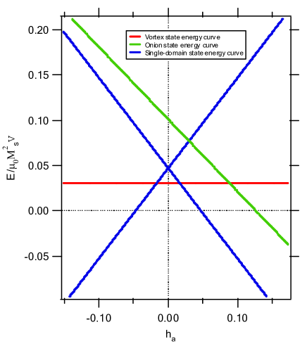
The energies of the SD and vortex states, together with a lower limit of the onion state energy, are plotted as functions of the dimensionless applied field a in Figure 5. The lower limit is obtained by neglecting the domain wall and magnetostatic terms. This figure suggests that the energy landscape has three local minima and that these three magnetic states have locally minimal energies. According to this energy plot, it is inferred that SD state is always lowest in energy. Vortex and onion magnetic state does not excite. Hence the corresponding magnetic hysteresis curve would be a one step transition, from one SD state to another SD state of opposite polarity. This is not exactly the experimental data for ultra-small magnetic rings (Fig. 3).
As mentioned previously, rings are made of polycrystalline Co material. In the case of polycrystalline material, random anisotropies of grains play a crucial role in determining the intergranular interaction. If the grains are small then intergranular interactions becomes more dominating than interatomic exchange interaction and thus lower the exchange length values. As a result, the energy of vortex magnetic state would be smaller. In that case, a transition from saturating SD state to vortex state, near zero field value, is quite likely.
Depending upon the polycrystalline exchange length of Co, magnetic transition in ultra-small ring can occur from SD state to vortex state via the distortion of pure SD state, or from the pure vortex state to pure SD state via the distortion of vortex state. An important question arises then: are these intermediate (distorted) magnetic states stable i.e. lower in energy compared to pure SD and vortex states respectively. It is found that small distortions of the SD state increases its energy. In the following section, detail calculation and results are explained for distorted SD and vortex state.
IV DISTORTED SINGLE DOMAIN AND VORTEX STATES
For an ultra-small ring, at very high field the magnetic state is saturated single domain. When the field is reduced from the saturation value, SD state is supposed to distort and eventually attains a vortex configuration near zero value of field, depending on the polycrystalline exchange length of Co material. A schematic description of this phenomenon is shown in Figure 6. In this figure, we call the magnetic state at intermediate field value as the ”distorted single domain state”. If the distorted SD state is unfolded into one dimension, then the envelop over magnetic spin shows an oscillatory character, as shown below in Figure 7a.
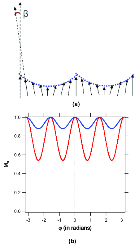
In Figure 7a, is the angle between an arbitrary spin and the applied field axis. An arbitrary spin is represented by the angle on the circumference of ring. So varies between 0 and 2. The very important underlying assumption in this model is the slow variation of angle over the circumference of ring in the distorted single domain magnetic state. Now we seek a function = (), which will give us magnetization distribution as shown in the profile in Figure 7a. By keeping in mind that the profile of magnetic spins shows oscillatory behavior, we make an assumption for the variation of angle as a function of as:
| (6) |
| (7) | |||||
| (8) |
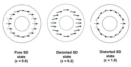
where is the distortion coefficient and is the direction of externally applied magnetic field. Figure 7b shows the variations of x as a function of for two different distortion parameters of = 0.2 and 0.5. It is a reasonably good approximation (if not exact) for magnetization distribution. For different values of distortion coefficients, the distortion of magnetic spins on the circumference of a ring is shown in Figure 8.
In single domain state, () = 0, so = 0, which is same as in Figure 8. On the other hand if = 1 then not all the spins are aligned along the magnetic field. Spins which are not aligned along the magnetic field appear to be distorted from their original direction while other spins are still aligned along the magnetic field direction. We call this state as distorted SD magnetic state. At zero applied field, the total dimensionless energy, g(), of distorted SD state is the sum of two terms:
g() = gex()+gms()
As mentioned in the previous section, we reasonably ignore crystalline anisotropy term in total energy calculation.
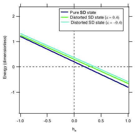
Starting from the first principle (as described in previous section), exchange energy and magnetostatic energy are calculated as a function of distortion coefficient () for ultra-small ring geometry. All the three energy terms, exchange energy, magnetostatic energy and total energy are plotted in Figure 11 as a function of distortion coefficient . In this figure, if all the spins are aligned in one direction i.e. no distortion ( = 0) and thus creating a SD state then exchange energy is minimum (zero) but magnetostatic energy is maximum. As the distortion is increased so that spins are not aligned in one direction and therefore it is no longer a pure SD state then exchange energy also increases for increasing values of but magnetostatic energy shows different trend. Magnetostatic energy starts decreasing for increasing values of distortion coefficient but for higher distortions ( 1.2) the magnetostatic energy starts increasing again. The total energy of distorted SD state increases with increasing value of .
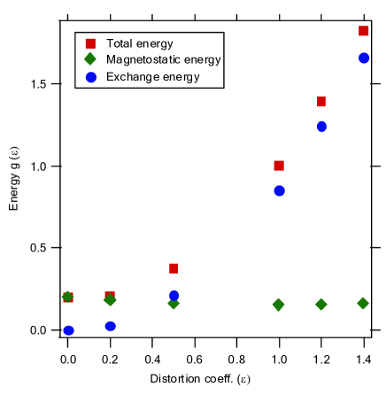
Although magnetostatic energy decreases for increasing values of but it does not affect the overall increase of total energy. This happens because of larger exchange energy contributions as the pure SD state becomes more and more distorted. Thus we conclude that for perturbations of this particular form, the minimum energy state is still of pure SD state. It means, for this model function ( = ()), pure SD state has lower energy than distorted single domain states in zero field. Since exchange and magnetostatic energies are independent of field, so even in the presence of field pure SD state is still of lowest energy as compared to distorted SD states. For different values of (pure SD and perturbed SD states), total energy of an ultra-small ring are plotted in Figure 10 as a function of applied magnetic field. Here it is important to mention that the distorted SD state with = 1.0 is not an ”onion” magnetic state. The onion state will have extra energy as a result of formation of domain walls. Our calculations suggest that distorted states with greater than zero are higher in energy than the pure SD state, even though states with different have different sensitivities to applied field (i.e. Zeeman energy depends on ). Perhaps the magnetization does distort, but to some other shape, that we did not take into account.
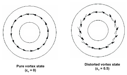
Another possible magnetic transition involves the magnetic state of ultra-small ring is already a vortex state near zero value of field and it makes transition to saturating single domain state via some intermediate magnetic state. For this purpose, we consider another realistic model that involves a vortex distortion constant, v. In this model, vortex magnetization state is given by,
| (9) |
once again () is the angle between the direction of the magnetization and the field direction (applied along the x-axis). Different vortex states are shown in Figure 11 for the vortex distortion constants, v , of 0 and 0.5. For the vortex distortion constant value of v = 0 means no distortion and in that case, () = /2 + . We see that for v = 0, magnetization configuration is indeed of pure vortex state. Again, the total energy of the ultra-small ring in zero field consists of exchange and magnetostatic energy terms (ignoring the magneto-crystalline anisotropy energy term in the total energy calculation). The first principle calculation of exchange energy for distorted vortex states as a function of v is given by the following equation:
| (10) |
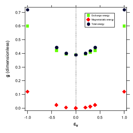
Magnetostatic energies for distorted vortex states are calculated by numerical integrations (as explained previously). The energies for distorted vortex states as a function of vortex distortion constant v are plotted in Fig. 12, in zero applied field. In this figure, the pure vortex state is indeed the lowest energy state in zero field because of the dominance of exchange energy term in the total energy. However as we will see in the following paragraph, this is not the case in the presence of field.
In the presence of field, the total energy consists of three terms:
g(v) = gex(v) + gms(v) + gzeeman(v)
The calculated Zeeman energies for distorted vortex states is given by:
The Zeeman energy is proportional to the applied field a . So at first instance it appears that pure vortex state will always remain the magnetic state of lowest energy but at the same time we see from the Zeeman energy expression that the slope of the Zeeman energy curve depends on the distortion parameter v. Total energy, including the Zeeman energy, for pure as well as distorted vortex states (distortion parameters v = 0.2, 0.3) are plotted in Figure 13 as a function of applied field. Some very interesting behaviors are observed in this figure.
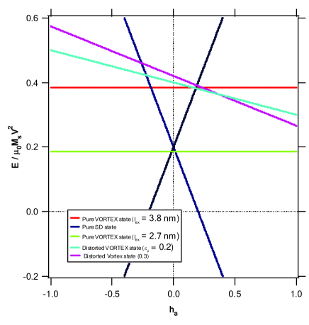
Near zero field values, pure vortex state is still the lowest energy state. At a field of 0.2 or so the state with distortion v = 0.2 crosses over to become lower than the state with distortion v = 0.0. At a somewhat higher field the green state with distortion parameter v = 0.3 becomes the one with lowest energy. This is not exactly the case for distorted SD states (Figure 10), as discussed earlier. In the case of single domain states, pure SD state remains lowest in energy as the applied field is changed. Therefore distorted single domain states can be ignored in considering the magnetic transition for ultra-small rings. Thus there are three important states to consider: pure SD state, pure vortex state and distorted vortex state. In Figure 13 we have plotted all these energies as a function of applied field. It is observed that pure SD state is always the lowest energy state. In this figure, an additional vortex state, arising for a lower exchange length value (ex = 2.7 nm) of polycrystalline Co material, is also plotted. This vortex curve intercepts the pure SD curves at dimensionless a = 0.01. The implications are explained in the following section.
V DISCUSSION
Based on the above analysis and crystalline exchange length value (ex = 3.8 nm), the magnetization hysteresis curve for ultrasmall ring would be one step transition at zero field which is not quite the experimental data (Figure 3). The experimental hysteresis curve shows zero magnetization at a = 0.01 (equivalent to 90 Oe of applied magnetic field). Now, as mentioned previously, the rings are poly-crystalline, resulting in an effective exchange length that is smaller than the 3.8 nm bulk value used in the calculations. For a given geometry, the energy of a vortex at zero field is proportional to the square of the exchange length, while the energy of an SD state is independent of the exchange length. If we consider an exchange length of 2.7 nm for the polycrystalline Co material then the vortex state has the lowest energy at zero field and is degenerate with an SD state at fields of about a = 0.01 (Figure 13). Theoretically, the corresponding hysteresis curve would be two steps separated by a short plateau of width about 0.02, as shown in Figure 13. This provides a qualitative explanation of the experimental magnetization data of ultra-small magnetic rings at = 2 K.
From this analysis we can conclude that near zero field, ultra-small rings will be in either a single domain state or a vortex state, depending upon the polycrystalline exchange length value. The onion state is not expected to play a role.
Now we check the validity of above analysis for ultra-small magnetic rings in relatively longer geometrical regime of small ring of thin wall (outer diameter 150 nm). As mentioned in the fabrication section, small ring’s width and thicknesses are comparable to that of ultra-small rings and therefore to the characteristic length of Co. However, the outer diameter of small rings are an order of magnitude larger than the diameter of ultra-small rings. The vortex energy and magnetostatic energy depends on the outer diameter of the ring geometry. Based on the first principle calculation, the three possible energy terms SD, onion and vortex magnetic state are plotted as a function of magnetic field in Figure 14. As inferred from Fig. 14, in this case also the onion state does not arise and the magnetic transition occurs between two SD states via the formation of vortex magnetic state. Interestingly, in the case of thin wall small rings vortex magnetic state arises even for the exchange length value of ex = 3.8 nm. The reason behind this is the dominance of magnetostatic energy term in the overall energy counting. Therefore as the lateral size of a ring increases, magnetostatic energy starts dominating over the exchange energy term. The experimental (in-plane) magnetization data (at 2 K) for small rings, Figure 4, does not seem to be in good agreement with Fig. 14. Although the magnetic transition starts occurring around 1000 Oe of field value but the curvature of magnetic transition is very large, in terms of field, indicating that the magnetic transition process in small rings may not be as simple. As the overall ring size increases, the magnetostatic energy of the distorted SD states start dominating in the total energy counting and therefore enhances the possibility of interaction between individual ring elements. It leads to magnetocrystalline anisotropy in the ring arrays that we have not taken into account in the calculation. Some authors have calculated anisotropy energy for relatively thicker magnetic rings.Zhu, et al. (2006) More general first principle calculation would be necessary to understand the magnetization reversal in thin wall small rings.
Magnetic measurements at room temperature for both ultra-small and small rings do not show any magnetic hysteresis. At high temperature, thermal fluctuations play dominant role, as compared to the magnetic energy of these rings. This cancels out any remnant magnetization at zero field. Weakly noticeable asymmetricity of magnetization loops for positive and negative fields, in the low temperature magnetic hysteresis curve of ultra-small ring arrays (Fig. 3a), is possibly due to the weak exchange bias phenomena. On the surface of the ring, partial oxidization of Co material into CoO creates an interface of FM (Co) / AFM (CoO) layer, resulting into very weak exchange bias phenomena. A similar behavior has recently been reported in the case of magnetic disk.Sort, et al. (2005)
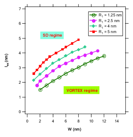
Now we summarize the above analysis for ultra-small ring geometry. Rings made of polycrystalline Co material can have smaller exchange length than the crystalline value. This exchange length, along with the ring’s geometrical parameters, decides which magnetic state has the lowest energy at zero field. Increasing the diameter reduces both the magnetostatic and exchange energies but the exchange energy decreases more rapidly and therefore magnetostatic energy starts dominating as the overall diameter of the magnetic ring increases. For given inner and outer radii difference, there is a value of the exchange length at which the vortex and SD states are degenerate at zero field. We have also drawn a phase-diagram in Figure 15 that shows the value of exchange length, ex as a function of ring width (2 - 1). If the ring’s exchange length is larger than the ordinate of that point, the SD states will be lowest at zero field, otherwise a vortex state will be the lowest. This phase diagram may not be valid for larger size nanoscopic rings. As there is a strong underlying assumption in the above analysis is that the magnetization pattern in the case of ultra-small magnetic ring is purely 2-D. Magnetization vector does not cant-out of the ring’s plane. For an ultra-small ring with width and thicknesses comparable to the characteristic length (exchange length) of the parent magnetic material, this assumption is quite reasonable. As a consequence, we do not observe the ”triple point” – defined as the point where the energies for onion, vortex and uniform out-of-plane magnetization are same – as recently reported by other authors based on theoretical calculations for the ring geometry.Kravchuk, et al. (2006), Landeros, et al. (2007).
Acknowledgements
This project was supported by NSF Grants DMR-0531171, DMR-0306951 and MRSEC.
References
- Yoo, et al. (2003) Y. G. Yoo, et al., Appl. Phys. Lett. 82, 2470 (2003).
- Klaui, et al. (2003) M. Klaui, et al., J. Phys.: Cond. Matt. 15, R985 (2003).
- Natali, et al. (2002) M. Natali, et al., Phys. Rev. Lett. 88, 157203 (2002).
- Zhu, et al. (2000) J. G. Zhu, et al., Jour. Appl. Phys. 87, 6668 (2000).
- Rothman, et al. (2001) J. Rothman, et al., Phys Rev Lett 86, 1098 (2001).
- (6) R. Skomsky, Chapter 10, Spin Elctronics, Springer Publishing Group (2000).
- Cowburn, et al. (2000) R. P. Cowburn, et al., J. Phys.D: Appl. Phys. 33, R1 (2000).
- Aharoni, et al. (1992) A. Aharoni, et al., Phys. Rev. B 45, 1030 (1992).
- (9) J. M. D. Coey, Chapter 12, Spin Elctronics, Springer Publishing Group (2000).
- (10) Deepak Kumar Singh, Ph. D. Thesis 2006, University of Massachusetts Amherst, Available at: http://scholarworks.umass.edu/dissertations/AAI3242328/.
- Heyderman, et al. (2003) L. J. Heyderman, et al., Jour. Appl. Phys. 93, 10011 (2003).
- Zhu, et al. (2004) F. Q. Zhu, et al., Advanced Materials 16, 2155 (2004).
- Hobbs, et al. (2004) K. L. Hobbs, et al., NanoLetter 4, 167 (2004).
- Kosiorek, et al. (2005) A. Kosiorek, et al., SMALL 1, 439 (2005).
- Singh et al. (2008) D. K. Singh et al., Nanotechnology 19, 245305 (2008).
- Albretch et al. (2004) T. Albretch et al., Advanced Materials 12, 787 (2004).
- Bal et al. (2002) M. Bal et al., Appl. Phys. Lett. 81, 3479 (2002).
- Klaui et al. (2004) M. Klaui et al., Appl. Phys. Lett. 85, 5637 (2004).
- Li, et al. (2001) S. P. Li, et al., Phys Rev Lett 86, 1102 (2001).
- (20) ”Micromagnetics”, Interscience Publishers (1963).
- (21) A. Aharoni, Theory of Ferromangetism, Oxford Science Publication (2000).
- Kravchuk, et al. (2006) V. P. Kravchuk, et al., J. Mag. Mag. Mat. 310, 116 (2006).
- Landeros, et al. (2007) P. Landeros, et al., Jour. Appl. Phys. 100, 044311 (2007).
- (24) M. Bertotti, Hysteresis and magnetism, Academic Press (1998).
- Zhu, et al. (2006) F. Q. Zhu, et al., Phys. Rev. Lett. 96, 027205 (2006).
- Sort, et al. (2005) J. Sort, et al., Phys. Rev. Lett. 97, 067201 (2005).
*email: tuominen@physics.umass.edu