The white dwarf population in NGC 1039 (M34) and the white dwarf initial-final mass relation

Abstract

We present the first detailed photometric and spectroscopic study of the white dwarfs (WDs) in the field of the $\sim 225$ Myr old ($\log\tau_{cl}=8.35$) open cluster NGC 1039 (M34) as part of the ongoing Lick-Arizona White Dwarf Survey. Using wide-field $U\!BV$ imaging, we photometrically select 44 WD candidates in this field. We spectroscopically identify 19 of these objects as WDs; 17 are hydrogen-atmosphere DA WDs, one is a helium-atmosphere DB WD, and one is a cool DC WD that exhibits no detectable absorption lines. We find an effective temperature ($T_{\rm eff}$) and surface gravity ($\log g$) for each DA WD by fitting Balmer-line profiles from model atmospheres to the observed spectra. WD evolutionary models are then invoked to derive masses and cooling times for each DA WD. Of the 17 DAs, five are at the approximate distance modulus of the cluster. Another WD with a distance modulus $0.45$ mag brighter than that of the cluster could be a double-degenerate binary cluster member, but is more likely to be a field WD. We place the five single cluster member WDs in the empirical initial-final mass relation and find that three of them lie very close to the previously derived linear relation; two have WD masses significantly below the relation. These outliers may have experienced some sort of enhanced mass loss or binary evolution; however, it is quite possible that these WDs are simply interlopers from the field WD population. Eight of the 17 DA WDs show significant Ca II K absorption; comparison of the absorption strength with the WD distances suggests that the absorption is interstellar, though this cannot be confirmed with the current data.

1. Introduction

This is the fourth installment in a series of papers investigating the white dwarf (WD) content in young open clusters. The primary goal of these studies is to better constrain the integrated mass lost by low to intermediate mass stars during their main sequence and advanced stages of evolution. This mass loss is most commonly represented as an initial-final mass relation (IFMR, e.g., Weidemann, 1977, 2000). Constraining the IFMR is crucial to understanding the chemical enrichment due to stellar mass loss and star formation efficiency in galaxies (Ferrario et al., 2005). The shape of the IFMR has a direct effect on the shape of the WD luminosity function (WDLF), which is commonly used to constrain the age of the Galactic thin disk (e.g., Winget et al., 1987; Harris et al., 2006), the thick disk, the Galactic halo (e.g. von Hippel et al., 2005b), and globular clusters (e.g., Hansen et al., 2002, 2004, 2007).

Much work has been done to constrain the IFMR semi-empirically. The first purely photographic study was done by Romanishin & Angel (1980); spectroscopy of WDs, which is necessary to determine their masses and cooling times, was added to studies of the IFMR in a series of papers by Koester & Reimers (e.g., 1981, 1996). Motivated by this progress, Weidemann (2000) updated his semi-empirical IFMR. More recent work on open clusters by Claver et al. (2001), Kalirai et al. (2005) and Williams et al. (2004a) led Ferrario et al. (2005) to re-determine the empirical IFMR. They found that a linear function adequately described the observational data. More recent purely empirical IFMR determinations (e.g., Williams, 2007; Kalirai et al., 2008) also find the empirical IFMR can be adequately parameterized as a linear function; the slopes derived in these studies are consistent with the slope found by Ferrario et al. (2005).

Another aim of these studies is to more accurately determine the upper limit on the main sequence mass of a star that evolves into a WD. This limit is an important parameter in modeling dwarf galaxy evolution in particular (Dekel & Silk, 1986), as it constrains the amount of energy and matter produced during the evolution of a given stellar population. Recent theoretical studies (Poelarends et al., 2008) of the advanced stages of stellar evolution find that the lower limit on the mass of a solar metallicity star that will ignite carbon burning is $\sim 7M_{\odot}$. Only stars with masses below this limit should be able to form CO-core WDs. Between $\sim 7M_{\odot}$ and $\sim 9M_{\odot}$, stars modeled in Poelarends et al. (2008) ignite carbon but do not ignite neon and oxygen, so that some of them may form ONe-core WDs. These limits have yet to be tested observationally. WD studies to date have investigated WDs with initial masses between $\sim 1.2$ and $6.5M_{\odot}$ (Ferrario et al., 2005; Kalirai et al., 2008). It is important to explore the WD populations of young open clusters with possible massive, still relatively bright WDs for this reason.

A third use of these studies of WDs in young open clusters is to compare cluster ages as determined by main-sequence fitting with WD cooling times (von Hippel et al., 2005a). Consistency of these ages increases confidence in both stellar evolutionary models and WD cooling models. Consistency across a wide range of star cluster ages further increases confidence in studies seeking to derive star-formation history from the WDLF (e.g., Liebert et al., 2005).

Our general approach is to use photometric observations of young clusters in order to select likely WD cluster member candidates based on their location in the color-magnitude and color-color ($U$–$B$ versus $B$–$V$) diagrams for the fields. We then obtain high signal-to-noise spectra of these candidates. With spectroscopy of cluster WD candidates, it is possible to unambiguously determine if the objects are WDs. For the bona fide WDs, we determine the effective temperature ($T_{\rm eff}$) and surface gravity ($\log g$), and from those quantities and WD evolutionary models, we derive the cooling age ($\tau_{\mathrm{W}D}$), mass, and luminosity of each WD. For those WDs with cooling ages less than the cluster age and distance moduli consistent with cluster membership, subtraction of the WD cooling age from the age of the open cluster results in the lifetime of the progenitor star, and stellar evolutionary models can then be used to determine the progenitor star mass.

As part of our ongoing program to identify and spectroscopically analyze the WD populations of open clusters, the Lick-Arizona White Dwarf Survey (LAWDS, Williams et al., 2004a), we have obtained imaging data to identify candidate WDs in NGC 1039 and high signal-to-noise spectra of WDs in the field of NGC 1039.

In this paper, we assume the solar metallicity value of Asplund et al. (2004, $Z=0.013$) and the extinction curve of Rieke & Lebofsky (1985) with $R_{V}=3.1$.

1.1. Previous Studies of NGC 1039

The first study of WDs in NGC 1039 (M34) was done by Anthony-Twarog (1982). In this study, $U\!BV$ photographic plates were used to obtain photometry for stars in the cluster field and to select objects with significant blue color excess. The color-magnitude sequences for WDs derived by Sion & Liebert (1977) and Koester et al. (1979) were compared with these observations. Four objects were found to be close to the WD cooling curves used in color-magnitude and color-color space, and so could be interpreted as being cluster member WDs. The number of field WDs of different apparent $V$ magnitudes expected to appear in the photometry was calculated using the then-current WDLF (Green, 1980). This number of expected field WDs ($\sim 23$ with $V\leq 21$) was, in fact, larger than the number of observed blue objects (11 with $\bv\leq 0.4$), leading to the conclusion that NGC 1039 did not have a significant number of WDs.

A number of recent studies have been done on NGC 1039. Ianna & Schlemmer (1993) present proper motions to determine which objects are cluster members. They determine $(m-M)_{0}=8.28$ and an age of $\log\tau_{cl}=8.40$ using $E(B-V)=0.07$. Meynet et al. (1993) compare new stellar models to previously obtained data. They use $E(B-V)=0.10$ and calculate $(m-M)_{0}=8.34$ and an age of $\log\tau_{cl}=8.25$. Jones & Prosser (1996), again using a proper motion selected sample, use $E(B-V)=0.07$ and obtain $(m-M)_{0}=8.38$ and $\log\tau_{cl}=8.30-8.40$.

The most recent study of NGC 1039 is that of Sarajedini et al. (2004). These authors combine $U\!BV\!RI$ photometry from the WIYN open cluster survey with $J\!H\!K$ photometry from 2MASS to obtain accurate distance estimates. They assume $E(B-V)=0.10$ and $[\mbox{Fe/H}]=+0.07$ and derive $(m-M)_{0}=8.67\pm 0.07$. The spectroscopic metal abundance of NGC 1039 has been determined to be slightly super-solar. Schuler et al. (2003) find $[\mbox{Fe/H}]=+0.07\pm 0.04$, and new work from the WIYN Open Cluster Study finds $[\mbox{Fe/H}]\approx+0.08$ (A. Steinhauer, private communication, 2008). In this paper, we assume solar metallicity for the cluster.

2. Photometric Observations & Analysis

2.1. Photometric Measurements and Calibration

$U\!BV$ imaging of a field centered on NGC 1039, as well as of two fields $25^{\prime}$ to the north and south of the cluster center, was obtained in 2004 September and 2005 December with the KPNO 4m MOSAIC camera. Exposures of 5, 30, and $3\times 120$ s were obtained at the northern field in both $B$ and $V$ and at the central field in $V$; exposures of 5, 30, and $3\times 150$ s were taken at the central field in $B$. We obtained exposures of 5 and 120 s in $B$ and $V$ at the southern field. Exposures of 5, 30, 120, and $3\times 900$ s were obtained in $U$ at the central field; all of these but the 30 s exposure were obtained in the northern field. The southern field was observed with exposures of 15, 120, and $3\times 600$ s in $U$. The northern and southern fields are positioned at very nearly the same right ascension (R.A.) as the central field. Each flanking field overlaps the central field by $\sim 11\arcmin$ on either its northern or southern end. Seeing ranged between $0\farcs 8$ and $1\farcs 0$ in the $V$-band in 2004 September and was $\sim 1\farcs 7$ in the $B$-band in 2005 December.

We reduced the data using the IRAF $mscred$ mosaic reduction package. The data were bias subtracted, trimmed, flat-fielded and projected onto the tangent plane. Object detection and aperture photometry were performed using the DAOPHOT II program (Stetson, 1987); aperture corrections were determined and applied using the program DAOGROW (Stetson, 1990).

Star-galaxy separation was performed by comparing the $V$-band flux in two successively larger apertures for each object: an inner aperture with a radius equal to the full-width half-maximum (FWHM) of the $V$-band point spread function ($\approx 0\farcs\,8$) and an outer aperture with a radius of twice the FWHM. Stars were observed to form a tight sequence with a constant difference in aperture magnitudes of $\approx 0.3$ mag for $V\lesssim 23$; we therefore identified objects with aperture magnitude differences $\leq 0.5$ and $V\lesssim 23$ as point sources. We consider only these point sources in the subsequent analysis.

As the MOSAIC images of NGC 1039 were taken under non-photometric conditions, we calibrated these images using previously obtained $U\!BV$ imaging of the central portion of NGC 1039 taken with the Nickel 1-m telescope at Lick Observatory on 2002 July 6. These images were reduced and aperture photometry was determined for each star. The Nickel imaging was calibrated using standard stars from Landolt (1992). The stars with calibrated Nickel photometry were then used as secondary standard stars for calibrating the MOSAIC imaging.

Calibrations were obtained by solving the following transformation equations for both the MOSAIC and Nickel imaging:

$$\scriptstyle u \scriptstyle= \scriptstyle U+2.5\log t_{exp}+A_{0}+A_{1}(X-1.25)+A_{2}(U-B)+A_{3}(U-B)^{2}$$ (1)

$$\scriptstyle b \scriptstyle= \scriptstyle B+2.5\log t_{exp}+B_{0}+B_{1}(X-1.25)+B_{2}(B-V)$$ (2)

$$\scriptstyle v \scriptstyle= \scriptstyle V+2.5\log t_{exp}+C_{0}+C_{1}(X-1.25)+C_{2}(B-V),$$ (3)

where $u$, $b$, $v$ are total instrumental magnitudes; $U$, $B$, $V$ are standard magnitudes; $t_{exp}$ is the exposure time; and $X$ is the airmass.

Zero points and color terms were calculated for the MOSAIC data; as local secondary standards were used, the airmass terms were not necessary. Values for the transformation coefficients are given in Table 1. The $B$ and $V$ color terms are consistent with average values determined by Massey et al. (2006) for the MOSAIC camera; the $U$-band color terms are not directly comparable because we have chosen a quadratic formula.

We compared our calibrated MOSAIC photometry of 46 objects with that of Jones & Prosser (1996). There is no significant trend in the magnitude of $\bv$ color offset with magnitude or color between the two systems. The mean offset in $V$ magnitude is 0.021, with a dispersion of 0.048. The mean offset in $\bv$ color is 0.008, with a dispersion of 0.050.

The left most panels of Figures 1 and 2 show our final calibrated photometry for the cluster in $B-V$, $V$ and $U-V$, $V$ color-magnitude diagrams. Note that sources with $V\lesssim 13$ are saturated in our photometry. Jones & Prosser (1996) photometry is overplotted in the second left panel in Figure 1 for stars with a high probability of cluster membership ($>67\%$, where probability is determined from their proper motion study).

2.2. WD Candidate Selection

We select WD candidates using photometric criteria based on synthetic evolutionary sequences of WDs kindly provided by P. Bergeron; these sequences represent an extension of those published in Bergeron et al. (1995), including improved color calculations (Holberg & Bergeron, 2006) and the more recent WD evolutionary calculations of Fontaine et al. (2001).

The second right panel of Figure 1 and the middle panel of Figure 2 show isochrones and WD cooling curves adjusted to the cluster’s $(m-M)_{V}$ and $E(\bv)$ using cluster parameters from Jones & Prosser (1996). The right-hand panels of both figures show the same isochrones and WD cooling curves, adjusted using cluster parameters from Sarajedini et al. (2004). The solid isochrones are Padova models for $\log\tau_{cl}=8.35$ (Girardi et al., 2002), interpolated for $Z=0.013$. The dashed isochrones are Yonsei-Yale $\log\tau_{cl}=8.35$, $Z=0.013$ models interpolated from solar-scaled abundance models using the code provided by the Yonsei-Yale Group (Demarque et al., 2004). The dotted isochrone in Figure 1 is the fiducial main sequence of the sub-solar metallicity cluster NGC 2168 given in von Hippel et al. (2002), corrected to the metallicity of NGC 1039 using the method described in Pinsonneault et al. (1998). The cooling curves for DA and DB WDs of different masses are also shown.

It is evident from Figure 1 that our photometry matches the photometry in the literature acceptably well, and that modeled isochrones follow the $\bv$ versus $V$ main sequence in our data. The best fit of the observed main-sequence to model isochrones is obtained when we adopt the $E(B-V)$ and $(m-M)_{V}$ values from Sarajedini et al. (2004); model isochrones shifted to the distance modulus and reddening from Jones & Prosser (1996) fail to match the observed main sequences. We therefore simply adopt the values of $E(B-V)$ and $(m-M)_{V}$ given in Sarajedini et al. (2004) for the remainder of our analysis.

As seen in Figure 2, not one of the plotted isochrones appears to match our main sequence photometry in the fainter parts of the $U-V$ versus $V$ color-magnitude diagram well; the observed main sequence is significantly redder than any theoretical isochrone for $V\gtrsim 14$ ($M_{V}\gtrsim 5$). The cause of this discrepancy is unclear. Given the agreement between models and observations in the $B-V,\,V$ plane, the problem is likely either shortcomings in $U$-band model spectra for cool stars or calibration issues in our $U$-band photometry. Given the agreement between our WD photometry and photometric models (see §4.2), the latter seems unlikely. Figure 3 shows a color-color diagram with our photometry in the field of the cluster.

Figures 4 and 5 show the sections of the color-magnitude diagrams and color-color plot surrounding the WD cooling sequences with our photometry of the field of the cluster. Cooling curves are shown as in Figures 1, 2, and 3. The boundaries of our selection regions for cluster WD candidates are shown with dashed lines. The $V$-magnitude limits for WD candidate selection are $13.69\leq V\leq 21.38$. We also required that all WD candidates have $\bv\leq 0.30$ and $U-B\leq-0.41$. These boundaries include all photometric models for DA WDs in the mass range $0.4M_{\odot}<M<1.2M_{\odot}$ with $\tau_{\mathrm{W}D}\lesssim 8.48$, adjusted for the adopted distance and reddening of the cluster. Objects which meet all of these criteria were selected as possible WD candidates for spectroscopic followup. They are marked in Figures 4 and 5 with open circles. Table 2 lists $U\!BV$ photometry of all 44 selected WD candidates. Seven objects from Anthony-Twarog (1982) are recovered. See our §5.1.1 for a more detailed description of these objects.

3. Spectroscopic Observations & Analysis

3.1. Spectroscopy of Candidate WDs

Spectroscopic observations of selected WD candidates were obtained over several observing runs between UT 2001 August 22 and 2007 January 20 with the blue camera of the LRIS spectrograph (Cohen et al., 1994) on the Keck 1 10-m telescope (Oke et al., 1995). The 2001 August observations used the initial LRIS-B engineering-grade $2048\times 2048$ SITe CCD; all other observations used the New Blue Camera, consisting of two 2k $\times$ 4k Marconi CCDs. The 2001 observations therefore have lower sensitivity in the blue.

A 1″-wide longslit at parallactic angle was used with the 400 l mm^-1, 3400Å blaze grism for a resulting spectroscopic resolution of $\sim 6$ Å. The spectra were reduced using the $onedspec$ package in IRAF. Overscan regions were used to subtract the amplifier bias, and cosmic rays were removed from the two-dimensional spectra using the L.A. Cosmic Laplacian cosmic ray rejection routine (van Dokkum, 2001). We then co-added any multiple exposures of an individual object and extracted the one-dimensional spectrum. We applied a wavelength solution derived from HgCdZn arc lamp spectra. We applied a relative flux calibration determined from longslit spectra of spectrophotometric standard stars.

Spectra of WDs are shown in Figure 6. Spectroscopic identification of each WD candidate is given in Table 2. The major non-WD contaminants in the sample are active galactic nuclei (AGNs). To determine redshifts for the latter objects, we cross-correlated the spectra with the Sloan Digital Sky Survey (SDSS) composite quasi-stellar object (QSO) spectrum of Vanden Berk et al. (2001) as described in Williams et al. (2004b).

3.2. WD Parameter Determination

$T_{\rm eff}$ and $\log g$ were determined for each WD using simultaneous Balmer-line fitting (Bergeron et al., 1992), applied as described in Williams & Bolte (2007). The model spectra used for the fits are from Koester’s model grids; details of the input physics and methods can be found in Koester et al. (2001) and references therein. DA evolutionary models were provided freely by P. Bergeron, and consist of models of Wood (1995) (for $T_{\rm eff}>30,000$K) and Fontaine et al. (2001) (for $T_{\rm eff}\leq 30,000$ K), with “thick” hydrogen layers ($q_{H}=10^{-4}$) and mixed C/O composition. These models were used to calculate the mass ($M_{\mathrm{W}D}$) and cooling age ($\tau_{\mathrm{W}D}$) of each WD.

We consider three primary sources of error in these parameters: internal fitting errors (what is the expected distribution in the fit values if we fit multiple observations of the same star with the same signal to noise?), external fitting errors (what is the expected distribution in the fit values if others were to observe the same star and derive independent fits?), and systematic error due to the cluster age, which affects all WDs in the same sense, and so should not be considered as a random error to be added in quadrature. We discuss the two fitting errors here, and the systematic errors in §4.2 and §5.4.

Internal fitting errors were determined empirically. The noise measured for each spectrum was added to the best-fitting model spectrum convolved with the instrumental response. These simulated spectra were then fitted by the same method; nine iterations were used to calculate the scatter in $T_{\rm eff}$, $\log g$, $M_{\mathrm{W}D}$, and $\tau_{\mathrm{W}D}$. The errors thus determined ($\sigma_{T_{\rm eff},{\rm int}}$ and $\sigma_{\log g,{\rm int}}$) represent only random errors due to observations and spectral fitting.

External fitting errors can be estimated for our data from the comparison of field WD parameters performed in Williams & Bolte (2007). This analysis found that the scatter in WD parameters due to the use of different instrumentation, spectral fitting routines, and model atmospheres is $\sigma(T_{\rm eff})\approx 1100$K and $\sigma(\log g)\approx 0.12$. These are added in quadrature with the internal fitting errors to produce the adopted values for $\sigma_{T_{\rm eff},{\rm tot}}$ and $\sigma_{\log g,{\rm tot}}$ for each WD.

The atmospheric fits and derived WD masses and ages are given in Table 3. The Balmer-line fits are shown in Figure 7. A distance modulus for each WD was derived by comparing the observed $V$ magnitude to the absolute magnitude $M_{V}$ calculated from the best-fitting model atmosphere and the appropriate WD cooling model.

4. WD Cluster Member Identification

4.1. WD Cluster Membership Determination

We consider two criteria when determining whether a WD is a potential member of NGC 1039. (1) Its $(m-M)_{V}$ must be between the two determinations of the cluster $(m-M)_{V}$ made by Jones & Prosser (1996) and Sarajedini et al. (2004) and (2) its cooling age must be less than the cluster age. Figure 8 shows $(m-M)_{V}$ for each observed DA WD in a histogram. The Jones & Prosser (1996) and Sarajedini et al. (2004) distance moduli determinations are marked with dashed lines. We select five DA WDs to be potential members of NGC 1039 based on this distance modulus and age selection. Those WDs with distance moduli up to 0.75 $V$ magnitudes brighter than the Jones & Prosser (1996) cluster distance modulus are in the appropriate brightness range to be in double-degenerate binary systems in the cluster. There is one such candidate among our DA WDs which is younger than the cluster. Table 4 lists all selected cluster member candidates.

4.2. Progenitor Mass Calculation

The progenitor mass (initial mass) for each candidate cluster member WD was calculated by first subtracting the WD cooling age ($\tau_{\mathrm{W}D}$) from the cluster age. The resulting age difference is the total lifetime of the progenitor star from the zero-age main sequence (ZAMS) to the thermally pulsing asymptotic giant branch (AGB) phase; the amount of time between the AGB phase and the entrance of the star into the WD cooling track is assumed to be negligible. We then calculated the ZAMS mass of a star with that total lifetime from the solar-metallicity stellar evolutionary models of Girardi et al. (2000) and Bertelli et al. (1994). The progenitor mass for each candidate cluster member DA WD is given in Table 4 for three ages of NGC 1039 spanning the range of recently published ages: $\log\tau_{cl}=8.30\,(\approx$ 200 Myr), $\log\tau_{cl}=8.35\,(\approx$ 225 Myr), and $\log\tau_{cl}=8.40$ ($\approx$ 250 Myr; Jones & Prosser, 1996). Errors in the initial masses are $1\sigma$ variations resulting from the combined internal and external fitting errors in $\log g$ and $T_{\rm eff}$.

Figures 9 and 10 show our WD candidate selection region of color-magnitude and color-color space with objects spectroscopically identified. Of particular note are the filled and open circles. Large filled circles represent high mass ($>0.8M_{\odot}$) DA WD cluster members (LAWDS 15, 17, and S2; see the next section). These lie quite close to the plotted $0.8M_{\odot}$ DA WD cooling curves in both color-magnitude diagrams in Figure 9. Two of these lie close to the plotted cooling curves in the color-color diagram (Figure 10); one of them (LAWDS 17) lies to the right of the cooling curves. The intermediate-sized open circle represents the object selected as a candidate double-degenerate cluster member (LAWDS S1). Intermediate-sized filled circles represent lower mass DA WDs selected to be cluster members (LAWDS 9 and 20).

4.3. Field WD Contamination

We select WDs for cluster membership based only on their distance and cooling time, yet it is quite possible for field WDs to satisfy these criteria as well. We estimate the probability of finding field WDs meeting our selection criteria in the WD selection volume using the Harris et al. (2006) luminosity function. In the $36\arcmin\times 86\arcmin$ MOSAIC field, $\sim 2.4$ field WDs with $M_{V}\leq 11.8$ (the faintest $M_{V}$ of the confirmed WDs) are expected.

Three of our WDs selected as cluster members are $\sim 0.8M_{\odot}$, roughly the value that would be expected for NGC 1039 WDs based on the cluster age and previously published empirical IFMRs. (Another WD of similar mass, LAWDS S3, is too close [$(m-M)_{V}=7.72$] to be associated with the cluster.) As $\sim 22\%$ of field WDs are more massive than 0.8$M_{\sun}$ (Liebert et al., 2005), we would only expect to find an average of $\sim 0.5$ massive WDs in a random field, as opposed to the three we have identified. The probability of finding three high mass field WDs in our field is small ($P\sim 0.015$, assuming Poisson statistics); it therefore seems likely that these WDs are bona fide cluster members.

Two of the five possible cluster members (LAWDS 9 and LAWDS 20) have masses typical of field WDs ($\sim 0.56M_{\odot}$ Bergeron et al., 1992), indicating that these may be interlopers from the field; two interlopers would be completely consistent with the expected number of field WDs calculated above. It therefore seems plausible that both lower mass candidate cluster WDs are not true cluster members, but we cannot be certain of this with our current data. Proper motion measurements are needed to clarify the membership status of these WDs.

However, as we are attempting to construct a purely empirical IFMR, it is dangerous to throw out LAWDS 9 and LAWDS 20 simply because they do not meet our preconceived notions of what the IFMR ought to be. We now examine some possible explanations for how these two WDs can be cluster members and yet have relatively low masses.

1. The WDs may be members of binary systems and may have a lowered final mass due to mass transfer onto their binary partner. This scenario has been invoked to explain the lowest mass WDs in the field WD population (e.g., Kilic et al., 2007). Although these potential NGC 1039 WDs are significantly higher mass, a similar mechanism could still operate. However, as the colors of these two WDs are not abnormal for single WDs, the companion responsible for the binary evolution either must be a very faint compact object, a very low mass star or brown dwarf, or the companion must have been lost.

2. Kalirai et al. (2007) have shown via spectroscopic measurements that many WDs in the old, super metal rich open cluster NGC 6791 (catalog ) are low-mass helium-core WDs, and have posited that the high metallicity of the star cluster may have led to enhanced mass loss during the post-main-sequence evolutionary phases of these stars. A similar mechanism could be responsible for the apparently low masses of LAWDS 9 and LAWDS 20.

   However, the metallicity of NGC 1039 is consistent with solar (or slightly super-solar) metallicity. Furthermore, its metallicity is significantly lower than that of the Hyades and Praesepe clusters, and no abnormally low mass WDs are seen in Hyades or Praesepe. Enhanced mass loss therefore does not seem a likely explanation for the low mass of these two WDs.

Given these points, we consider the most plausible explanation for the comparatively low masses of LAWDS 9 and LAWDS 20 to be that these are interlopers from the field WD population. However, without proper motion membership determinations, we cannot rule out that these stars are indeed cluster members.

5. Discussion

5.1. Notes on Individual Objects

Out of 44 photometrically selected WD candidates, we spectroscopically identified 32 objects. Twelve objects are AGNs, one is an A-type star, and 19 are WDs. Seventeen of these WDs are hydrogen-atmosphere DAs; of these, five are selected to be cluster member DA WDs, and an additional DA WD may possibly be a double-degenerate cluster member.

LAWDS 26: This WD exhibits He I absorption lines in its spectrum and no hydrogen lines. We therefore classify it as a DB WD. The equivalent width of the He I 4471 Å absorption line is $13.4$ Å, suggesting $T_{\rm eff}\sim 15,000\mathrm{K}$ for $\log g=8.0$ (Koester, 1980). A detailed analysis of this object and its probability of cluster membership will be presented in a future paper.

LAWDS 7: This object shows no sign of any atmospheric features in the observed spectral range, so we classify it as a DC WD. As such, it is certainly too cool to have been born during the lifetime of NGC 1039, so we do not consider it a cluster member.

LAWDS S1: Double degenerates, being a potential source of Type Ia supernovae, are of particular interest. At low spectral resolutions, double DA WDs appear to be single objects with $T_{\rm eff}$ and $\log g$ intermediate to those of the two component WDs (Bergeron et al., 1990). Cluster double degenerates would also appear overluminous (to a maximum of $\approx 0.75$ mag), and would be identified as foreground objects according to our membership criteria. It is possible that the DA WD LAWDS S1 may be a double degenerate. It is $\sim 0.1$ to $\sim 0.5$ mag overluminous if at the cluster distance. A lower WD mass could result from close binary evolution; its initial mass, assuming that it is a cluster member, is given in Table 4. As the mass of this object ($0.58M_{\sun}$) is near the peak of the field WD mass distribution, it seems more likely that this WD is just a solitary field WD.

LAWDS S2: We observe a very weak (EW$\approx 0.5$ Å) He I absorption line in the spectrum of the DA LAWDS S2 at $4471$ Å. No other He I or He II lines are observed. The temperature of this WD is near the red edge of the so-called “DB gap,” the temperature region between 28,000 K and 45,000 K where very few helium-rich atmosphere WDs are known to exist. One explanation for the DB gap is that, in this temperature range, small residual amounts of hydrogen in a helium-atmosphere WD form a thin veneer obscuring the helium atmosphere; hydrogen layer masses as small as $10^{-14}M_{\odot}$ are sufficient. At 28,000 K, convection reaches the surface layers, mixing the hydrogen back into the dominant helium layer (Fontaine & Wesemael, 1987). LAWDS S2 may, as indicated by its temperature being near the cool end of the DB gap, be starting its transition from a DA back into a DB spectral-type object. Alternatively, LAWDS S2 may be a binary WD, with DA and DB components (e.g., Wesemael et al., 1994). Additional spectroscopy is needed to permit further analysis of this potentially interesting object.

5.1.1 Objects Recovered from Anthony-Twarog (1982)

In the early 1980s, studies of WDs in open clusters were pioneered by several authors (e.g., Romanishin & Angel, 1980; Koester & Reimers, 1981). Anthony-Twarog (1982) included NGC 1039 in her study. Of the four objects identified as possible WD members of NGC 1039 by Anthony-Twarog (1982), only one, A35149 (catalog Cl* NGC 1039 A35149) (LAWDS 30 in this work), meets our WD candidate selection criteria. It has been spectroscopically identified as an AGN with a redshift $z=0.711\pm 0.003$ assigned from a single emission line (Mg II) identification. The other three candidate WD cluster members from Anthony-Twarog (1982) are recovered in our photometry but are too red to meet our WD candidate selection criteria. We do select several objects as candidate WDs that were identified by Anthony-Twarog (1982) but not selected in that work as candidate WDs. These objects are A43036 (catalog Cl* NGC 1039 A43036) (LAWDS 33, not observed spectroscopically), A42085 (catalog Cl* NGC 1039 A42085) (LAWDS 41, an A-type star), A16073 (catalog Cl* NGC 1039 A16073) (LAWDS 26, a DB), A22189 (catalog Cl* NGC 1039 A22189) (LAWDS 22, a DA), A24144 (catalog Cl* NGC 1039 A24144) (LAWDS 20, also LB 3570 (catalog ), a DA), and A15118 (catalog Cl* NGC 1039 A15118) (LAWDS 9, also LB 3567 (catalog ), a DA).

5.1.2 WDs with Ca II K Absorption

Eight of the 17 DA WDs (47%) show significant Ca II K absorption, indicating that these are potential DAZ WDs. Measured equivalent widths (EWs) of the Ca II K absorption lines for all WDs are given in Table 5. Zuckerman et al. (2003) find that $\sim 25\%$ of DA WDs show intrinsic Ca II absorption; our rate of incidence is significantly higher than this. In addition, our EWs are significantly larger than those observed in the majority of the Zuckerman et al. (2003) sample; the higher average temperature of our WD sample would imply enormous abundances for a large fraction of WDs, which seems implausible.

There is a distinct possibility that the detected Ca II is interstellar in origin; our spectral resolution is too low to resolve individual clouds in the interstellar medium (ISM) or to measure any velocity differences between the Balmer lines and the Ca II K line. While there appears to be no significant correlation between the Ca II K EW and the derived WD distance modulus, the measured EWs fall within the scatter of the interstellar absorption measured in the spectra of hot stars by Megier et al. (2005, see Figure 11). However, the candidate DAZs do not seem to show any projected spatial correlations, and there is no correlation between the position of these WDs and WDs that do not exhibit Ca II K absorption in the field with areas of enhanced diffuse H$\alpha$ emission from the maps of Finkbeiner (2003).

In short, we cannot determine conclusively whether the observed Ca II K absorption in the eight potential DAZ WD spectra is intrinsic to the WDs, or due perhaps to patchy interstellar clouds, though the interstellar origin seems most likely. Higher-resolution spectroscopy is necessary to further investigate the potential metal content of these WDs.

5.2. Expected Number of Cluster WDs

The number of expected cluster WDs may be calculated by assuming an initial mass function (IMF) for the cluster and an upper limit on the mass of stars which form WDs; such calculations are detailed in Williams (2004). We calculate the expected WD population of NGC 1039 using this method. Jones & Prosser (1996) combine the results from their proper motion study of NGC 1039 with those of Ianna & Schlemmer (1993) to construct a luminosity function for the central $\sim 4$ parsecs of the cluster. They find 71 cluster members with $M_{V}<4.0$, the completeness limit of their study. We assume a Salpeter IMF and an upper mass limit on WD progenitors of $8M_{\odot}$, and find that we expect the cluster to contain 11.6 WDs in this central region. Assuming a binary fraction of 0.5 and a random distribution of binary mass ratios, 5.5 WDs should be detectable in the $\sim 4$ parsec field imaged by Jones & Prosser (1996); the rest will be hidden in binary stars.

Jones & Prosser (1996) assume a projected surface density profile for the cluster of the form $\rho(r)=\rho_{0}\mathrm{e}^{(r/r_{0})}$, where $\rho(r)$ is in units of stars per square arcminute. They calculate $r_{0}$, the scale length for the projected surface density of cluster members, for several different $V$ magnitude ranges. We normalize this projected surface density profile using the number of WDs expected in the area imaged by Jones & Prosser (1996, calculated above) and integrate it over the area of our MOSAIC imaging. We choose the largest value of $r_{0}=9\farcm 1$ in order to avoid underestimating the expected number of WDs in the cluster. The result of this integration, 7.7 WDs, is the expected number of cluster member WDs in the field imaged in this study. If all six WDs observed at the cluster $(m-M)_{V}$ are cluster members, this result is consistent with our findings. If only the three massive WDs are cluster members, then NGC 1039 may be deficient in WDs; this deficiency has been observed in other poor open clusters (e.g., Williams, 2004). We also integrate the projected surface density profile to a radius of infinity and find that the absolute maximum number of WDs expected is 9.9. For smaller values of $r_{0}$, the expected number of WDs decreases.

5.3. Cluster Distance and Reddening Determination from WDs

As noted previously, there is considerable variation in values of the distance modulus of NGC 1039 reported in the literature. An alternative method of estimating cluster distances involves measuring the distances of WDs assumed to be cluster members. The results of this method are independent of any assumptions we have made about the distance of the cluster, other than the membership distance criterion (which involved a broad selection).

We first limit the analysis to the three massive ($M_{\rm WD}\geq 0.8M_{\odot}$) cluster members; the weighted average of $(m-M)_{V}$ of these objects is $8.916\pm 0.133$. This value matches the Sarajedini et al. (2004) determination of $(m-M)_{V}=8.98\pm 0.06$ within the error bars. If we include in the calculation the lower mass potential cluster members, we obtain a weighted average of $(m-M)_{V}=8.866\pm 0.100$, also in agreement with the Sarajedini et al. (2004) value.

Sarajedini et al. (2004) use near-IR photometry from 2MASS in addition to optical photometry in order to determine a distance modulus, as opposed to Jones & Prosser (1996), whose study is confined to $BVI$ optical photometry. Sarajedini et al. (2004) note that when the optical photometry alone is fitted by modern isochrones (as in Raffauf et al. (2001), who use Girardi et al. (2000) and Yi et al. (2001) isochrones), a distance modulus consistent with their measurement is obtained. Sarajedini et al. (2004) also point out that they use a slightly different value of $E(\bv)$ than in earlier studies, which could cause them to obtain a larger value of $(m-M)_{0}$.

We may also use our WD model calculations to measure the extinction toward this cluster. The WD cooling models we have used provide us with expected colors for cluster WDs. These are compared with observed colors in Table 6. Using only the three high-mass cluster member WDs, the weighted average $E(B-V)=0.111\pm 0.025$ and $E(U-V)=0.065\pm 0.028$ for the cluster. If we include the lower mass potential cluster members, we obtain $E(B-V)=0.099\pm 0.021$ and $E(U-V)=0.110\pm 0.025$. Both values for $E(B-V)$ are consistent with the value used by Sarajedini et al. (2004) ($E(B-V)=0.10\pm 0.01$). The values we obtain for $E(U-V)$ are lower than $E(U-V)=0.165$ we would expect based on the $E(\bv)$ value and our assumed reddening curve; however, given the uncertainty in our $U$-band calibrations (see Table 1), we believe that this difference is not significant.

5.4. The Initial-Final Mass Relation

Having identified likely cluster member WDs, we now place them on the initial-final mass relation (IFMR, Figure 12). The gray points show data from the literature, with initial and final masses re-determined from published $T_{\rm eff}$ and $\log g$ using our adopted evolutionary models and methodology. References to the published data and the crucial assumptions are given in Williams et al. (2008). The high-mass WDs selected for cluster membership (LAWDS 15, 17 and S2), represented by large black filled circles, fall directly on the trend found by Ferrario et al. (2005) and represented by the dashed line. LAWDS 9 and 20 (intermediate-sized filled circles) fall well below the established IFMR, as does LAWDS S1 (the candidate double degenerate). If cluster members, their relatively low masses compared to other WDs with similar progenitor masses would indicate that some mechanism, such as close binary evolution or enhanced mass loss, is necessary to explain their location in the IFMR (see §4.3).

The three massive cluster member WDs fall almost exactly on the linear IFMR from Ferrario et al. (2005, dashed line). For illustration, we also include the semi-empirical IFMR of Weidemann (2000, solid curve) and the theoretical, $Z=0.019$ IFMR of Marigo (2001, dotted curve). These relations bracket the empirical data. These points also begin to fill a region of the diagram ($M_{\rm init}=4M_{\sun}-5M_{\sun}$) previously relatively unpopulated.

The uncertainty in the age of the open cluster is a source of systematic error we now consider. As the lifetime of the progenitor star is the cluster age minus the WD cooling age, an increase (decrease) in the assumed cluster age results in an increase (decrease) in the progenitor star lifetime, which corresponds to a decrease (increase) in the progenitor star mass for each WD. In other words, an older assumed cluster age leads to systematically lower progenitor mass for every cluster WD, and vice versa. For this reason, we do not simply fold the cluster age uncertainty into the individual WD error bars, where it is likely to be misinterpreted as a random error for an individual star.

The change in the derived IFMR due to the uncertainty in the age of NGC 1039 is shown in Figure 12 as small points to the left and right of each cluster WD, which represent the IFMR for assumed ages of 250 Myr and 200 Myr, respectively. For this cluster, the uncertainty in the star cluster age does not qualitatively affect the conclusion that the NGC 1039 IFMR agrees with the existing empirical IFMR.

Figure 13 shows the empirical IFMR for only those objects included in the LAWDS studies. There is considerably less scatter around the IFMR when only these points are plotted. This could be indicative of the heterogeneity of the current open cluster WD sample, which is derived from several studies using a variety of instruments and atmospheric models. This suggests that further study into the inter-comparison of different samples is warranted.

6. Conclusions

We present photometric and spectroscopic data on the WDs in the field of the young open cluster NGC 1039. We use $U\!BV$ imaging to photometrically select 44 objects as WD candidates. Of these 44, we spectroscopically identify 32 objects. Twelve are AGNs, one is an A-type star, 17 are DA or DAZ WDs, one is a DB WD (LAWDS 26), and one is a DC WD (LAWDS 7). Five DAs are selected as possible cluster members– three high mass ($>0.8M_{\odot}$) WDs, and two low mass WDs. The membership of the DB WD remains in question and requires further analysis. The distance modulus of an additional DA is $<0.75$ mag brighter than the distance modulus of the cluster, making it a potential (but not highly compelling) double-degenerate binary cluster member.

The three high-mass cluster members lie directly on the established IFMR of Ferrario et al. (2005), while two lower-mass candidate members lie well below the relation. This could be due to binary evolution or metallicity-enhanced mass loss, though the evidence for either is weak. As the mass of these two latter WDs is similar to the mass at the peak of the field WD mass distribution, and as we expect to find $\sim 2.4$ field WDs meeting our membership criteria, these lower-mass WDs may not be true cluster members. Proper motion measurements will be necessary to confirm the membership of all five selected cluster member WDs.

Based on the photometry of the five cluster member WDs, we obtain a cluster WD distance modulus of $(m-M)_{V}=8.87\pm 0.10$ and a cluster WD color excess of $E(\bv)=0.10\pm 0.02$. These values are consistent with recent measurements by Sarajedini et al. (2004, $(m-M)_{V}=8.98$ with $E(\bv)=0.10$).

We note that the massive WDs at the distance modulus of the cluster all have cooling ages shorter than the age of the cluster. This indicates that results from main-sequence fitting do not seriously underestimate the cluster age.

Eight out of 17 DA WDs have detectable Ca II K absorption. The fraction of DAs showing Ca II absorption (47%) is significantly higher than the fraction that has been found in other studies ($\sim 25\%$). Evidence suggests that the absorption is interstellar in origin, although this cannot be confirmed with present data.

We use distance modulus and WD cooling time to select probable WD cluster members, and while these criteria can provide us with a list of strong cluster member WD candidates, a study of proper motions of the cluster and these objects would significantly enhance our certainty of their membership status. We leave this for a future work.

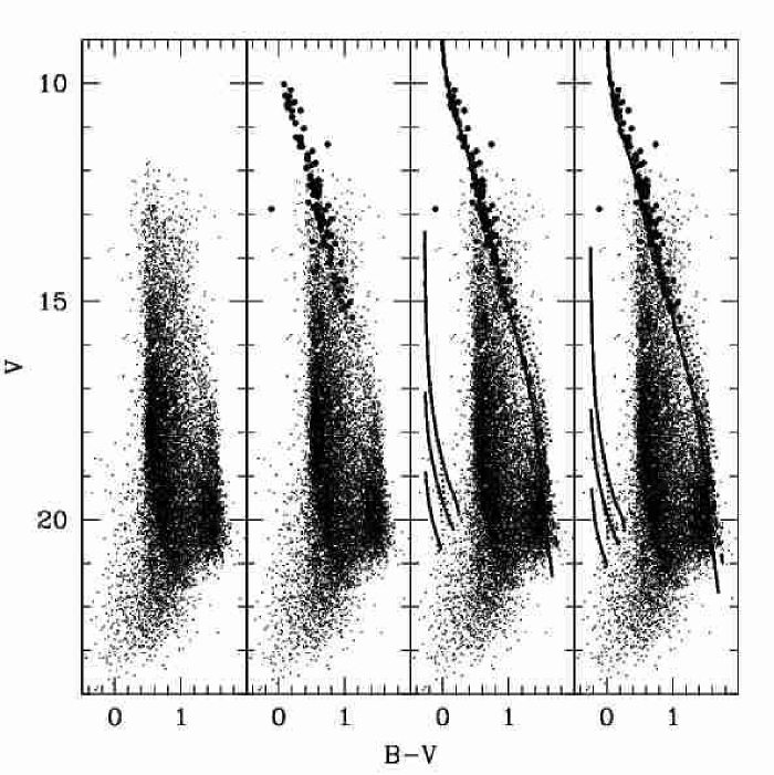
Figure 1.— $\bv,\ V$ color-magnitude diagram for NGC 1039. Left: our photometry alone; note that sources with $V\lesssim 13$ are saturated. Second left: our photometry plus that of cluster members from Jones & Prosser (1996). Second right: combined photometry with isochrones and cooling curves overplotted using the Jones & Prosser (1996) determination of the cluster $(m-M)_{V}$. Right: combined photometry with isochrones and cooling curves adjusted to the cluster $(m-M)_{V}$ derived by Sarajedini et al. (2004). In all panels, small dots indicate our photometry and larger dots show high-probability proper motion cluster members from Jones & Prosser (1996). The main-sequence isochrones are a $Z=0.013$, $\log\tau_{cl}=8.35$ Padova isochrone interpolated from Girardi et al. (2002, solid), a $Z=0.013$, $\log\tau_{cl}=8.35$ Yonsei-Yale isochrone (Demarque et al., 2004, dashed), and the fiducial main sequence of NGC 2168 from von Hippel et al. (2002, dotted) adjusted to the metallicity of NGC 1039. Cooling curves for cluster WDs with cooling times less than 300 Myr and masses of $0.4M_{\odot}$ (top), $0.8M_{\odot}$ (middle) and $1.2M_{\odot}$ (bottom) are shown for DAs (solid) and DBs (dotted).

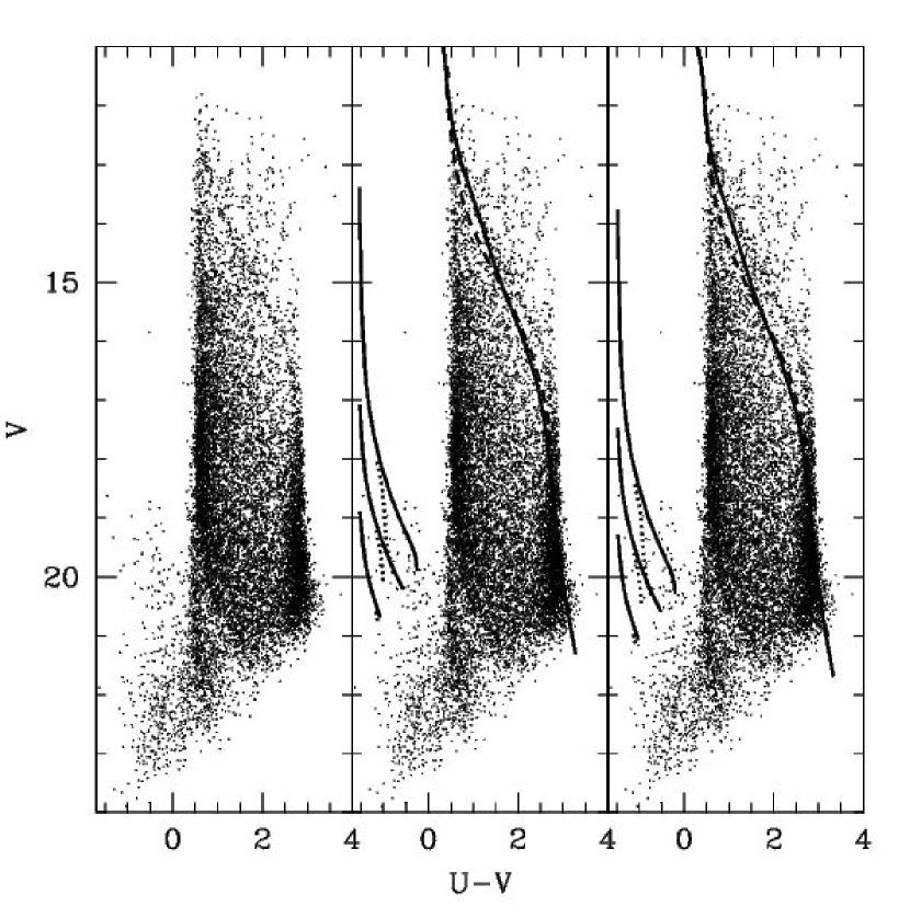
Figure 2.— $U$–$V$, $V$ color-magnitude diagram for NGC 1039. Symbols are as in Figure 1. Left: our photometry alone. Middle: our photometry with isochrones and cooling curves overplotted using the Jones & Prosser (1996) determination of the cluster $(m-M)_{V}$. Right: our photometry with isochrones and cooling curves adjusted to the cluster $(m-M)_{V}$ derived by Sarajedini et al. (2004).

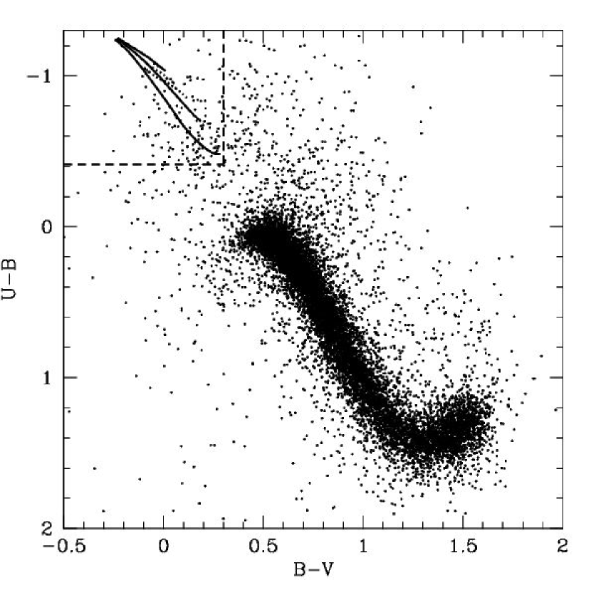
Figure 3.— $\bv,U$–$B$ color-color diagram for NGC 1039. Cooling curves for cluster WDs with cooling times less than 300 Myr and masses of $1.2M_{\odot}$ (top), $0.8M_{\odot}$ (middle), and $0.4M_{\odot}$ (bottom) are shown for DAs (solid) and DBs (dotted). Vertical and horizontal dashed lines mark the boundaries of the WD candidate selection region.

Figure 4.— Lower left-hand regions of the color-magnitude diagrams for NGC 1039. Cooling curves are described in Figures 1 and 2. Dashed lines at the faint ends of the cooling curves mark the colors and $V$ magnitudes of WDs which have been cooling for $\log\tau=8.35$ ($\sim 225$ Myr). Vertical and horizontal dashed lines mark boundaries of the WD candidate selection region. Open circles indicate objects that meet all of our WD selection criteria.

Figure 5.— Upper left-hand region of the color-color diagram for NGC 1039. Cooling curves are described in Figure 3. Vertical and horizontal dashed lines mark boundaries of the WD candidate selection region. Open circles indicate objects that meet all of our WD selection criteria.

Figure 6.— Spectra of WDs in the field of NGC 1039. The spectra of the DB (LAWDS 26) and DC (LAWDS 7) WDs are shown at the top of the left-hand panel, followed by the spectra of the DA WDs in order of decreasing WD $T_{\rm eff}$, from top to bottom and continuing through the right-hand panel.

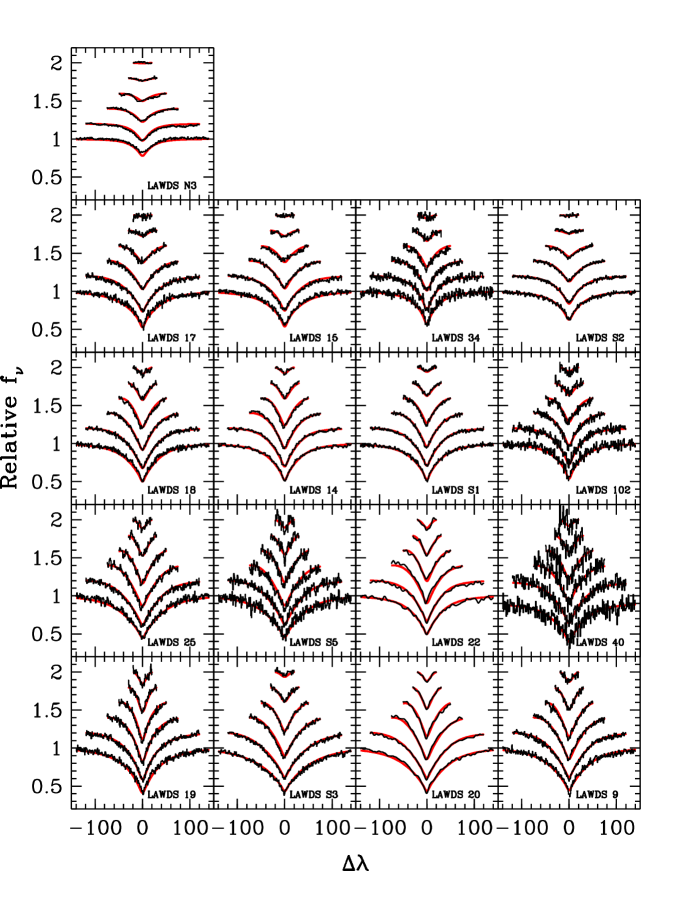
Figure 7.— Balmer-line profiles (light histograms) and best-fit models (heavy curves) for NGC 1039 DA WD spectra. The abscissa shows the offset in Angstroms from the center of each Balmer line. From bottom to top in each panel, the H$\beta$ through H9 line regions are plotted. Each section of spectrum has been normalized to the pseudocontinuum just outside the plotted region and offset arbitrarily in the vertical direction. (A color version of this figure is available in the online journal.)

Figure 8.— Histogram for all spectroscopically confirmed DA WDs in $(m-M)_{V}$ bins of width 0.3 mag. The Jones & Prosser (1996) and Sarajedini et al. (2004) determinations of $(m-M)_{V}$ for NGC 1039 are marked with dashed lines.

Figure 9.— WD candidate selection region of the color-magnitude diagrams for NGC 1039. Cooling curves are described in Figures 1 and 2. The symbols indicate high mass ($>0.8M_{\odot}$) cluster member WDs (large filled circles), lower mass cluster member WDs (intermediate filled circles), the candidate double-degenerate WD (intermediate open circle), the DB (membership undetermined; open triangle), non-cluster member WDs (small filled triangles), non-WDs (crosses), unobserved WD candidates (small open circles), and stars not meeting our selection criteria (small points). Horizontal error bars show $1\sigma$ uncertainties in de-reddened color. $1\sigma$ uncertainties in $M_{V}$ for WDs are smaller than the plotted point sizes.

Figure 10.— WD candidate selection region of the color-color diagram for NGC 1039. Cooling curves are described in Figure 3; symbols are as in Figure 9. Error bars show $1\sigma$ uncertainties in de-reddened color.

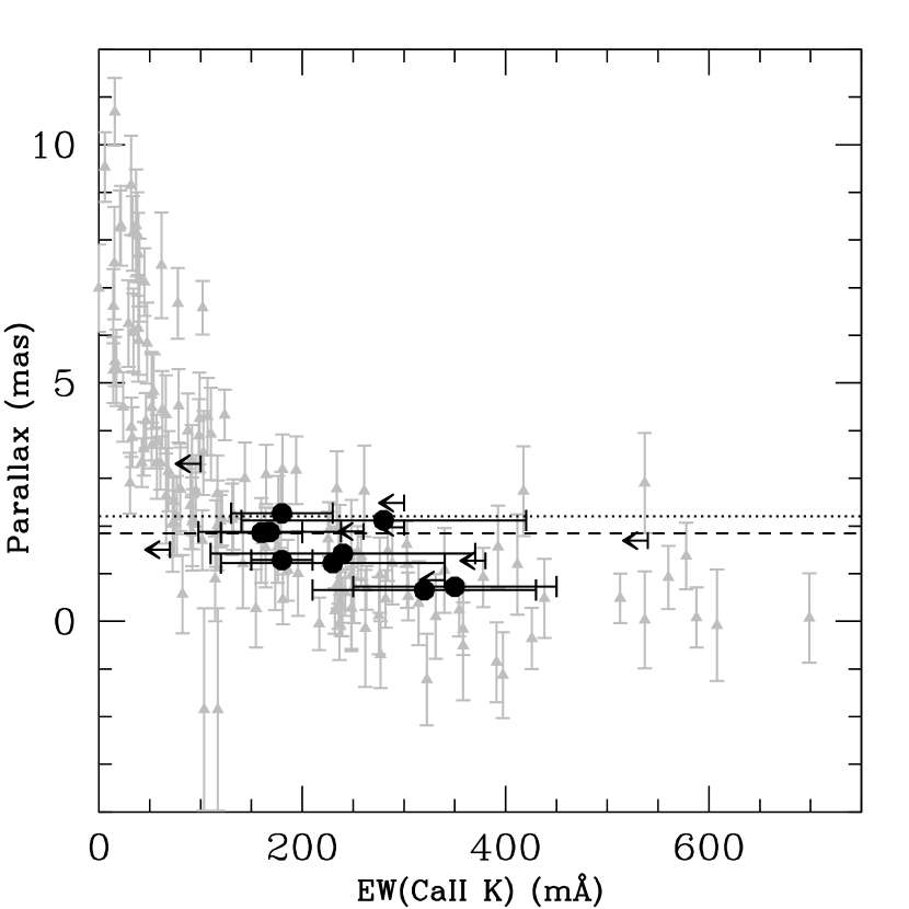
Figure 11.— Measurements presented in Megier et al. (2005, grey triangles) with our Ca II K EWs and parallaxes (computed from our calculated $(m-M)_{0}$ values) overplotted. Our vertical error bars are smaller than the plotted point size. $2\sigma$ EW upper limits on non-detections are also plotted. Our EWs fall within the scatter of the measurements of interstellar Ca II, suggesting that Ca II in the WD spectra is interstellar in origin. Dashed and dotted lines mark the parallax of NGC 1039 as determined by Sarajedini et al. (2004) and Jones & Prosser (1996) respectively.

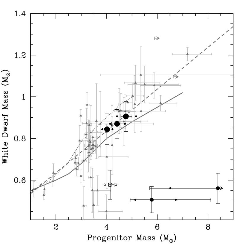
Figure 12.— IFMR with new results over-plotted. Gray triangles show WDs included from the literature. High mass ($>0.8M_{\odot}$) NGC 1039 WDs are represented by large filled circles; low mass NGC 1039 WDs are shown with intermediate-sized filled circles. The open circle represents the candidate double-degenerate binary cluster WD. Error bars on NGC 1039 data points indicate the combined fitting errors for each point. Systematic changes in the location of the NGC 1039 WDs due to the uncertainty in the cluster age are shown by the small points to the left (250 Myr) and right (200 Myr) of each WD. We include the linear IFMR from Ferrario et al. (2005, dashed line), the semi-empirical IFMR of Weidemann (2000, solid curve), and the theoretical, $Z=0.019$ IFMR of Marigo (2001, dotted curve).

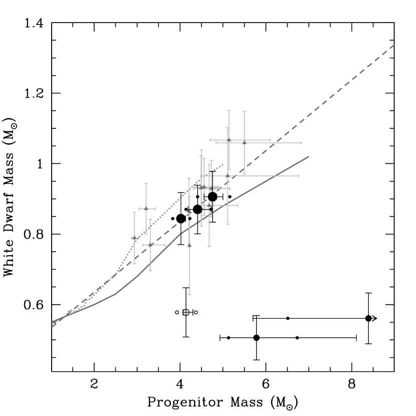
Figure 13.— IFMR with only points from LAWDS plotted; symbols and lines are as in Figure 12. The scatter appears to be smaller here, perhaps indicating that some of the scatter in the combined IFMR is due to the heterogeneity of the data set.

Table 1Transformation equation coefficients.

Instrument	Band	Zero Point	Airmass Term	Color Term	Quadratic Color Term
Nickel	$U$	$A_{0}=21.180\pm 0.091$	$A_{1}=0.419\pm 0.069$	$A_{2}=-0.061\pm 0.002$	$\cdots$
	$B$	$B_{0}=22.752\pm 0.003$	$B_{1}=0.223\pm 0.008$	$B_{2}=-0.083\pm 0.002$	$\cdots$
	$V$	$C_{0}=23.014\pm 0.005$	$C_{1}=0.136\pm 0.005$	$C_{2}=0.060\pm 0.001$	$\cdots$
Mosaic	$U$	$A_{0}=22.942\pm 0.016$	$\cdots$	$A_{2}=-0.167\pm 0.036$	$A_{3}=0.085\tablenotemark{a}$
	$B$	$B_{0}=25.043\pm 0.030$	$\cdots$	$B_{2}=-0.040\pm 0.043$	$\cdots$
	$V$	$C_{0}=24.994\pm 0.043$	$\cdots$	$C_{2}=0.013\pm 0.056$	$\cdots$

Table 2Photometry of candidate WDs in the field of NGC 1039.

LAWDS	R. A.	Decl.	$V$	$\sigma_{V}$	$\bv$	$\sigma_{B-V}$	$U-B$	$\sigma_{U-B}$	Spec. ID	Comments &
ID	(J2000)	(J2000)								References
NGC 1039: LAWDS 4 (catalog )	2:41:19.21	42:47:28.8	19.131	0.032	0.275	0.045	$-$0.650	0.046	QSO	z = 0.784, X-ray source
NGC 1039: LAWDS 7 (catalog )	2:41:06.91	42:42:55.6	19.502	0.032	0.150	0.046	$-$0.509	0.046	DC	$\cdots$
NGC 1039: LAWDS 8 (catalog )	2:41:51.59	42:45:28.3	19.587	0.032	0.079	0.046	$-$0.757	0.046	QSO	z = 1.262, X-ray source
NGC 1039: LAWDS 9 (catalog )	2:40:37.77	42:52:29.6	19.628	0.032	0.119	0.046	$-$0.535	0.046	DA	LB3567 (catalog )
NGC 1039: LAWDS 14 (catalog )	2:41:05.76	42:48:15.3	19.771	0.032	$-$0.029	0.046	$-$0.814	0.046	DA	LB3569 (catalog )
NGC 1039: LAWDS 15 (catalog )	2:40:33.73	42:58:16.7	19.806	0.023	$-$0.027	0.032	$-$1.067	0.032	DA	LB3566 (catalog )
NGC 1039: LAWDS 17 (catalog )	2:40:27.93	42:30:56.6	19.896	0.032	0.078	0.046	$-$1.240	0.046	DA	LB3565 (catalog )
NGC 1039: LAWDS 18 (catalog )	2:40:24.77	42:59:33.1	20.106	0.024	0.105	0.034	$-$0.946	0.033	DA	$\cdots$
NGC 1039: LAWDS 19 (catalog )	2:41:44.93	42:30:05.6	20.130	0.032	0.223	0.046	$-$0.424	0.046	DA	$\cdots$
NGC 1039: LAWDS 20 (catalog )	2:41:09.11	42:43:51.1	20.088	0.032	0.153	0.046	$-$0.445	0.046	DA	LB3570 (catalog )
NGC 1039: LAWDS 22 (catalog )	2:41:39.61	42:43:00.3	20.231	0.033	0.147	0.046	$-$0.545	0.046	DA	LB3575 (catalog )
NGC 1039: LAWDS 23 (catalog )	2:40:51.68	42:58:33.8	20.204	0.023	0.151	0.033	$-$0.836	0.033	QSO	z = 1.949
NGC 1039: LAWDS 25 (catalog )	2:41:55.24	42:53:22.0	20.240	0.023	0.169	0.033	$-$0.500	0.033	DA	LB3576 (catalog )
NGC 1039: LAWDS 26 (catalog )	2:42:00.22	42:59:48.9	20.355	0.023	0.005	0.033	$-$0.899	0.033	DB	A16073 (catalog Cl* NGC 1039 A16073)
NGC 1039: LAWDS 30 (catalog )	2:42:55.48	42:59:00.8	20.760	0.023	0.261	0.034	$-$0.495	0.034	QSO	z = 0.711, A35149 (catalog Cl* NGC 1039 A35149)
NGC 1039: LAWDS 32 (catalog )	2:42:38.40	42:38:46.9	20.776	0.033	0.171	0.047	$-$0.840	0.047	QSO	z = 1.509
NGC 1039: LAWDS 33 (catalog )	2:43:17.19	42:40:52.8	20.820	0.034	0.267	0.049	$-$0.502	0.049	$\cdots$	A43036 (catalog Cl* NGC 1039 A43036)
NGC 1039: LAWDS 34 (catalog )	2:42:59.90	42:38:14.3	20.974	0.034	$-$0.073	0.047	$-$1.024	0.046	DA	$\cdots$
NGC 1039: LAWDS 40 (catalog )	2:40:43.57	42:35:45.6	21.304	0.036	0.056	0.050	$-$0.667	0.049	DA	$\cdots$
NGC 1039: LAWDS 41 (catalog )	2:42:33.98	42:37:13.3	15.846	0.032	0.132	0.045	$-$0.655	0.045	A	A42085 (catalog Cl* NGC 1039 A42085)
NGC 1039: LAWDS 102 (catalog )	2:42:54.29	43:04:00.3	21.156	0.026	$-$0.088	0.036	$-$0.925	0.036	DA	$\cdots$
NGC 1039: LAWDS 103 (catalog )	2:42:58.27	42:53:27.8	21.232	0.026	0.276	0.040	$-$0.533	0.041	$\cdots$	$\cdots$
NGC 1039: LAWDS 104 (catalog )	2:42:54.66	42:40:24.3	21.288	0.036	0.120	0.050	$-$0.590	0.051	$\cdots$	$\cdots$
NGC 1039: LAWDS 105 (catalog )	2:42:29.53	42:38:19.4	21.264	0.035	0.095	0.049	$-$0.506	0.048	$\cdots$	$\cdots$
NGC 1039: LAWDS 107 (catalog )	2:41:42.03	42:38:47.7	21.023	0.034	0.270	0.048	$-$0.517	0.048	$\cdots$	$\cdots$
NGC 1039: LAWDS N3 (catalog )	2:41:11.11	43:13:25.3	18.621	0.032	$-$0.217	0.045	$-$1.238	0.045	DA	$\cdots$
NGC 1039: LAWDS N7 (catalog )	2:42:25.31	43:15:29.7	19.369	0.032	0.199	0.045	$-$0.976	0.045	QSO	z = 2.099
NGC 1039: LAWDS N8 (catalog )	2:42:46.37	43:12:26.4	19.359	0.033	0.205	0.046	$-$0.698	0.046	QSO	z = 1.520
NGC 1039: LAWDS N13 (catalog )	2:40:33.54	43:15:40.5	19.898	0.032	0.119	0.046	$-$0.592	0.046	QSO	z = 1.566
NGC 1039: LAWDS N15 (catalog )	2:41:33.16	43:18:49.3	20.187	0.032	0.145	0.046	$-$0.862	0.046	QSO	z = 1.474
NGC 1039: LAWDS N18 (catalog )	2:40:41.66	43:21:59.6	20.519	0.033	0.196	0.047	$-$0.656	0.047	QSO	z = 1.824
NGC 1039: LAWDS N19 (catalog )	2:41:16.76	43:12:11.3	20.524	0.033	0.173	0.047	$-$0.458	0.048	QSO	z = 1.686
NGC 1039: LAWDS N20 (catalog )	2:43:29.02	43:05:10.4	21.054	0.034	0.072	0.049	$-$0.664	0.049	$\cdots$	$\cdots$
NGC 1039: LAWDS N21 (catalog )	2:42:21.98	43:19:25.1	21.366	0.036	0.135	0.053	$-$0.972	0.052	$\cdots$	$\cdots$
NGC 1039: LAWDS N22 (catalog )	2:41:59.84	43:22:56.4	21.281	0.035	0.031	0.052	$-$1.207	0.051	$\cdots$	$\cdots$
NGC 1039: LAWDS S1 (catalog )	2:41:17.12	42:25:46.8	18.965	0.032	$-$0.044	0.046	$-$0.875	0.046	DA	$\cdots$
NGC 1039: LAWDS S2 (catalog )	2:41:05.05	42:15:59.0	19.330	0.033	$-$0.145	0.046	$-$1.183	0.046	DA	$\cdots$
NGC 1039: LAWDS S3 (catalog )	2:40:59.08	42:15:13.5	19.534	0.033	0.183	0.047	$-$0.546	0.047	DA	$\cdots$
NGC 1039: LAWDS S4 (catalog )	2:41:47.60	42:17:16.5	20.181	0.034	0.166	0.050	$-$0.703	0.049	QSO	z = 1.445
NGC 1039: LAWDS S5 (catalog )	2:41:33.01	42:03:47.3	20.951	0.042	0.028	0.063	$-$0.463	0.060	DA	$\cdots$
NGC 1039: LAWDS S6 (catalog )	2:43:24.85	42:09:34.5	19.914	0.034	0.238	0.049	$-$0.550	0.048	$\cdots$	$\cdots$
NGC 1039: LAWDS S7 (catalog )	2:43:05.14	42:06:24.1	20.495	0.036	0.211	0.053	$-$0.785	0.051	$\cdots$	$\cdots$
NGC 1039: LAWDS S10 (catalog )	2:41:09.14	42:07:48.6	21.327	0.059	$-$0.100	0.086	$-$0.608	0.073	$\cdots$	$\cdots$
NGC 1039: LAWDS S11 (catalog )	2:40:29.04	42:25:51.4	20.858	0.041	0.262	0.069	$-$0.580	0.068	$\cdots$	$\cdots$

Note. — Units of right ascension are hours, minutes and seconds, and units of declination are degrees, arcminutes, and arcseconds. Identifications of “A” indicate non-WD spectra with Balmer-series lines.

Table 3Spectral fits for DA WDs in the field of NGC 1039.

LAWDS	S/N	$T_{\rm eff}$	$\sigma_{T_{\rm eff},{\rm int}}$	$\sigma_{T_{\rm eff},{\rm tot}}$	$\log g$	$\sigma_{\log g,{\rm int}}$	$\sigma_{\log g,{\rm tot}}$	$M_{\mathrm{W}D}$	$\sigma_{M_{\mathrm{W}D}}$	$\tau_{\mathrm{W}D}$	$\sigma_{\tau_{\mathrm{W}D}}$	$M_{V}$	$\sigma_{M_{V}}$	$(m-M)_{V}$	$\sigma_{(m-M)_{V}}$
ID		K	K	K				$M_{\odot}$	$M_{\odot}$	log(yr)	log(yr)
LAWDS 9	115	15300	70	1100	7.82	0.01	0.12	0.506	0.063	8.141	0.132	10.949	0.210	8.679	0.212
LAWDS 14	118	21100	50	1100	7.80	0.02	0.12	0.514	0.059	7.537	0.130	10.348	0.203	9.423	0.206
LAWDS 15	175	25900	50	1100	8.38	0.01	0.12	0.870	0.074	7.791	0.181	10.861	0.231	8.945	0.232
LAWDS 17	189	24700	70	1100	8.44	0.01	0.12	0.906	0.072	7.949	0.158	11.058	0.231	8.838	0.233
LAWDS 18	219	19400	50	1100	7.84	0.01	0.12	0.529	0.065	7.734	0.147	10.559	0.207	9.547	0.208
LAWDS 19	118	11300	50	1100	8.02	0.01	0.12	0.617	0.079	8.652	0.132	11.796	0.313	8.334	0.315
LAWDS 20	110	14700	50	1100	7.92	0.01	0.12	0.561	0.072	8.269	0.135	11.157	0.219	8.931	0.221
LAWDS 22	92	18800	50	1100	7.72	0.01	0.12	0.465	0.055	7.711	0.131	10.444	0.211	9.787	0.214
LAWDS 25	79	15400	50	1100	7.92	0.01	0.12	0.562	0.072	8.201	0.129	11.076	0.204	9.164	0.205
LAWDS 34	70	27700	160	1110	7.76	0.04	0.13	0.512	0.060	7.068	0.064	9.747	0.228	11.227	0.231
LAWDS 40	37	19000	160	1110	7.90	0.04	0.13	0.565	0.078	7.838	0.164	10.683	0.229	10.621	0.232
LAWDS 102	71	24200	100	1100	7.84	0.02	0.12	0.541	0.065	7.300	0.112	10.151	0.212	11.005	0.214
LAWDS N3	239	44000	130	1110	7.74	0.01	0.12	0.558	0.049	6.504	0.050	8.856	0.210	9.765	0.212
LAWDS S1	170	22200	130	1110	7.92	0.02	0.12	0.578	0.070	7.529	0.156	10.432	0.208	8.533	0.210
LAWDS S2	201	31200	100	1100	8.32	0.03	0.12	0.844	0.074	7.287	0.215	10.368	0.223	8.962	0.225
LAWDS S3	170	14700	100	1100	8.36	0.03	0.12	0.842	0.073	8.570	0.123	11.818	0.231	7.716	0.233
LAWDS S5	67	15900	200	1120	7.96	0.03	0.12	0.587	0.072	8.182	0.132	11.077	0.204	9.874	0.208

Table 4Progenitor masses for NGC 1039 WDs.

LAWDS	$M_{\mathrm{W}D}$	$\sigma_{M_{\mathrm{W}D}}$	$M_{init}\,(M_{\odot})$
ID	$M_{\odot}$	$M_{\odot}$	$\log\tau_{cl}=8.30$	$\log\tau_{cl}=8.35$	$\log\tau_{cl}=8.40$
LAWDS 9	0.506	0.063	6.73	$5.78^{+2.33}_{-0.85}$	5.13
LAWDS 15	0.870	0.074	4.72	$4.41^{+0.32}_{-0.22}$	4.14
LAWDS 17	0.906	0.072	5.16	$4.76^{+0.24}_{-0.20}$	4.41
LAWDS 20	0.561	0.072	18.38	$8.39^{+9.99}_{-2.69}$	6.51
LAWDS S1	0.578	0.070	4.37	$4.14^{+0.16}_{-0.07}$	3.93
LAWDS S2	0.844	0.074	4.23	$4.02^{+0.11}_{-0.06}$	3.83

Table 5Ca II K EW measurements for WDs in the field of NGC 1039.

LAWDS	Ca II K EW	dEW
ID	mÅ	mÅ
LAWDS 7	$<147$	$\cdots$
LAWDS 9	280	140
LAWDS 14	$<70$	$\cdots$
LAWDS 15	168	70
LAWDS 17	$<300$	$\cdots$
LAWDS 18	240	130
LAWDS 19	$<300$	$\cdots$
LAWDS 20	$<260$	$\cdots$
LAWDS 22	$<380$	$\cdots$
LAWDS 25	$<540$	$\cdots$
LAWDS 26	230	100
LAWDS 34	320	110
LAWDS 40	$<340$	$\cdots$
LAWDS 102	350	100
LAWDS N3	180	30
LAWDS S1	180	50
LAWDS S2	160	40
LAWDS S3	$<100$	$\cdots$
LAWDS S5	230	110

Table 6Comparison of WD model colors with observed colors.

LAWDS	$(m-M)_{V}$	$(B-V)$	$(B-V)_{0}$	$E(B-V)$	$(U-V)$	$(U-V)_{0}$	$E(U-V)$
LAWDS 9	8.679	0.119	0.054	0.065	-0.416	-0.648	0.232
LAWDS 15	8.945	-0.027	-0.128	0.101	-1.094	-1.210	0.116
LAWDS 17	8.838	0.078	-0.108	0.186	-1.162	-1.167	0.005
LAWDS 20	8.931	0.153	0.084	0.069	-0.292	-0.603	0.311
LAWDS S1	8.533	-0.044	-0.092	0.048	-0.919	-1.061	0.142
LAWDS S2	8.962	-0.145	-0.201	0.056	-1.328	-1.374	0.046

References

- Anthony-Twarog (1982) Anthony-Twarog, B. J. 1982, ApJ, 255, 245
- Asplund et al. (2004) Asplund, M., Grevesse, N., Sauval, A. J., Allende Prieto, C., & Kiselman, D. 2004, A&A, 417, 751
- Bergeron et al. (1990) Bergeron, P., Liebert, J., & Greenstein, J. L. 1990, ApJ, 361, 190
- Bergeron et al. (1992) Bergeron, P., Saffer, R. A., & Liebert, J. 1992, ApJ, 394, 228
- Bergeron et al. (1995) Bergeron, P., Wesemael, F., & Beauchamp, A. 1995, PASP, 107, 1047
- Bertelli et al. (1994) Bertelli, G., Bressan, A., Chiosi, C., Fagotto, F., & Nasi, E. 1994, A&AS, 106, 275
- Claver et al. (2001) Claver, C. F., Liebert, J., Bergeron, P., & Koester, D. 2001, ApJ, 563, 987
- Cohen et al. (1994) Cohen, J. G., Cromer, J., & Southard, S., Jr. 1994, in ASP Conf. Proc. 61, Astronomical Data Analysis Software and Systems III (San Francisco, CA: ASP), 469
- Dekel & Silk (1986) Dekel, A. & Silk, J. 1986, ApJ, 303, 39
- Demarque et al. (2004) Demarque, P., Woo, J.-H., Kim, Y.-C., & Yi, S. K. 2004, ApJS, 155, 667
- Ferrario et al. (2005) Ferrario, L., Wickramasinghe, D., Liebert, J., & Williams, K. A. 2005, MNRAS, 361, 1131
- Finkbeiner (2003) Finkbeiner, D. P. 2003, ApJS, 146, 407
- Fontaine et al. (2001) Fontaine, G., Brassard, P., & Bergeron, P. 2001, PASP, 113, 409
- Fontaine & Wesemael (1987) Fontaine, G., & Wesemael, F. 1987, in Proc. IAU Colloq. 95, Second Conference on Faint Blue Stars, (Cambridge: Cambridge Univ. Press), 319
- Girardi et al. (2002) Girardi, L., Bertelli, G., Bressan, A., Chiosi, C., Groenewegen, M. A. T., Marigo, P., Salasnich, B., & Weiss, A. 2002, A&A, 391, 195
- Girardi et al. (2000) Girardi, L., Bressan, A., Bertelli, G., & Chiosi, C. 2000, A&AS, 141, 371
- Green (1980) Green, R. F. 1980, ApJ, 238, 685
- Hansen et al. (2002) Hansen, B. M. S., et al. 2002, ApJ, 574, L155
- Hansen et al. (2004) Hansen, B. M. S., et al. 2004, ApJS, 155, 551
- Hansen et al. (2007) Hansen, B. M. S., et al. 2007, ApJ, 671, 380
- Harris et al. (2006) Harris, H. C., et al. 2006, AJ, 131, 571
- Holberg & Bergeron (2006) Holberg, J. B., & Bergeron, P. 2006, AJ, 132, 1221
- Ianna & Schlemmer (1993) Ianna, P. A., & Schlemmer, D. M. 1993, AJ, 105, 209
- Jones & Prosser (1996) Jones, B. F. & Prosser, C. F. 1996, AJ, 111, 1193
- Kalirai et al. (2007) Kalirai, J. S., Bergeron, P., Hansen, B. M. S., Kelson, D. D., Reitzel, D. B., Rich, R. M., & Richer, H. B. 2007, ApJ, 671, 748
- Kalirai et al. (2008) Kalirai, J. S., Hansen, B. M. S., Kelson, D. D., Reitzel, D. B., Rich, R. M., & Richer, H. B. 2008, ApJ, 676, 594
- Kalirai et al. (2005) Kalirai, J. S., Richer, H. B., Reitzel, D., Hansen, B. M. S., Rich, R. M., Fahlman, G. G., Gibson, B. K., & von Hippel, T. 2005, ApJ, 618, L123
- Kilic et al. (2007) Kilic, M., Allende Prieto, C., Brown, W. R., & Koester, D. 2007, ApJ, 660, 1451
- Koester (1980) Koester, D. 1980, A&AS, 39, 401
- Koester & Reimers (1981) Koester, D., & Reimers, D. 1981, A&A, 99, L8
- Koester & Reimers (1996) Koester, D., & Reimers, D. 1996, A&A, 313, 810
- Koester et al. (1979) Koester, D., Schulz, H., & Weidemann, V. 1979, A&A, 76, 262
- Koester et al. (2001) Koester, D., et al. 2001, A&A, 378, 556
- Landolt (1992) Landolt, A. U. 1992, AJ, 104, 340
- Liebert et al. (2005) Liebert, J., Bergeron, P., & Holberg, J. B. 2005, ApJS, 156, 47
- Luyten (1961) Luyten, W. J. 1961, The Observatory, Univ. Minnesota, Minneapolis, 1953, 23, 1
- Marigo (2001) Marigo, P. 2001, A&A, 370, 194
- Massey et al. (2006) Massey, P., Olsen, K. A. G., Hodge, P. W., Strong, S. B., Jacoby, G. H., Schlingman, W., & Smith, R. C. 2006, AJ, 131, 2478
- Megier et al. (2005) Megier, A., Strobel, A., Bondar, A., Musaev, F. A., Han, I., KreŁowski, J., & Galazutdinov, G. A. 2005, ApJ, 634, 451
- Meynet et al. (1993) Meynet, G., Mermilliod, J.-C., & Maeder, A. 1993, A&AS, 98, 477
- Oke et al. (1995) Oke, J. B., et al. 1995, PASP, 107, 375
- Pinsonneault et al. (1998) Pinsonneault, M. H., Stauffer, J., Soderblom, D. R., King, J. R., & Hanson, R. B. 1998, ApJ, 504, 170
- Poelarends et al. (2008) Poelarends, A. J. T., Herwig, F., Langer, N., & Heger, A. 2008, ApJ, 675, 614
- Raffauf et al. (2001) Raffauf, E., Bavender, M. J., Steinhauer, A., Deliyannis, C. P., Sarajedini, A., Bailyn, C., & Platais, I. 2001, BAAS, 33, 843
- Rieke & Lebofsky (1985) Rieke, G. H., & Lebofsky, M. J. 1985, ApJ, 288, 618
- Romanishin & Angel (1980) Romanishin, W. & Angel, J. R. P. 1980, ApJ, 235, 992
- Sarajedini et al. (2004) Sarajedini, A., Brandt, K., Grocholski, A. J., & Tiede, G. P. 2004, AJ, 127, 991
- Schuler et al. (2003) Schuler, S. C., King, J. R., Fischer, D. A., Soderblom, D. R., & Jones, B. F. 2003, AJ, 125, 2085
- Simon (2000) Simon, T. 2000, PASP, 112, 599
- Sion & Liebert (1977) Sion, E. M., & Liebert, J. 1977, ApJ, 213, 468
- Stetson (1987) Stetson, P. B. 1987, PASP, 99, 191
- Stetson (1990) Stetson, P. B. 1990, PASP, 102, 932
- Vanden Berk et al. (2001) Vanden Berk, D. E., et al. 2001, AJ, 122, 549
- van Dokkum (2001) van Dokkum, P. G. 2001, PASP, 113, 1420
- von Hippel et al. (2002) von Hippel, T., Steinhauer, A., Sarajedini, A., & Deliyannis, C. P. 2002, AJ, 124, 1555
- von Hippel et al. (2005a) von Hippel, T., Winget, D. E., Jefferys, W. H., & Scott, J. G. 2005a, in ASP Conf. Ser. 334, 14th European Workshop on White Dwarfs, ed. D. Koester & S. Moehler (San Francisco, CA: ASP), 77
- von Hippel et al. (2005b) von Hippel, T., et al. 2005b, in ASP Conf. Ser. 334, 14th European Workshop on White Dwarfs, ed. D. Koester & S. Moehler (San Francisco, CA: ASP), 3
- Weidemann (1977) Weidemann, V. 1977, A&A, 59, 411
- Weidemann (2000) Weidemann, V. 2000, A&A, 363, 647
- Wesemael et al. (1994) Wesemael, F., et al. 1994, ApJ, 429, 369
- Williams (2004) Williams, K. A. 2004, ApJ, 601, 1067
- Williams (2007) Williams, K. A. 2007, Astron. Soc. Pac. Conf. Series, 372, 85
- Williams & Bolte (2007) Williams, K. A. & Bolte, M. 2007, AJ, 133, 1490
- Williams et al. (2004a) Williams, K. A., Bolte, M., & Koester, D. 2004a, ApJ, 615, L49
- Williams et al. (2004b) Williams, K. A., Bolte, M., & Liebert, J. W. 2004b, AJ, 128, 1784
- Williams et al. (2008) Williams, K. A., Bolte, M., & Koester, D. 2008, ApJ, submitted
- Winget et al. (1987) Winget, D. E., Hansen, C. J., Liebert, J., van Horn, H. M., Fontaine, G., Nather, R. E., Kepler, S. O., & Lamb, D. Q. 1987, ApJ, 315, L77
- Wood (1995) Wood, M. A. 1995, White Dwarfs (Lecture Notes in Physics), Vol. 443, (Berlin:Springer), 41
- Yi et al. (2001) Yi, S., Demarque, P., Kim, Y.-C., Lee, Y.-W., Ree, C. H., Lejeune, T., & Barnes, S. 2001, ApJS, 136, 417
- Zuckerman et al. (2003) Zuckerman, B., Koester, D., Reid, I. N., Hünsch, M. 2003, ApJ, 596, 477