Characterization of turbulence in inhomogeneous anisotropic flows

Abstract

We introduce a global quantity $\delta$ that characterizes turbulent fluctuations in inhomogeneous anisotropic flows. This time-dependent quantity is based on spatial averages of global velocity fields rather than classical temporal averages of local velocities. $\delta(t)$ provides a useful quantitative characterization of any turbulent flow through generally only two parameters, its time average $\bar{\delta}$ and its variance $\delta_{2}$. Properties of $\bar{\delta}$ and $\delta_{2}$ are experimentally studied in the typical case of the von Kármán flow and used to characterize the scale by scale energy budget as a function of the forcing mode as well as the transition between two flow topologies.

I Introduction

The classical theory of homogeneous isotropic turbulence applies to flows with zero velocity average so that all the turbulence properties are contained in the temporal velocity fluctuations Frisch . Real turbulent flows, with non trivial boundary conditions and external forcing, often possess a non-zero mean flow that may or may not be stationary . Quantifying the influence of turbulent fluctuations on the flow dynamics has been the corner stone of turbulence theory. In early experimental works, velocity measurements were performed through hot wire probes providing temporal variations of the velocity at fixed points. A natural parameter quantifying the intensity of turbulence has therefore been introduced as:

$$i=\sqrt{\frac{\overline{V^{2}}-\overline{V}^{2}}{\overline{V}^{2}}},$$

where $V$ is the velocity and $\overline{X}$ refers to the time average of variable $X$. While such a parameter clearly characterizes fluctuations in a homogeneous flow, one may question its relevance in more general anisotropic inhomogeneous flows where turbulence intensity depends on the measurement point (cf. Figs. 1(a) and (d)). For example, $i$ diverges around stagnation points or shears so that no robust global quantity can be built by integrating or averaging $i$ over the whole flow. This question is receiving an increasing interest since the advent of Particle Image Velocimetry (PIV) measurements which provide instantaneous snapshots of the velocity field.

(a)	(b)	(c)
\psfrag{r/R}[c][1]{$r/R$}\psfrag{z/Z}[c][1.1]{$z/Z$}\includegraphics[width=166.94461pt]{figure1a.eps}	\psfrag{r/R}[c][1]{$r/R$}\psfrag{z/Z}[c][1.1]{$z/Z$}\includegraphics[width=130.08731pt]{figure1b.eps}	\psfrag{r/R}[c][1]{$r/R$}\psfrag{z/Z}[c][1.1]{$z/Z$}\includegraphics[width=130.08731pt]{figure1c.eps}
(d)	(e)	(f)
\psfrag{r/R}[c][1]{$r/R$}\psfrag{z/Z}[c][1.1]{$z/Z$}\includegraphics[width=166.94461pt]{figure1d.eps}	\psfrag{r/R}[c][1]{$r/R$}\psfrag{z/Z}[c][1.1]{$z/Z$}\includegraphics[width=130.08731pt]{figure1e.eps}	\psfrag{r/R}[c][1]{$r/R$}\psfrag{z/Z}[c][1.1]{$z/Z$}\includegraphics[width=130.08731pt]{figure1e.eps}

Figure 1: Maps of turbulence intensity $i$, (a) and (d), corresponding time averaged, (b) and (e), and typical instantaneous, (c) and (f), velocity fields for two von Kármán flows ((a-c) and (d-f)) at the same Reynolds number but with slightly different geometry. Both flows correspond to the same experimental setup —TM60$(+)$—, except for a narrow annulus inserted in the median plane of the flow in (d-f). In (a) and (d), for better visibility, the gray scale has been saturated at $i=6$ since values up to $i\sim$ 10⁴ can be reached in the median plane due to weak mean velocities and large fluctuations. Additionally, vectors of the instantaneous velocities have been scaled by half with respect to the mean field vectors.

An illustration of the importance of that issue may be given in the typical inhomogeneous anisotropic case of the von Kármán flow. This flow, generated in between two counter-rotating co-axial impellers, has received a lot of interest cadot95 ; labbe96a ; mordant97a ; ravelet2004 ; nore05 as a simple way to obtain experimentally a very large Reynolds number flow in a compact design ($Re\sim 10^{6}$ in a table top water apparatus). In the equatorial shear layer of such a flow, fluctuations are large and exhibit similar local properties as in large Reynolds number experimental facilities devoted to homogeneous turbulence Maurer1994 ; Tabeling1996 ; labbe96a ; Arneodo1996 . Away from the shear layer, one observes a decrease of the turbulence intensity theselouis ; marie04 as seen in Figs. 1(a) and (d). Overall, the flow is strongly turbulent, so that the instantaneous velocity fields, measured by means of a PIV system, strongly differ in a non-trivial manner from their time average (cf. Figs. 1(b) and (c)).

First, we introduce in Sec. II a global time-dependent quantity $\delta(t)$ that allows to characterize globally turbulent fluctuations in any inhomogeneous anisotropic flow. In Sec. III, we present our experimental setup and show how to compute practically $\delta(t)$ from Stereoscopic Particule Image Velocimetry (SPIV) measurements. In Sec. IV, we first show that $\delta(t)$ provides a useful quantitative characterization of turbulent flows through generally only two parameters, its time average $\bar{\delta}$ and its variance $\delta_{2}$, that quantify respectively the level of fluctuations compared to the mean flow and their ability to disturb the mean flow. These two quantities are introduced as a generalization of the classical local turbulence intensity $i$. Finally, we discuss applications of these new global measures of turbulence intensity: we show how these parameters may be used to study the influence of the forcing conditions on the flow.

II Generalization of the turbulence intensity

We consider a general anisotropic inhomogeneous turbulent flow, with velocity field $V(\vec{x},t)=[u(\vec{x},t),v(\vec{x},t),w(\vec{x},t)]$. In order to smooth out the possible spatial inhomogeneities of the turbulence intensity, we define a scalar quantity through :

$$\delta(t)=\frac{\langle V^{2}(t)\rangle}{\langle\overline{V}^{2}\rangle},$$

where $\langle X\rangle$ and $\overline{X}$ refer respectively to spatial and time average of $X$, and $V(\vec{x},t)^{2}=u^{2}+v^{2}+w^{2}$ is the local kinetic energy density at time $t$. The quantity $\delta$ can also be viewed as the ratio of the total kinetic energy of the instantaneous flow to the total kinetic energy of the mean flow:

$$\delta(t)=\frac{E\left(V(t)\right)}{E\left(\overline{V}\right)}.$$ (1)

Note that this scalar parameter is time dependent and generally widely fluctuates in time (cf. Fig. 2). We then define two time independent parameters, $\bar{\delta}$ and $\delta_{2}$, that are respectively the time average and the variance of $\delta(t)$ as:

$$\bar{\delta}=\overline{\langle V^{2}(t)\rangle}/{\langle\overline{V}^{2}\rangle},$$

$$\delta_{2}=\sqrt{\overline{\delta(t)^{2}}-\overline{\delta(t)}^{2}}.$$

We show in Sec. III that these two quantities fully characterize $\delta(t)$ provided that the considered time series of sampled fields are uncorrelated. Two interesting physical interpretations of $\bar{\delta}$ can be drawn: first, in a homogeneous turbulent flow, $\bar{\delta}=i^{2}+1$, so that $\bar{\delta}$ is a global generalization of the local turbulence intensity; second, for real flows such as the von Kármán flow, $\bar{\delta}$ contains an additional information regarding how far the instantaneous flow is from the mean flow. Indeed,

$$\left(\bar{\delta}-1\right)\langle\overline{V}^{2}\rangle = \overline{\langle(V-\overline{V})^{2}\rangle}$$

$$= \frac{1}{\cal{V}}\overline{\int_{\cal{V}}d^{3}\vec{x}\left(V-\overline{V}\right)^{2}},$$

where the sum runs over the volume $\cal{V}$ of the flow. The quantity under the overline is nothing but the square of the mean distance (using norm 2) between the instantaneous flow and the mean flow in the functional space. Therefore, the quantity $\bar{\delta}-1$ measures how far, on average, the instantaneous velocity field is from its time average. If $\bar{\delta}$ is close to one, one therefore expects the instantaneous flow to strongly resemble the mean flow. If $\bar{\delta}$ is much greater than $1$, the instantaneous field will be more remote from the mean flow. This interpretation of $\delta$ will be used in appendix A to draw a rough study of the convergence of the von Kármán flow toward its time average.

\psfrag{d}[c][1.2]{$\delta$}\includegraphics[width=216.81pt]{figure2.eps}

Figure 2: Example of the temporal evolution of $\delta(t)$ at two time scales: a full record of about 20 minutes on the left, and a focus on a 40 seconds sample on the right. A schematic illustration of the meaning of $\bar{\delta}$ and $\delta_{2}$ is also provided over the longest time record.

III Experimental setup and data processing

III.1 The von Kármán flow

III.1.1 Experimental setup

In order to illustrate and apply these concepts, we have worked with a specific axisymmetric turbulent flow: the von Kármán flow generated by two counter-rotating impellers in a cylindrical vessel. The cylinder radius and height are respectively $R=100$ mm and $240$ mm. We have used two sets of impellers named TM60 and TM73 . These two models are flat disks of respective diameter $185$ and $150$ mm fitted with radial blades of height $20$ mm and respective curvature radius $50$ and $92.5$ mm. The inner faces of the discs are $H=180$ mm apart.
Impellers are driven by two independent motors rotating up to typically $10$ Hz. More details about the experimental setup can be found in ravelet2005 . The motor frequencies can be either set equal to get exact counter-rotating regime, or set to different values $f_{1}\neq f_{2}$. We define two forcing conditions associated with the concave (resp. convex) face of the blades going forward, denoted in the sequel by sense $(-)$ (resp. $(+)$ ). We also work with two different vessel geometries, allowing the optional insertion of an annulus —thickness $5$ mm, inner diameter $170$ mm— in the equatorial plane. Both the forcing condition and the annulus insertion strongly influence the level of fluctuation in the flow, thereby allowing to test experimentally the sensitivity and the relevance of $\delta(t)$, $\bar{\delta}$ and $\delta_{2}$. The working fluid is water.

III.1.2 Control parameters

From the two motor frequencies, $f_{1}$ and $f_{2}$, we define two control parameters: a Reynolds number, $Re$, and a rotation number, $\theta$. For the experiments described in this paper, the Reynolds number,

$$Re=\pi(f_{1}+f_{2})R^{2}\nu^{-1},$$

where $\nu$ is the fluid kinematic viscosity, ranges from $1.25\times 10^{5}$ to $5\times 10^{5}$ so that the turbulence can be considered fully developed. The rotation number,

$$\theta=\frac{f_{1}-f_{2}}{f_{1}+f_{2}},$$

measures the relative influence of global rotation over a typical turbulent shear frequency. Indeed, the exact counter-rotating regime corresponds to $\theta=0$ and, for a non-zero rotation number, our experimental system is similar, within lateral boundaries, to an exact counter-rotating experiment at frequency $f=(f_{1}+f_{2})/2$, with an overall global rotation at frequency $(f_{1}-f_{2})/2$ theselouis ; ravelet2004 . In our experiments, we vary $\theta$ from $-1$ to $+1$, exploring a regime of relatively weak rotation to shear ratio.

III.1.3 Mean flow topology

In the exact counter-rotating regime, i.e. for $\theta=0$, the standard mean flow is divided into two toric recirculation cells separated by an azimuthal shear layer (cf. Fig. 1(b) and (e)). As $\theta$ is driven away from zero, a change of topology occurs at a critical value $\theta_{c}$: the mean flow bifurcates from the two counter-rotating recirculation cells to a single cell ravelet2004 . $\theta_{c}$ depends on the forcing and the geometry. For example, in the configuration with TM73 impellers, rotation sense $(+)$ and the annulus, we measure $\theta_{c}=0.17\pm 0.01$ through torque measurements. In the case TM60$(-)$, this turbulent bifurcation becomes highly singular and gives rise to multistability between the two turbulent flow symmetries, $O(2)$/$SO(2)$ ravelet2004 .

III.2 Measurements and data processing

Measurements are done with a Stereoscopic Particle Image Velocimetry (SPIV) system. The SPIV data provide the radial, axial and azimuthal velocity components on a 95$\times$66 points grid covering a whole meridian plane of the flow through a time series of about 5000 regularly sampled values. The sampling frequency is set between 1 and 4 Hz, corresponding to one sample record every 1 to 10 impeller rotations. The total acquisition time is about ten minutes, i.e. one order of magnitude longer than the characteristic time of the slowest patterns of the turbulent flow. Fast scales are statistically sampled.
The velocity fields are non-dimensionalized using a typical velocity $V_{0}=2\pi R(f_{1}+f_{2})/2$ based on the radius of the cylinder and the rotation frequencies of the impellers. The resulting velocity fields are windowed so as to fit to the boundaries of the flow and remove spurious velocities measured in the impellers and the boundaries. The resulting fields consist of 58$\times$58 points velocity maps. Two types of filtering are further applied to clean the data: first, a global filter to get rid of all velocities larger than $3\times V_{0}$; then, a local filter (based on velocities of nearest neighbours) to remove isolated spurious vectors. Typically, 1 $\%$ of the data are changed by this processing.

III.3 Data analysis

We use two different methods to compute $\delta(t)$ from our PIV measurements. In the direct method, we compute $\delta$ by spatially averaging the kinetic energy density of instantaneous and time averaged flows. Since we measure the full velocity field in a single meridian plane only, we compute 3D spatial averages of any quantity $X$ assuming the statistical axisymmetry of the von Kármán flow such as:

$$\langle X(r,z)\rangle=\frac{1}{R^{2}H}\int^{R}_{-R}|r|dr\int^{H/2}_{-H/2}dz\,X(r,z).$$

Since velocity fields are discrete in space and time, spatial integration is done with a classical numerical trapezoid summation method whereas time integration is performed through simple summation. The parameter $\delta$ can also be obtained by a spectral method. For this, we compute the spatial Power Spectral Density (PSD) of the discrete velocity fields as:

$$\widetilde{E}(k_{r},k_{z},t)=\widetilde{W}\,\widetilde{W}^{*},$$

where $\widetilde{W}=\widetilde{W}(k_{r},k_{z},t)$ is the two dimensional spatial Fourier transform of $W(r,z,t)=\sqrt{|r|}\,V(r,z,t)$ and $\widetilde{W}^{*}$ its complex conjugate. Then, we compute $\delta$ using Parseval’s identity:

$$\int\int|r|drdz\,V^{2}=\int\int dk_{r}dk_{z}\widetilde{W}\widetilde{W}^{*},$$

and get:

$$\delta(t)=\frac{\int\int dk_{r}dk_{z}\widetilde{E}(k,t)}{\int\int dk_{r}dk_{z}\,\widetilde{E}_{0}(k)},$$ (2)

where $\widetilde{E}_{0}$ is the PSD of the time averaged flow

$$\widetilde{E}_{0}(k_{r},k_{z},t)=\widetilde{\overline{W}}\,\widetilde{\overline{W}}^{*}.$$

IV Results and applications

IV.1 Basic properties of $\delta$

IV.1.1 Statistical properties

As discussed in Sec. II, $\delta(t)$ widely fluctuates in time. However, its statistical properties in the exact counter-rotating case are rather simple since its probability density function (PDF) is nearly Gaussian as illustrated in Fig. 3(a). Actually, this property holds at different Reynolds numbers (cf. Fig. 3(a)) and for all forcing and geometry conditions studied in the present paper (cf. Fig. 3(b)). A striking feature is that global rotation does not change the statistical properties of the flow since the PDFs are Gaussian at any $\theta$. Consequently, we can describe and fully characterize the total energy temporal distribution using only the two scalar parameters $\bar{\delta}$ and $\delta_{2}$.

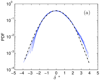
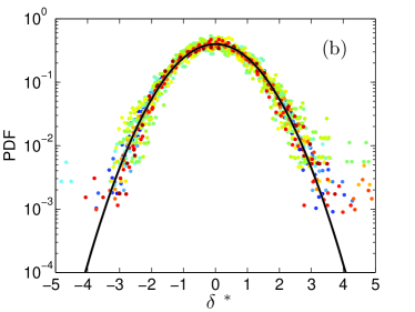
Figure 3: Centered and reduced Probability Density Function of $\delta(t)$, (a) for the TM73$(-)$ configuration with annulus at seven different Reynolds numbers ranging from $1.25\times 10^{5}$ to $5\times 10^{5}$, and (b) for the TM73$(+)$ configuration without annulus for $16$ experiments performed with different values of rotation number $\theta=(f_{1}-f_{2})/(f_{1}+f_{2})$ ranging from $0$ to $1$. $\delta^{*}=(\delta-\bar{\delta})/\delta_{2}$ is the centered reduced value of $\delta$. The dash-dotted lines are Gaussian functions of zero mean and unit variance.

IV.1.2 Dependence on the Reynolds number

For a given forcing, we observe a very weak dependence of $\bar{\delta}$ with $Re$ in the studied range as one can see in Fig. 4. The largest dispersions, of the order of $8\%$, are observed in the negative rotation sense for both TM60 and TM73 impellers without annulus. For any other forcing condition, the dispersion is less than $5\%$. Similar conclusions hold for $\delta_{2}$ represented in Fig. 4 using error bars. This behavior is not surprising since in our water experiments the Reynolds number is so large that we are in the fully developed turbulent regime where statistical properties have already been shown not to depend on the Reynolds number monchaux2006 ; ravelet2008 ; monchaux07c . On the contrary, we expect a different behavior when lowering the Reynolds number monchaux2006 , since, in the limit of very low $Re$, the instantaneous flow is laminar and identical to the mean flow: $\delta(t)=\bar{\delta}=1$. The study of the transition between laminar and fully turbulent regime requires the use of glycerol-water mixing and is beyond the scope of the present paper. Note however that this transition has already been studied in the von Kármán experiment —TM60$(-)$ without annulus— by Ravelet et al. ravelet2008 using a one point measurement Laser Doppler Velocimetry system. It has been shown that the local value of the variance of the azimuthal velocity, $\overline{v_{\theta}^{2}}-\overline{v}_{\theta}^{2}$, behaves as $(Re-Re_{c})^{1/2}$ and saturates above $Re_{t}=3300$, where $Re_{c}=330$ corresponds to the transition from steady to oscillatory laminar flow and $Re_{t}$ to the onset of the fully turbulent inertial regime. A similar behaviour is encountered in Direct Numerical Simulations of the Taylor-Green flow LavalDyn where an increase of $\bar{\delta}$ from 1 at low $Re$ to a saturation value of 3 for $Re$ above $10^{3}$ has been observed.

\psfrag{d}[c][1.2]{$\bar{\delta}$}\includegraphics[width=216.81pt]{figure4.eps}

Figure 4: $\bar{\delta}$ as a function of Reynolds number $Re$. Negative $Re$ correspond to rotation sense $(-)$. (a) and (b) correspond respectively to TM73 and TM60 impellers, with ($\circ$), and without ($\scriptstyle\square$) annulus. Dash-dotted lines corresponds to the mean value of $\bar{\delta}$ for each configuration and $\delta_{2}$ is represented using error bars.

IV.2 Influence of forcing and annulus

It is difficult to estimate turbulence intensity by simply looking at an instantaneous velocity field (cf. Figs. 1(c) and (f)). To achieve this, the local turbulence intensity $i$ maps (cf. Figs. 1(a) and (d)) constitutes a good qualitative tool to estimate the overall turbulence intensity and structure of the considered flow. However, a quantity like $\delta$ is needed to provide a global quantitative tool.

IV.2.1 Effect of impeller and vessel geometry

As reported in Table 1, the values of $\bar{\delta}$ and $\delta_{2}$ allow to quantify the differences in the turbulence fluctuations level as a function of the forcing configurations (TM60 and TM73, with or without annulus).

	$\bar{\delta}$				$\delta_{2}$
Impellers	TM60		TM73		TM60		TM73
Sense	$(-)$	$(+)$	$(-)$	$(+)$	$(-)$	$(+)$	$(-)$	$(+)$
Without annulus	2.64	2.18	2.22	2.02	0.30	0.24	0.24	0.18
With annulus	1.52	1.47	1.50	1.48	0.11	0.15	0.11	0.12

Table 1: Values of $\bar{\delta}$ and $\delta_{2}$ for various configurations.

The major result of Table 1 is the effect of the annulus which systematically reduces $\bar{\delta}$ and $\delta_{2}$, meaning that the instantaneous flow is much closer to the mean flow. A great part of this drop probably reflects the reduction of the slow fluctuations of the shear layer already known from time spectral analysis to be responsible for a major part of the energy fluctuations ravelet2008 . From a spatial point of view, this reduction is the consequence of the expected locking of the shear layer in the annulus plane which appears in direct visualizations of the flow. Additionally, we note that the annulus tends to collapse all values of $\bar{\delta}$ to $1.5\pm 0.03$. In contrast, a dispersion of about thirty percents remains on the variance $\delta_{2}$.

IV.2.2 Qualitative interpretation

To understand the measures presented in the last paragraph, we report visual observations of the flow seeded with bubbles. Such visualizations allow to unveil spatial structures of turbulence and especially the largest patterns which exhibit the slowest time dynamics. Let us describe our observations in the TM73 impellers configuration.

Without annulus, the main structure of the free shear layer at very high Reynolds number consists of three big fluctuating vortices, i.e. a $m=3$ azimuthal wave number mode (cf. Fig. 5). The size of these vortices is almost the full free height of the vessel for sense $(-)$ and just a little bit smaller for sense $(+)$. These vortices fluctuate in azimuthal position as well as in amplitude or apparent size. Nucleation and merging frequently occur.

In the presence of an annulus, each vortex splits into a pair of smaller co-rotating vortices attached to the leading edges of the annulus (see the schematic view in Fig. 5). The $m=6$ harmonics appears and pumps an important amount of energy to the fundamental $m=3$ mode. The strong reduction in $\bar{\delta}$ and $\delta_{2}$ is probably the trace of this scale change in the shear layer structure. Furthermore, we observe the temporal dynamics of the shear layer vortices which is different for both senses of rotation. For sense $(+)$, the vortices keep high mobility and fluctuation levels. On the contrary, for sense $(-)$, the vortices are almost steady: merging, nucleation and large azimuthal excursions are inhibited. The only remaining dynamics is an azimuthal vibration of their center at a frequency of a few Hertz. This qualitative observation is corroborated by the behavior of $\delta_{2}$: even if $\bar{\delta}\sim 1.5$ in both cases, $\delta_{2}$ is lower in the $(-)$ senses, where the vortex pairs are more stable.

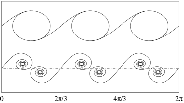
Figure 5: Sketch of the shear-layer patterns, on the developed cylinder $(\theta,z)$, from visual observations. Without annulus (top sketch), the shear produces a triplet of large corotating vortices, corresponding to a $m=3$ mode. In the presence of the equatorial annulus (bottom sketch), the three vortex cores split into corotating pairs: there is a strong energy transfer from the fundamental $m=3$ mode to its first $m=6$ harmonics.

IV.2.3 Scale by scale characterization

\psfrag{d}[c][1.1]{$\overline{\widetilde{\delta}}(k)$}\psfrag{ka}[c][1.1]{$k$ ($D^{-1}$)}\includegraphics[width=216.81pt]{figure6.eps}

Figure 6: (a) Two-dimensional time-averaged Power Spectral Density of instantaneous flows (solid lines) and Power Spectral Density of the corresponding time-averaged flows (dash-dotted lines) for two experiments performed with setup TM73$(+)$, without the annulus ($\scriptstyle\square$) and with the annulus ($\circ$). The PSD are normalized by the total kinetic energy of the mean flow. (b) $\overline{\widetilde{\delta}}(k)$ as function of $k$ for the same setup without ($\scriptstyle\square$) and with annulus ($\circ$). The specific data point $\overline{\widetilde{\delta}}(1/D)$ is represented with a black symbol ($\scriptstyle\blacksquare$). The difference $\Delta\overline{\widetilde{\delta}}(k)$ between the two curves is also displayed (plusses). At high $k$, it is of the order of $\overline{\widetilde{\delta}}(1/D)$ without annulus (see text for details). Wavenumbers are normalized by the PIV window size $D=1.93R$.

By construction, $\bar{\delta}$ accounts for the total fluctuating kinetic energy of the turbulent flow. The use of PSD as an intermediate step to compute $\bar{\delta}$ (cf. Eq. (2)) can provide useful information about the distribution of the energy over the various length scales of the flow as illustrated in Fig. 6. Indeed, in Fig. 6(a), we compare the time-averaged PSD of the instantaneous velocity fields, $\overline{\widetilde{E}}(k)$, to the PSD of the corresponding time averaged field, $\widetilde{E}_{0}(k)$, for the two TM73$(+)$ setups, with and without annulus.

In the spirit of the definitions of turbulent intensity $i$ and of the quantity $\delta$, and because we do access the full spatial spectra, we choose to normalize the PSD by the total kinetic energy of the mean flow. Therefore, the integrals of the displayed curves for the two time-averaged flows are equal to $1$. The wave number $k$ is given by: $k^{2}=k_{r}^{2}+k_{z}^{2}$.

In the time-averaged PSD of the instantaneous flow, the major part of the fluctuating kinetic energy is concentrated close to the forcing scale, where the energy is injected, like in any homogeneous and isotropic turbulent flow. On the contrary, at higher $k$, the slopes of the different PSD are close to $-2$ and larger than the classical $-5/3$ exponent observed for homogeneous isotropic turbulence.

At first sight, the time-averaging removes kinetic energy at all spatial scales. A closer look indicates different relative reductions depending on the presence or the absence of the annulus. At high $k$, the ratio of the PSD of instantaneous to time-averaged flows is of the same order of magnitude for both configuration. However, at low $k$, this ratio is $2$ (resp. $1.2$) without (resp. with) annulus: there are five time less fluctuating low-spatial-frequencies to be averaged when the annulus is inserted meaning that the instantaneous flow is closer to the time-averaged flow.

To quantify more precisely the weight of each scale in $\delta(t)$, we introduce $\widetilde{\delta}(k,t)$ defined as:

$$\widetilde{\delta}(k,t)=\frac{\int^{k}_{0}dk^{\prime}\,\widetilde{E}(k^{\prime},t)}{\int^{\infty}_{0}dk^{\prime}\,\widetilde{E}_{0}(k^{\prime})},$$

so that $\widetilde{\delta}(k,t){\rightarrow}\delta(t)$ when $k\rightarrow\infty$. In Fig. 6(b), $\overline{\widetilde{\delta}}(k)$ is plotted for TM73$(+)$ flows with and without annulus. These curves represent the integral from $0$ to $k$ of the above normalized PSD and they converge towards $\bar{\delta}$ at large $k$.

First of all, we see that the contribution of the 5 first wave numbers, i.e. of spatial modes larger than $D/5\simeq R/10$, is about eighty percents of the total value of $\bar{\delta}$: again, large scales dominate the fluctuations.

Some quantitative analysis can be carried on. We note that the fluctuation level in the first $k=1/D$ mode of the $\overline{\widetilde{\delta}}(k)$ curve without annulus and the difference $\Delta\bar{\tilde{\delta}}$ between the two flows —with and without annulus— are of the same order of magnitude. This is visible in Fig. 6(b), where the $\overline{\widetilde{\delta}}(1/D)$ data point has been emphasized, and has been verified for the three other couples of flows. As described in the previous section, the effect of the annulus can be seen as a spatial filtering of the largest patterns of the flow. The difference between the two curves can be described by a simple empirical protocol. The amount of $\bar{\delta}$ in excess, i.e. $\overline{\widetilde{\delta}}(1/D)\simeq\Delta\bar{\tilde{\delta}}$, is subtracted from the curve $\overline{\widetilde{\delta}}(k)$ without annulus in a geometric progression over $k$, e.g. $\overline{\widetilde{\delta}}(1/D)/2^{k}$ for each wavenumber $k$ starting from $D^{-1}$ or $2D^{-1}$ depending on the configuration. The result is a curve really close to $\overline{\widetilde{\delta}}(k)$ with annulus. The effect of the annulus may thus be seen as a high-pass filtering, which confirms the sketch presented in Fig. 5. Finally, the quantity $\widetilde{\delta}(k,t)$ appears as an efficient tool to track the spectral changes in turbulent scales.

IV.3 Properties of $\delta$ when $f_{1}\neq f_{2}$

As already mentioned in Sec. III.1.3, depending on the value of the rotation number $\theta=(f_{1}-f_{2})/(f_{1}+f_{2})$, the mean von Kármán flow exhibits two different topologies. Indeed, for $|\theta|<\theta_{c}$, the mean flow is composed of two toric recirculation cells separated by an azimuthal shear layer, as for $|\theta|>\theta_{c}$, it is composed of a single recirculation cell ravelet2004 . We have performed a set of experiments for the specific forcing condition TM73$(+)$ with and without annulus, varying $\theta$ from $-1$ to $1$. In this geometry, $\theta_{c}=0.17\pm 0.01$ with annulus and $\theta_{c}\simeq 0.095\pm 0.005$ without annulus. The aim of these experiments is to study the influence of the global rotation and of the transition between the two flow topologies on turbulence intensity.

A way to quantify precisely the turbulent bifurcation of the mean flow occurring at $\theta_{c}$ is to study the position of the azimuthal shear layer that separates the recirculation cells when $|\theta|<\theta_{c}$. A good quantity that allows to localize this position is the zero iso-surface of the stream function $\psi(r,z)$ of the mean flow defined through $(\overline{u_{r}},0,\overline{u_{z}})=\nabla\times(r^{-1}\overline{\psi}\,{\bf e}_{\theta})$ in cylindrical coordinates. Thus, in Figs. 7(a) and (b), we have plotted two measures of the shear layer vertical position at $r=0$, i.e. the stagnation point, and at $r=0.7$ on the side. The discrepancies between these two sets of data renders the fact the shear layer is in general a curved surface expect for the $\theta=0$ configuration. Actually, its vertical position at large $r$ is always closer to the $z=0$ equatorial plane of the vessel than at $r=0$. As $|\theta|$ increases from zero, the shear layer is attracted by the slowest impeller. Without annulus (cf. Fig. 7(a)), it results in a global drift of the shear layer cadot07 accompanied by the appearance of a moderate curvature. With annulus (cf. Fig. 7(b)), the outer edge of the shear layer remains pinned on the annulus whereas its center —the stagnation point— drifts, increasing the layer curvature up to a high level just below $\theta_{c}$: the annulus strongly stabilizes the shear layer near the equatorial plane and maintains it to higher rotation numbers.

At $\theta=\theta_{c}$, we observe a discontinuity of the shear layer vertical position which corresponds to the turbulent bifurcation. The discontinuous bifurcation does not present, in the two studied cases, any hysteresis in $\theta$. However, close to $\theta_{c}$, we can observe transitions between two metastable one cell and two cells states which follow a slow dynamics .

In this section, we first analyze how the parameters $\bar{\delta}$ and $\delta_{2}$ behave with the rotation number. Thereafter, using these tools computed over the two symmetric half of the flow, we analyze how they can also provide a proper characterization of the symmetry breaking.

without annulus	with annulus
\psfrag{p}{shear layer position}\psfrag{a}[c][1.1]{(a)}\psfrag{b}[c][1.1]{(b)}\psfrag{c}[c][1.1]{(c)}\psfrag{d}[c][1.1]{(d)}\psfrag{e}[c][1.1]{(e)}\psfrag{f}[c][1.1]{(f)}\psfrag{d1}[c][1.1]{$\bar{\delta}$}\psfrag{d2}[c][1.1]{$\delta_{2}$}\includegraphics[width=216.81pt]{figure7aceter.eps}	\psfrag{p}{shear layer position}\psfrag{a}[c][1.1]{(a)}\psfrag{b}[c][1.1]{(b)}\psfrag{c}[c][1.1]{(c)}\psfrag{d}[c][1.1]{(d)}\psfrag{e}[c][1.1]{(e)}\psfrag{f}[c][1.1]{(f)}\psfrag{d1}[c][1.1]{$\bar{\delta}$}\psfrag{d2}[c][1.1]{$\delta_{2}$}\includegraphics[width=216.81pt]{figure7bdfter.eps}

Figure 7: (a) and (b), vertical position of the shear layer at $r=0$ on the rotation axis ($\circ$) and at position $r=0.7$ ($\bullet$), (c) and (d) $\bar{\delta}$, and (e) and (f) $\delta_{2}$, as a function of the rotation number $\theta$. Left and right columns correspond respectively to setup TM73$(+)$ without and with annulus. In (a) and (b), the ($\circ$) markers correspond to the stagnation point vertical position. In (c-f), $\bar{\delta}$ and $\delta_{2}$ are computed over the whole flow.

IV.3.1 Variation of $\delta$ with the rotation number

The parameter $\delta$ can be used to study the changes in turbulence intensity related to the turbulent bifurcation undertaken by von Kármán flows at critical $\theta_{c}$. Figs. 7 (c-f) show the variations of $\bar{\delta}$ and $\delta_{2}$, calculated over the whole flow as a function $\theta$.

First of all, for $|\theta|<\theta_{c}$, $\bar{\delta}$ and $\delta_{2}$ are relatively high ($\bar{\delta}\simeq 2$ and $\delta_{2}\simeq 0.2$). This reflects the presence of the highly fluctuating shear layer in the flow bulk. On the contrary, for $|\theta|>\theta_{c}$, i.e. for a large rotation-to-shear rate, $\bar{\delta}$ and $\delta_{2}$ are quite small ($\bar{\delta}\simeq 1.2$ and $\delta_{2}\simeq 0.05$) and are almost independent of $\theta$ . This means that the level of global rotation has no significant influence on the turbulence intensity level unless the mean flow topology changes. Actually, $\bar{\delta}$ and $\delta_{2}$ carefully trace back the flow topology changes induced through the bifurcation at $\pm\theta_{c}$. They might even be used as order parameters of such turbulent bifurcation and they provide a reliable measurement of threshold $\theta_{c}$.

IV.3.2 Effect of the annulus

We have seen how the annulus stabilizes the shear layer and moves the bifurcation threshold. It has also a strong effect on the turbulence level. In Figs. 7 (c-f), we observe that for $|\theta|<\theta_{c}$, when the flow is composed of two counter-rotating toroidal cells, the turbulence level is much larger without than with the annulus: the results for zero-rotation-number (cf. Sec. IV.2) extend to $-\theta_{c}<\theta<\theta_{c}$.

We have already mentioned that this strong reduction in $\bar{\delta}$ and $\delta_{2}$ with the annulus is due to the stabilization, especially at large scales, of the shear layer that is trapped by the annulus. Now, picturing that the flow has a given energy gap to overcome in order to bifurcate from two cells to one cell, the lower level of fluctuations in the case with annulus explains why it is necessary to explore larger $\theta$ before turbulent bifurcation occurs, and then, why $\theta_{c}$ is larger with the annulus. Actually, the annulus is postponing the bifurcation in $\theta$.

For $|\theta|>\theta_{c}$, the low turbulence intensity, almost unchanged at first order, is slightly larger in the presence of the annulus: the one-cell flow is almost insensitive to the annulus presence and the slight increase is probably due to the vertical step flow over the annulus.

IV.3.3 Quantifying the symmetry breaking

For further exploration of the turbulent bifurcation and related symmetry breaking, we now calculate $\bar{\delta}$ and $\delta_{2}$ over half vessels, i.e. on each side of the annulus equatorial plane (cf. Fig. 8).

without annulus	with annulus
\psfrag{a}[c][1.1]{(a)}\psfrag{b}[c][1.1]{(b)}\psfrag{c}[c][1.1]{(c)}\psfrag{d}[c][1.1]{(d)}\psfrag{d1}[c][1.1]{$\bar{\delta}$}\psfrag{d2}[c][1.1]{$\delta_{2}$}\includegraphics[width=216.81pt]{figure8acter.eps}	\psfrag{a}[c][1.1]{(a)}\psfrag{b}[c][1.1]{(b)}\psfrag{c}[c][1.1]{(c)}\psfrag{d}[c][1.1]{(d)}\psfrag{d1}[c][1.1]{$\bar{\delta}$}\psfrag{d2}[c][1.1]{$\delta_{2}$}\includegraphics[width=216.81pt]{figure8bdter.eps}

Figure 8: (a) and (b) $\bar{\delta}$, and (c) and (d) $\delta_{2}$, as a function of the rotation number $\theta$. Left and right columns correspond respectively to setup TM73$(+)$ without and with annulus. ($\blacktriangle$) correspond to $\delta$ computed over the upper half part of the flow as ($\triangledown$) to the lower half part.

Starting from the exact counter-rotating configuration, as $|\theta|$ is increased from zero, $\bar{\delta}$ and $\delta_{2}$ are becoming larger for the half part of the flow corresponding to the slowest impeller and are decreasing for the other half part. This is directly connected with the position of the shear layer which gets closer and closer to the slowest impeller when $\theta$ increases (cf. Figs. 7(a) and (b)). This displacement goes on until the level of fluctuations is strong enough to activate the transition of the flow from two to one cell at $\theta=\theta_{c}$.

Indeed, we clearly see in Figs. 8 the peaks in $\bar{\delta}$ and $\delta_{2}$ that correspond exactly to the bifurcation point $\theta=\theta_{c}$. With the annulus, where the bifurcation is much sharper, one could detect a critical divergence for $(\bar{\delta}-1)$ (cf. Fig. 8(b)).

V Conclusive discussion

We have introduced a new global quantity $\delta$ that characterizes turbulent fluctuations in inhomogeneous anisotropic flows. This time-dependent quantity is based on spatial averages of global velocity fields rather than classical temporal averages of local velocities. We have shown that, generally, properties of $\delta(t)$ seems to be fully provided thanks to only two parameters, its time average $\bar{\delta}$ and variance $\delta_{2}$. These parameters generalize to inhomogeneous anisotropic flows the classical notion of turbulence intensity, based on local, single point measurements.

Properties of $\bar{\delta}$ and $\delta_{2}$ have been experimentally studied in the typical case of the von Kármán flow for different forcing and geometries. We have shown that, in the fully turbulent regime, they are Reynolds independent, like any classical inertial range quantity. However, $\bar{\delta}$ and $\delta_{2}$ depend on forcing and geometry and faithfully reflect major changes in the flow topology. They can therefore be used as a new tool for comparison of different turbulent flow. In the present paper, we provided an example in which $\delta$ is used to characterize the turbulent bifurcation in the von Kármán flow induced through differential rotation of the two impellers. Finally, $\bar{\delta}$ and $\delta_{2}$ are used to characterize the scale by scale energy budget as a function of the forcing mode as well as the transition between the two flow topologies.

Another interesting application would be the study of the generation of magnetic field by a turbulent flow, the so-called dynamo instability. This problem has attracted recently a lot of experimental attention gailitis01 ; stieglitz01a ; monchaux2007 . In the case where the corresponding turbulent flow has a non-zero mean value, the dynamo instability may be seen as a classical instability problem, governed by the mean flow and the fluctuations leprovost2005 ; LavalDyn ; petrelis06b . A natural question in this case is therefore how to quantify the relative level of fluctuations, and the deviations from the mean flow they induce, so as to implement efficient control strategies to decrease or increase their influence. Since our global parameter quantify the difference between the instantaneous and the mean flow, they are natural candidate to discriminate between different dynamos. This has been recently illustrated in numerical simulations of Taylor-Green flow dubrulle07 . No equivalent quantitative analysis has been performed for experimental dynamos. However, among these successful experimental dynamos, we can suspect that the Karlsruhe stieglitz01a and Riga gailitis01 flows are characterized by values of $\delta$ lower than in von Kármán flows. In the future, we plan to use these parameters for the analysis of recent results of the von Kármán Sodium (VKS) experiment.

Appendix A Convergence towards the mean flow

\psfrag{d}[c][1.1]{$\bar{\delta}(N)-1$}\includegraphics[width=195.12767pt]{figure9.eps}

Figure 9: $\bar{\delta}-1$ computed with velocity fields averaged over $N$ instantaneous fields for various setups : TM73$(-)$, without the annulus ($\scriptstyle\blacksquare$) and with the annulus ($\bullet$) and TM73$(+)$, without annulus ($\scriptstyle\square$) and with annulus ($\circ$). A guide to the eye for the $N^{-1}$ dependency is plotted with a dotted line.

As we have seen in Sec. II, the parameter $\bar{\delta}$ can be seen as the average square distance between the instantaneous and the time averaged velocity fields. Therefore, we can use a slight modification of $\bar{\delta}$ to study the convergence towards the mean flow through statistical averaging. For this, we define $V(N,t)$ the velocity field averaged around time $t$ over $N$ instantaneous fields. $N<N_{max}$ where $N_{max}=5000$ is the total number of instantaneous fields. From a practical point of view, $V(N_{max})=\overline{V(t)}$. Then, we define:

$$\bar{\delta}(N)=\frac{\overline{\langle V^{2}(N,t)\rangle}}{\langle\overline{V}^{2}\rangle}.$$ (3)

With this definition, $\bar{\delta}(1)=\bar{\delta}$ and $\bar{\delta}(N_{max})=1$. Moreover, $\bar{\delta}(N)-1$ measures the average square distance between the partially averaged field $V(N)$ and the mean flow $\overline{V}$, so that its variations with $N$ can be used to study the convergence towards the mean flow. We can see in Fig. 9 that this square distance, $\bar{\delta}(N)-1$, decreases as $N^{-1}$, at least at large $N$, what is typical of an uncorrelated fluctuating quantity. However, for the negative-rotation-sense-with-annulus case, the $N^{-1}$ dependency is observed only at $N$ larger than $100$. Actually, in that particular setup, we have observed, by means of bubble seeding (cf. end of Sec. IV.2.2), that even if the largest structures of the shear layer where removed by the annulus, a pair of coupled vortices appeared. These vortices are smaller than those we observe without the annulus, but their long time coherent precessing must induce long time correlations that slow down the decrease of $\bar{\delta}(N)$.

References

- [1] U. Frisch. Turbulence-The Legacy of A. N. Kolmogorov. Cambridge University Press, Cambridge, 1995.
- [2] O. Cadot, S. Douady, and Y. Couder. Characterization of the low-pressure filaments in a three-dimensional turbulent shear flow. Phys. Fluids, 7:630–646, 1995.
- [3] R. Labbé, J.-F. Pinton, and S. Fauve. Study of the von Kármán flow between coaxial corotating disks. Phys. Fluids, 8(4):914–922, 1996.
- [4] N. Mordant, J.-F. Pinton, and F. Chillà. Characterization of turbulence in a closed flow. J. Phys. II, 7:1729–1742, 1997.
- [5] F. Ravelet, L. Marié, A. Chiffaudel, and F. Daviaud. Multistability and memory effect in a highly turbulent flow: Experimental evidence for a global bifurcation. Phys. Rev. Lett., 93:164501, 2004.
- [6] C. Nore, F. Moisy, and L. Quartier. Experimental observation of near-heteroclinic cycles in the von Kármán swirling flow. Phys. Fluids, 17:064103, 2005.
- [7] J. Maurer, P. Tabeling, and G. Zocchi. Statistics of turbulence between two counterrotating disks in low-temperature helium gas. Europhys. Lett., 26:31–36, 1994.
- [8] P. Tabeling, G. Zocchi, F. Belin, J. Maurer, and H. Willaime. Probability density functions, skewness, and flatness in large Reynolds number turbulence. Phys. Rev. E, 53:1613–1621, 1996.
- [9] A. Arneodo, C. Baudet, F. Belin, R. Benzi, B. Castaing, B. Chabaud, R. Chavarria, S. Ciliberto, R. Camussi, F. Chillà, B. Dubrulle, Y. Gagne, B. Hebral, J. Herweijer, M. Marchand, J. Maurer, J.-F. Muzy, A. Naert, A. Noullez, J. Peinke, F. Roux, P. Tabeling, W. van de Water, and H. Willaime. Structure functions in turbulence, in various flow configurations, at Reynolds number between 30 and 5000, using extended self-similarity. Europhys. Lett., 34:411–416, 1996.
- [10] L. Marié. Transport de moment cinétique et de champ magnétique par un écoulement tourbillonaire turbulent: influence de la rotation. PhD thesis, Université Paris VII, 2003.
- [11] L. Marié and F. Daviaud. Experimental measurement of the scale-by-scale momentum transport budget in a turbulent shear flow. Phys. Fluids, 16:457, 2004.
- [12] F. Ravelet, A. Chiffaudel, F. Daviaud, and J. Leorat. Toward an experimental von Kármán dynamo: Numerical studies for an optimized design. Phys. Fluids, 17:117104, 2005.
- [13] R. Monchaux, F. Ravelet, B. Dubrulle, A. Chiffaudel, and F. Daviaud. Properties of steady states in turbulent axisymmetric flows. Phys. Rev. Lett., 96:124502, 2006.
- [14] F. Ravelet, A. Chiffaudel, and F. Daviaud. Supercritical transition to turbulence in an inertially driven von Kármán closed flow. J. Fluid Mech., 601:339, 2008.
- [15] R. Monchaux. Mécanique statistique et effet dynamo dans un écoulement de von Kármán turbulent. PhD thesis, Université Paris VII, 2007.
- [16] J.-P. Laval, P. Blaineau, N. Leprovost, B. Dubrulle, and F. Daviaud. Influence of turbulence on the dynamo threshold. Phys. Rev. Lett., 96(20):204503, 2006.
- [17] O. Cadot and O. Le Maitre. The turbulent flow between two rotating stirrers: similarity laws and transitions for the driving torques fluctuations. Eur. J. Mech. B, 26:258, 2007.
- [18] A. Gailitis, O. Lielausis, E. Platacis, S. Dement’ev, A. Cifersons, G. Gerbeth, T. Gundrum, F. Stefani, M. Christen, and G. Will. Magnetic Field Saturation in the Riga Dynamo Experiment. Phys. Rev. Lett., 86:3024–3027, 2001.
- [19] R. Stieglitz and U. Müller. Experimental demonstration of a homogeneous two-scale dynamo. Phys. Fluids, 13:561–564, 2001.
- [20] R. Monchaux, M. Berhanu, M. Bourgoin, M. Moulin, Ph. Odier, J.-F. Pinton, R. Volk, S. Fauve, N. Mordant, F. Pétrélis, A. Chiffaudel, F. Daviaud, B. Dubrulle, C. Gasquet, L. Marié, and F. Ravelet. Generation of magnetic field by dynamo action in a turbulent flow of liquid sodium. Phys. Rev. Lett., 98:44502, 2007.
- [21] N. Leprovost and B. Dubrulle. The turbulent dynamo as an instability in a noisy medium. Eur. Phys. J. B, 44:395, 2005.
- [22] F. Pétrélis and S. Fauve. Inhibition of the dynamo effect by phase fluctuations. Europhys. Lett., 76:602–608, 2006.
- [23] B. Dubrulle, P. Blaineau, O. Mafra Lopes, F. Daviaud, J.-P. Laval, and R. Dolganov. Bifurcations and dynamo action in a Taylor-Green flow. New J. Phys., 9:308, 2007.
- [24] L. Marié, J. Burguete, F. Daviaud, and J. Léorat. Numerical study of homogeneous dynamo based on experimental von Kármán type flows. Eur. Phys. J. B, 33:469, 2003.
- [25] M. Bourgoin, L. Marié, F. Pétrélis, C. Gasquet, A. Guigon, J.-B. Luciani, M. Moulin, F. Namer, J. Burguete, A. Chiffaudel, F. Daviaud, S. Fauve, P. Odier, and J.-F. Pinton. MHD measurements in the von Kármán sodium experiment. Phys. Fluids, 14:3046, 2002.