Price dynamics in a strategic model of trade between two regions

Abstract

This paper develops a strategic model of trade between two regions in which, depending on the relation among output, financial resources and transportation costs, the adjustment of prices towards an equilibrium is studied. We derive conditions on the relations among output and financial resources which produce different types of Nash equilibria. The paths obtained in the process of converging toward a steady state for prices under discrete-time and continuous-time dynamics are derived and compared. It turns out that the results in the two cases differ substantially. Some of the effects of random disturbances on the price dynamics in continuous time are also studied.

1 Introduction

The present work develops a model of trade between two regions in which, depending on the relation among output, financial resources and transportation costs, the adjustment of prices towards a steady state is studied. We assume that there is one type of traded good and local producers can supply only a fixed amount of this traded good, which cannot be stored for future consumption. As usual, prices change to balance supply and demand. In the chosen setup, the evolution of prices according to an exogenous rule is studied, starting from pre-specified initial conditions. More specifically, whenever there are unsold quantities left, the price is decreased proportionally and when there are local financial resources unspent, the price is increased proportionally. This allows us to abstract away from producer behaviour and focus exclusively on consumers’ decisions. The representative consumers in the two regions seek to maximize their per-period utility in a strategic situation arising from the need to compete for scarce resources. We utilize the concept of Nash equilibrium to characterize optimal behaviour in the game theoretic interaction. This equilibrium concept has the advantage of delivering consistent predictions of the outcomes of a game, assuming that each player takes into account the other players’ optimizing decisions (see Ch.1 in [3] for a more detailed discussion of the concept).

Under the above setup we derive conditions on the relations among quantities produced and financial resources, for which different types of Nash equilibria arise. We also compute the paths obtained in the process of prices converging toward a steady state. In certain cases the laws governing price dynamics in discrete time lead to a zero price in one of the regions, which can be interpreted as a breakdown of economic activity in the region. Such pathologies do not arise in the case of continuous-time price dynamics, where the continuous nature of the adjustment process provides a natural balancing mechanism against degenerate stationary points for prices. The stability properties of the stationary points in the continuous-time case are proved analytically and illustrated through the behaviour of the phase trajectories of the system in the presence of stochastic disturbances.

The paper is organized as follows. Section 2 introduces the model and key notational conventions. Section 3 shows the existence and form of Nash equilibria for the model under discussion. Section 4 calculates and compares the dynamics governing prices in discrete time, while section 5 presents the counterpart analysis in the continuous-time case. The proofs of the results from section 4 are provided in the appendix. Section 6 contains the results of some simulations for the continuous-time case with stochastic shocks. Partial announcements of the results reported in this paper appeared in [4] and [7].

2 The model

We consider the consumption decisions of two economic agents occupying distinct spatial locations, called region $I$ and $II$, respectively. The consumer in region $I$ (or, shortly, consumer $I$) exogenously receives money income $Y_{1}>0$ in each period. Similarly, the consumer in region $II$ (consumer $II$) receives money income $Y_{2}>0$. For each period $t$, in region $i$, $i=1,2$, a fixed quantity $q_{i}>0$ of a certain good is supplied at a price $p_{i,t}$. The consumers place orders for the desired quantities in each region, observing their budget constraints and incurring symmetric transportation costs $\rho>0$ per unit of shipment from the ‘‘foreign’’ region. Each consumer attempts to maximize their total consumption for the current period. Consumers can be considered myopic in that they do not optimize their consumption over a specified time horizon but their decisions are confined only to the current period.

In cases when total orders for the respective region exceed the quantity available, the following distribution rule is applied: first, the order of the local consumer is executed to the extent possible and then the remaining quantity, if any, is allocated to the consumer from the other region. We sometimes refer to this distribution scheme and its consequences as local dominance. It is clear then that the choice of orders to be placed has a strategic element to it, since the actual quantity received by the consumer depends on the choices made by the counterpart in the other region. The agents are assumed to have complete knowledge of all the relevant aspects of the situation under discussion.

More formally, for each period $t$ we model the above situation as a static noncooperative game of complete information. Denote by $\alpha$ and $\beta$ the orders placed by consumer $I$ in region $I$ and $II$, respectively. In an analogous manner, $\gamma$ and $\delta$ stand for the orders of consumer $II$ in regions $I$ and $II$, all orders obviously being nonnegative quantities. In period $t$ consumer $I$’s strategy space $S_{1}$ is determined by the budget constraint and the nonnegativity restrictions on the orders:

(2.1) $$S_{1}=\{(\alpha,\beta)\in\mathbb{R}^{2}|\alpha p_{1,t}+\beta(p_{2,t}+\rho)\leq Y_{1},\quad\alpha,~{}\beta\geq 0\}.$$

Consumer $II$’s strategy space in period $t$ is

(2.2) $$S_{2}=\{(\gamma,\delta)\in\mathbb{R}^{2}|\gamma(p_{1,t}+\rho)+\delta p_{2,t}\leq Y_{2},\quad\gamma,~{}\delta\geq 0\}.$$

Below we adopt the shorthand $p_{1,t}^{\prime}:=p_{1,t}+\rho$ and $p_{2,t}^{\prime}:=p_{2,t}+\rho$. We also omit the subscript $t$ whenever it is evident from the context or irrelevant.

The payoff function for consumer $I$ is given by

(2.3) $$\begin{split}P_{1}(\alpha,\beta,\gamma,\delta)=&\min(\alpha,~{}q_{1})+\min(\beta,~{}q_{2}-\min(\delta,~{}q_{2}))\equiv\\ \equiv&\min(\alpha,~{}q_{1})+\min(\beta,~{}\max(0,~{}q_{2}-\delta))\end{split}$$

and that for consumer $II$ by

(2.4) $$\begin{split}P_{2}(\alpha,\beta,\gamma,\delta)=&\min(\gamma,~{}q_{1}-\min(\alpha,~{}q_{1}))+\min(\delta,~{}q_{2})\equiv\\ \equiv&\min(\delta,~{}q_{2})+\min(\gamma,~{}\max(0,~{}q_{1}-\alpha)).\end{split}$$

Any unspent fraction of the current-period income is assumed to perish and consequently the accumulation of stocks of savings is not allowed in the model. Similarly, the goods available each period cannot be stored for future consumption. Let $q_{i}^{cons}$ denote the total amount consumed in region $i$ and $Y_{i}^{res}$ stand for the part of the region $i$’s income not spent in the other region. In other words, $q_{1}^{cons}:=\alpha_{0}+\gamma_{0}$, $q_{2}^{cons}:=\beta_{0}+\delta_{0}$, $Y_{1,t}^{res}:=Y_{1}-p^{\prime}_{2,t}\beta_{0}$ and $Y_{2,t}^{res}:=Y_{2}-p^{\prime}_{1,t}\gamma_{0}$.

There are two mutually exclusive situations leading to an adjustment in prices. First, if the quantity available in the respective region has not been entirely consumed, prices are adjusted downwards. In discrete time this is captured by the equation

(2.5) $$\frac{p_{i,t}-p_{i,t+1}}{p_{i,t}}=\frac{q_{i}-q_{i,t}^{cons}}{q_{i}}\textrm{ or }p_{i,t+1}q_{i}=p_{i,t}q_{i,t}^{cons}.$$

Clearly, if $q_{i}^{cons}=0$, then $p_{i,t+1}=0$. Second, if $Y_{i}^{res}$ is not entirely exhausted in absorbing local supply, which can be expressed in value terms as $p_{i}q_{i}$, then the price $p_{i,t}$ is adjusted upwards to $p_{i,t+1}$ to ensure residual income exhaustion:

(2.6) $$\frac{p_{i,t+1}-p_{i,t}}{p_{i,t}}=\frac{Y_{i,t}^{res}-p_{i,t}q_{i}}{p_{i,t}q_{i}}\textrm{ or }p_{i,t+1}q_{i}=Y_{i,t}^{res}.$$

Obviously the fraction of $Y_{i}$ spent on the ‘‘foreign’’ market cannot be attracted back for domestic consumption if local prices are increasing. Later we formally prove the claim that the two situations leading to price adjustment cannot occur simultaneously. As usual, we consider prices in a steady state if the rules given by equations (2.5) and (2.6) do not lead to a change in prices.

For the above model we are interested in two main questions. First, it would be desirable to establish the existence of a Nash equilibrium for the one-period game and specify it in closed form. Second, one would like to be able to trace out the price dynamics entailed by a sequence of one-period games for a given set of initial conditions $p_{1,0},~{}p_{2,0},~{}q_{1},~{}q_{2},~{}Y_{1},~{}Y_{2}$ and $\rho$, and characterize their properties.

3 Existence and form of equilibrium

In this section we study the existence and properties of the most popular equilibrium concept – that of Nash equilibrium – for the model specified above,for a fixed time period $t$. Our basic tool for establishing existence is a theorem [2, p. 72] asserting that at least one Nash equilibrium exists for a game of complete information for which:

• the strategy spaces of all players are compact and convex subsets of $\mathbb{R}^{m}$;

• all payoff functions are defined, continuous and bounded over the strategy space of the game, and

• any payoff function is quasiconcave in the player’s own feasible strategies for a fixed strategy profile of the opponents.

We remind the reader that a function $f:X\rightarrow\mathbb{R}$ is called quasiconcave if for any $x,y\in X$ we have $f(\lambda x+(1-\lambda)y)\geq\min\{f(x),f(y)\}$ for all $\lambda\in(0,1)$.

Properties (a) and (b) are immediately verified for our model when the prices $p_{i}$ are positive. (If a price is zero, economically plausible restrictions are imposed on the model in order to ensure that the above properties hold in this case as well; see SR3.) To establish property (c) note that the payoff function for each consumer is separable in the consumer’s orders and each component of the sum in the payoff is a concave function in the respective order. These observations entail the concavity and hence the quasiconcavity of the payoffs.

Since all the hypotheses of the existence theorem are satisfied for our model, it has at least one Nash equilibrium. We proceed to compute the Nash equilibria for all possible configurations of $Y_{1},~{}Y_{2},~{}q_{1},~{}q_{2},~{}p_{1},~{}p_{2}$ and $\rho$. To this end, we derive the best-reply correspondences (see [2, pp. 69-75] ) for the two consumers. We remind that these correspondences are defined as follows. Let us denote

$$u_{1}(\alpha,\beta)=P_{1}(\alpha,\beta,\gamma,\delta)$$

for fixed values of $(\gamma,\delta)\in S_{2}$ and

$$u_{2}(\gamma,\delta)=P_{2}(\alpha,\beta,\gamma,\delta)$$

for fixed values of $(\alpha,\beta)\in S_{1}$. Let $(\bar{\alpha}(\gamma,\delta),\bar{\beta}(\gamma,\delta))$ be defined as

$$\operatorname*{argmax}_{(\alpha,\beta)\in S_{1}}u_{1}(\alpha,\beta)$$

and, similarly, let $(\bar{\gamma}(\alpha,\beta),\bar{\delta}(\alpha,\beta))$ be defined as

$$\operatorname*{argmax}_{(\gamma,\delta)\in S_{2}}u_{2}(\gamma,\delta).$$

The (multivalued) correspondence $(\alpha,\beta,\gamma,\delta)\mapsto(\bar{\alpha},\bar{\beta},\bar{\gamma},\bar{\delta})$ is called best-reply correspondence for the problem, with $r_{1}(\gamma,\delta):=(\bar{\alpha},\bar{\beta})$ and $r_{2}(\alpha,\beta):=(\bar{\gamma},\bar{\delta})$ being the best-reply functions for consumers $I$ and $II$, respectively.

The derivation of the best-reply correspondences is straightforward and we omit the details, presenting only the end-results. Table 3.1 presents the best-reply correspondence for consumer $I$ and Table 3.2 shows the best-reply correspondence for consumer II. For simplicity in the tables we use $\alpha$ instead of $\bar{\alpha}$ etc. for the equilibrium values. We note in advance that in the course of the price adjustment process one of the prices can become zero, in which case the best reply correspondences take a different form (see Tables 3.3 and 3.4 below).

	$\mathbf{A:\frac{Y_{1}}{p_{1}}>q_{1}}$		$\mathbf{B:\frac{Y_{1}}{p_{1}}\leq q_{1}}$
$\mathbf{I.~{}q_{2}-\boldsymbol{\delta}\leq 0}$	$q_{1}\leq\alpha\leq\frac{Y_{1}}{p_{1}},~{}0\leq\beta\leq\frac{Y_{1}-p_{1}\alpha}{p_{2}^{\prime}}$, SR1: $\alpha=q_{1}$, $\beta=0$		$\alpha=\frac{Y_{1}}{p_{1}},~{}\beta=0$
	$\mathbf{A_{1}:0<q_{1}<\frac{Y_{1}-p_{2}^{\prime}(q_{2}-\boldsymbol{\delta})}{p_{1}}}$	$\mathbf{A_{2}:\frac{Y_{1}-p_{2}^{\prime}(q_{2}-\boldsymbol{\delta})}{p_{1}}\leq q_{1}<\frac{Y_{1}}{p_{1}}}$
		$\mathsf{(1)}:\alpha=q_{1},~{}\beta=\frac{Y_{1}-p_{1}q_{1}}{p_{2}^{\prime}}$	$\mathsf{(1)}:\alpha=\frac{Y_{1}}{p_{1}},~{}\beta=0$
$\mathbf{II.~{}q_{2}-\boldsymbol{\delta}\in\left(0,\frac{Y_{1}}{p_{2}^{\prime}}\right]}$	$q_{1}\leq\alpha\leq\frac{Y_{1}-p_{2}^{\prime}(q_{2}-\delta)}{p_{1}}$	$\mathsf{(2)}:\frac{Y_{1}-p_{2}^{\prime}(q_{2}-\delta)}{p_{1}}\leq\alpha\leq q_{1},~{}$	$\mathsf{(2)}:\alpha=\frac{Y_{1}-p_{2}^{\prime}\beta}{p_{1}},$
	$q_{2}-\delta\leq\beta\leq\frac{Y_{1}-p_{1}\alpha}{p_{2}^{\prime}}$	$\beta=\frac{Y_{1}-p_{1}\alpha}{p_{2}^{\prime}}$, SR2: as in (1)	$0\leq\beta\leq\frac{p_{2}^{\prime}(q_{2}-\delta)}{p_{1}}$, SR2: as in (1)
	SR1: $\alpha=q_{1}$, $\beta=q_{2}-\delta$	$\mathsf{(3)}:\alpha=\frac{Y_{1}-p_{2}^{\prime}(q_{2}-\delta)}{p_{1}},$	$\mathsf{(3)}:\alpha=\frac{Y_{1}-p_{2}^{\prime}(q_{2}-\delta)}{p_{1}},$
		$\beta=q_{2}-\delta$	$\beta=q_{2}-\delta$
	$\mathsf{(1)}:\alpha=q_{1},~{}\beta=\frac{Y_{1}-p_{1}q_{1}}{p_{2}^{\prime}}$		$\mathsf{(1)}:\alpha=\frac{Y_{1}}{p_{1}},~{}\beta=0$
$\mathbf{III.~{}q_{2}-\boldsymbol{\delta}>\frac{Y_{1}}{p_{2}^{\prime}}}$	$\mathsf{(2)}:0\leq\alpha\leq q_{1},~{}\beta=\frac{Y_{1}-p_{1}\alpha}{p_{2}^{\prime}}$, SR2: as in (1)		$\mathsf{(2)}:0\leq\alpha\leq\frac{Y_{1}}{p_{1}},$
	$\mathsf{(3)}:\alpha=0,~{}\beta=\frac{Y_{1}}{p_{2}^{\prime}}$		$\beta=\frac{Y_{1}-p_{1}\alpha}{p_{2}^{\prime}}$, SR2: as in (1)
			$\mathsf{(3)}:\alpha=0,~{}\beta=\frac{Y_{1}}{p_{2}^{\prime}}$
Shorthand notation used: $\mathsf{(1)}$ for $\mathsf{p_{1}<p_{2}^{\prime}}$, $\mathsf{(2)}$ for $\mathsf{p_{1}=p_{2}^{\prime}}$ and $\mathsf{(3)}$ for $\mathsf{p_{1}>p_{2}^{\prime}}$
Whenever the shorthand notation is not employed, the result should be taken to apply to each of the three cases.

Table 3.1: Best-reply correspondence for consumer $I$.

	$\mathbf{A:\frac{Y_{2}}{p_{2}}>q_{2}}$		$\mathbf{B:\frac{Y_{2}}{p_{2}}\leq q_{2}}$
$\mathbf{I.~{}q_{1}-\boldsymbol{\alpha}\leq 0}$	$0\leq\gamma\leq\frac{Y_{2}-p_{2}q_{2}}{p_{1}^{\prime}},~{}q_{2}\leq\delta\leq\frac{Y_{2}-p_{1}^{\prime}\gamma}{p_{2}}$, SR1: $\gamma=0$, $\delta=q_{2}$		$\gamma=0,~{}\delta=\frac{Y_{2}}{p_{2}}$
	$\mathbf{A_{1}:0<q_{2}<\frac{Y_{2}-p_{1}^{\prime}(q_{1}-\boldsymbol{\alpha})}{p_{2}}}$	$\mathbf{A_{2}:\frac{Y_{2}-p_{1}^{\prime}(q_{1}-\boldsymbol{\alpha})}{p_{2}}\leq q_{2}<\frac{Y_{2}}{p_{2}}}$
		$\mathsf{(1)}:\gamma=\frac{Y_{2}-p_{2}q_{2}}{p_{1}^{\prime}},~{}\delta=q_{2}$	$\mathsf{(1)}:\gamma=0,~{}\delta=\frac{Y_{2}}{p_{2}}$
$\mathbf{II.~{}q_{1}-\boldsymbol{\alpha}\in\left(0,\frac{Y_{2}}{p_{1}^{\prime}}\right]}$	$q_{1}-\alpha\leq\gamma\leq\frac{Y_{2}-p_{2}q_{2}}{p_{1}^{\prime}}$	$\mathsf{(2)}:\frac{Y_{2}-p_{2}q_{2}}{p_{1}^{\prime}}\leq\gamma\leq q_{1}-\alpha,~{}$	$\mathsf{(2)}:0\leq\gamma\leq q_{1}-\alpha,$
	$q_{2}\leq\delta\leq\frac{Y_{2}-p_{1}^{\prime}\gamma}{p_{2}}$	$\delta=\frac{Y_{2}-p_{1}^{\prime}\gamma}{p_{2}}$, SR2: as in (1)	$\delta=\frac{Y_{2}-p_{1}^{\prime}\gamma}{p_{2}}$, SR2: as in (1)
	SR1: $\gamma=q_{1}-\alpha$, $\delta=q_{2}$	$\mathsf{(3)}:\gamma=q_{1}-\alpha,$	$\mathsf{(3)}:\gamma=q_{1}-\alpha,$
		$\delta=\frac{Y_{2}-p_{1}^{\prime}\gamma}{p_{2}}$	$\delta=\frac{Y_{2}-p_{1}^{\prime}\gamma}{p_{2}}$
	$\mathsf{(1)}:\gamma=\frac{Y_{2}-p_{2}q_{2}}{p_{1}^{\prime}},~{}\delta=q_{2}$		$\mathsf{(1)}:\gamma=0,~{}\delta=\frac{Y_{2}}{p_{2}}$
$\mathbf{III.~{}q_{1}-\boldsymbol{\alpha}>\frac{Y_{2}}{p_{1}^{\prime}}}$	$\mathsf{(2)}:\frac{Y_{2}-p_{2}q_{2}}{p_{1}^{\prime}}\leq\gamma\leq\frac{Y_{2}}{p_{1}^{\prime}},~{}\delta=\frac{Y_{2}-p_{1}^{\prime}\gamma}{p_{2}}$, SR2: as in (1)		$\mathsf{(2)}:0\leq\gamma\leq\frac{Y_{2}}{p_{1}^{\prime}},$
	$\mathsf{(3)}:\gamma=\frac{Y_{2}}{p_{1}^{\prime}},~{}\delta=0$		$\delta=\frac{Y_{2}-p_{1}^{\prime}\gamma}{p_{2}}$, SR2: as in (1)
			$\mathsf{(3)}:\gamma=\frac{Y_{2}}{p_{1}^{\prime}},~{}\delta=0$
Shorthand notation used: $\mathsf{(1)}$ for $\mathsf{p_{1}^{\prime}>p_{2}}$, $\mathsf{(2)}$ for $\mathsf{p_{1}^{\prime}=p_{2}}$ and $\mathsf{(3)}$ for $\mathsf{p_{1}^{\prime}<p_{2}}$
Whenever the shorthand notation is not employed, the result should be taken to apply to each of the three cases.

Table 3.2: Best-reply correspondence for consumer $II$.

Several comments are in order with respect to the Tables 3.1 and 3.2. Because of the presence of the parameters $(q_{i},Y_{i},p_{i},\rho)$, as well as the different feasible values of the fixed variables, the procedure for maximizing $u_{i},~{}i=1,2,$ can be decomposed into different cases in a natural manner. For example, to find $\max u_{1}$ we get rid of $\max(0,q_{2}-\delta)$ by successively analyzing the two cases $q_{2}\leq\delta$ and $q_{2}>\delta$. The second case in turn decomposes into two subcases depending on whether the quantity $q_{2}-\delta$ is smaller or greater than the maximal feasible value $Y_{1}/p^{\prime}_{2}$ of $\beta$. For $\alpha$, which we compare with $q_{1}$, the geometry of the feasible set depends on, first, the size of the difference $q_{1}-\alpha_{0}$, where $\alpha_{0}$ is determined from the condition $Y_{1}=p_{1}\alpha_{0}+p^{\prime}_{2}(q_{2}-\delta)$, assuming $q_{2}-\delta\in(0,Y_{1}/p^{\prime}_{2})$ and, second, by the ratio between the size of local supply $q_{1}$ and the maximum purchasing power of local income, $Y_{1}/p_{1}$.

With the aid of the best-reply correspondences we can compute the Nash equilibria for the game as solutions to a system of equations. However, uniqueness is not guaranteed in this model and we therefore have to resort to additional rules for equilibrium selection in order to choose a single equilibrium. To this end we define the following supplementary selection rules (SR), which we deem logical from a practical viewpoint:

• (Expenditure minimization) For a set of Nash equilibria yielding the same utility we select the one minimizing the expenditures made. (The expenditures made by the first consumer are $p_{1}\alpha+p^{\prime}_{2}\beta$ and those made by the second consumer are $p^{\prime}_{1}\gamma+p_{2}\delta$.)

• (Home bias) If more than one Nash equilibrium with the same utility can be obtained with the same (minimal) expenditure, then we select the one in which consumers receive the maximum amount possible in their own region in preference over the ‘‘foreign’’ consumer. (I.e. if for the first market we have $p_{1}\alpha+p^{\prime}_{2}\beta=const$ for more than one point $(\alpha,\beta)$, we choose the point with the largest value of $\alpha$. We proceed analogously for the second market.)

• (Free disposal) In the degenerate case when a price is equal to zero, we assume that the actual amount bought is equal to the quantity available in the respective region.

SR3 points to a modification in the best-reply correspondences required in the degenerate case of a zero price. If $p_{1}=0$, i.e. $p^{\prime}_{1}=\rho$, Table 3.2 should be modified into a table identical to the former with $p^{\prime}_{1}=\rho$ and $p_{2}>0$. Table 3.1 should be replaced by Table 3.3.

Subcase	$\boldsymbol{(\bar{\alpha},\bar{\beta})}$	Selection as per SR3
$\mathbf{q_{2}-\boldsymbol{\delta}\leq 0}$	$q_{1}\leq\alpha$	$(q_{1},0)$
	$0\leq\beta\leq\frac{Y_{1}}{p^{\prime}_{2}}$
$\mathbf{0<q_{2}-\boldsymbol{\delta}\leq\frac{Y_{1}}{p^{\prime}_{2}}}$	$q_{1}\leq\alpha$	$(q_{1},q_{2}-\delta)$
	$q_{2}-\delta\leq\beta\leq\frac{Y_{1}}{p^{\prime}_{2}}$
$\mathbf{\frac{Y_{1}}{p^{\prime}_{2}}<q_{2}-\boldsymbol{\delta}}$	$q_{1}\leq\alpha$	$\left(q_{1},\frac{Y_{1}}{p^{\prime}_{2}}\right)$
	$\beta=\frac{Y_{1}}{p^{\prime}_{2}}$

Table 3.3: Modification of Table 3.1 for the degenerate case $p_{1}=0$.

Subcase	$\boldsymbol{(\bar{\gamma},\bar{\delta})}$	Selection as per SR3
$\mathbf{q_{1}-\boldsymbol{\alpha}\leq 0}$	$0\leq\gamma\leq\frac{Y_{2}}{p^{\prime}_{1}}$	$(0,q_{2})$
	$q_{2}\leq\delta$
$\mathbf{0<q_{1}-\boldsymbol{\alpha}\leq\frac{Y_{2}}{p^{\prime}_{1}}}$	$q_{1}-\alpha\leq\gamma\leq\frac{Y_{2}}{p^{\prime}_{1}}$	$(q_{1}-\alpha,q_{2})$
	$q_{2}\leq\delta$
$\mathbf{\frac{Y_{2}}{p^{\prime}_{1}}<q_{1}-\boldsymbol{\alpha}}$	$\gamma=\frac{Y_{2}}{p^{\prime}_{1}}$	$\left(\frac{Y_{2}}{p^{\prime}_{1}},q_{2}\right)$
	$q_{2}\leq\delta$

Table 3.4: Modification of Table 3.2 for the degenerate case $p_{2}=0$.

If $p_{2}=0$, i.e. $p^{\prime}_{2}=\rho$, Table 3.1 should be replaced by an identical table with $p^{\prime}_{2}=\rho,~{}p_{1}=0$ and Table 3.2 should be replaced by Table 3.4.

In an analogous manner, by using SR1 and SR2 we can dispose of the multiplicity of solutions and arrive at a unique Nash equilibrium $(\alpha,\beta,\gamma,\delta)$, as reflected in Tables 3.1 and 3.2. The latter can be obtained as a solution of the system

(3.1) $$\left\{\begin{array}[]{ccc}\bar{\alpha}(\gamma,\delta)&=&\alpha\\ \bar{\beta}(\gamma,\delta)&=&\beta\\ \bar{\gamma}(\alpha,\beta)&=&\gamma\\ \bar{\delta}(\alpha,\beta)&=&\delta,\end{array}\right.$$

which we derive explicitly in section 4 and in the appendix.

4 Price dynamics in the discrete-time case

By definition, a steady state (point of equilibrium, p.e.) for the prices $p_{i}$ is the value for which consumption (as given by the Nash equilibrium $(\alpha,\beta,\gamma,\delta)$, NE for brevity) leads to a complete depletion of both the available quantities $q_{i}$ of the good and the financial resources $Y_{i}$. In other words, for $q_{i}$ and $Y_{i}$ exogenously given, we have $\alpha+\gamma=q_{1}$, $\beta+\delta=q_{2}$, $p_{1}\alpha+p^{\prime}_{2}\beta=Y_{1}$, $p^{\prime}_{1}\gamma+p_{2}\delta=Y_{2}$. As a result prices are not adjusted for the next period but retain their current values.

Naturally, if the initial values of prices are not a p.e., they are corrected prior to next period’s consumption, as described above. The present section aims to characterize the evolution of prices for all possible values of $Y_{i}$ (for fixed $q_{i},\rho>0$). For this purpose, it is convenient to present the results in $Y_{1}$-$Y_{2}$ space. In accordance with the different cases presented in Tables 3.1 and 3.2, we partition (by means of a set of lines and additional restrictions) the nonnegative quadrant of the plane into disjoint subsets of points $(\tilde{Y}_{1},\tilde{Y}_{2})$ for which a unique NE exists. Each NE corresponding to an element of this partition is presented as a closed-form expression involving the exogenous parameters. However, the partition itself (or, respectively, the set of lines), crucially depends on the values of $p_{i}$. After prices have been adjusted, the point $(Y_{1},Y_{2})$ may turn out to be in another element of the partition and, possibly, require another round of adjustment etc. This evolution of the prices will be detailed below, where we list the p.e.s attained (after a finite or infinite number of steps) for each initial point.

The two main cases $A$ and $B$ in the tables define the lines $\tilde{Y}_{i}=p_{i}q_{i}$. The lines divide the nonnegative quadrant into four zones (see Figure 4.1). We label these zones in roman numerals:

1. $Y_{1}<p_{1}q_{1},~{}Y_{2}<p_{2}q_{2}$

2. $Y_{1}<p_{1}q_{1},~{}Y_{2}\geq p_{2}q_{2}$

3. $Y_{1}\geq p_{1}q_{1},~{}Y_{2}\geq p_{2}q_{2}$

4. $Y_{1}\geq p_{1}q_{1},~{}Y_{2}<p_{2}q_{2}$

Figure 4.1: Income space partition obtained for a fixed parameter set.

The situations obtained in II) and IV) are symmetric with the roles of the consumers simply being swapped. In order to reduce the number of cases explored, however, we shall break this symmetry and make the assumption

(4.1) $$p_{2}q_{2}<p_{1}q_{1}$$

The restrictions specified in the left-hand columns of Tables 3.1 and 3.2 for maximal values of the priority orders $\alpha$ and $\delta$ define the lines

(4.2) $$\ell_{1}:q_{1}=\frac{\tilde{Y}_{1}}{p_{1}}+\frac{\tilde{Y}_{2}}{p^{\prime}_{1}},\textrm{ i.e. }p_{1}q_{1}=\tilde{Y}_{1}+(p_{1}/p^{\prime}_{1})\tilde{Y}_{2},$$

(4.3) $$\ell_{2}:q_{2}=\frac{\tilde{Y}_{1}}{p^{\prime}_{2}}+\frac{\tilde{Y}_{2}}{p_{2}},\textrm{ i.e. }p_{2}q_{2}=(p_{2}/p^{\prime}_{2})\tilde{Y}_{1}+\tilde{Y}_{2}.$$

Figure 4.2: The partition from Figure 4.1 when $p^{\prime}_{2}q_{2}>p_{1}q_{1}$.

In view of (4.1) there are three possible cases:

(i) $$p^{\prime}_{2}q_{2}<p_{1}q_{1}\quad\textrm{ (see Figure \ref{fig:income}),}$$

(ii) $$p^{\prime}_{2}q_{2}=p_{1}q_{1}\quad\textrm{ (the thick line in Figure \ref{fig:incFig2}),}$$

(iii) $$p^{\prime}_{2}q_{2}>p_{1}q_{1}\quad\textrm{ (see Figure \ref{fig:incFig2}).}$$

The restrictions defining the cases $A_{1}$ and $A_{2}$ in the two tables (again for maximal values of the variables $\alpha$ and $\delta$) can be represented geometrically by the lines

(4.5) $$\ell_{3}:q_{1}=\frac{\tilde{Y}_{1}-p^{\prime}_{2}\left(q_{2}-\frac{\tilde{Y}_{2}}{p_{2}}\right)}{p_{1}},\textrm{ i.e. }\frac{p_{2}}{p^{\prime}_{2}}(p_{1}q_{1}+p^{\prime}_{2}q_{2})=\frac{p_{2}}{p^{\prime}_{2}}\tilde{Y}_{1}+\tilde{Y}_{2},$$

(4.6) $$\ell_{4}:q_{2}=\frac{\tilde{Y}_{2}-p^{\prime}_{1}\left(q_{1}-\frac{\tilde{Y}_{1}}{p_{1}}\right)}{p_{2}},\textrm{ i.e. }\frac{p_{1}}{p^{\prime}_{1}}(p^{\prime}_{1}q_{1}+p_{2}q_{2})=\tilde{Y}_{1}+\frac{p_{1}}{p^{\prime}_{1}}\tilde{Y}_{2}$$

It is obvious that $\ell_{1}$ and $\ell_{4}$ are parallel, as are $\ell_{2}$ and $\ell_{3}$. The point $E(p_{1}q_{1},p_{2}q_{2})$ lies on $\ell_{3}$ and $\ell_{4}$. The role of these two lines is different in zones II and IV, as will be described in more detail later (in zone II it is only line $\ell_{4}$ that matters and line $\ell_{3}$ matters only in zone IV).

Remark 4.1.

To facilitate the verification of the statements for the different cases, we start by advancing a comment on $\Delta p_{t}:=p_{1,t}-p_{2,t}$, denoted for brevity simply as $\Delta p$. Table 3.1 contains the cases

(4.7) $$\begin{array}[]{l l}1)&\Delta p<\rho,\\ 2)&\Delta p=\rho,\\ 3)&\Delta p>\rho.\\ \end{array}$$

In an analogous manner, Table 3.2 contains the cases defined by the conditions

(4.8) $$\begin{array}[]{l l}1)&\Delta p>-\rho,\\ 2)&\Delta p=-\rho,\\ 3)&\Delta p<-\rho.\\ \end{array}$$

By combining case $i),~{}i=1,2,3,$ from (4.7) and case $j),~{}j=1,2,3,$ from (4.8), we obtain the following subcases $(i,j)$:

$$\begin{array}[]{l l}(1,1)&\Delta p\in(-\rho,\rho),\\ (1,2)&\Delta p=-\rho,\\ (1,3)&\Delta p<-\rho,\\ (2,1)&\Delta p=\rho,\\ (3,1)&\Delta p>\rho,\end{array}$$

while subcases $(2,2),(2,3),(3,2)$ and $(3,3)$ are rendered impossible by incompatible constraints. $\blacksquare$

We proceed to describe the evolution of prices for given initial values $(p_{1,0},p_{2,0})$, for which financial resources $(Y_{1},Y_{2})$ lie in zone III, i.e.

(4.9) $$\frac{Y_{1}}{q_{1}}\geq p_{1,0},~{}\frac{Y_{2}}{q_{2}}\geq p_{2,0}.$$

Let $(\alpha,\beta,\gamma,\delta)$ be a NE for the chosen values of parameters $Y_{i},q_{i},p_{i,0}$.

1) Suppose first that $q_{2}-\delta\leq 0$. Using Table 3.1, case I-$A$ (or 1-I-$A$ for brevity), we find the possible range of values for $(\alpha,\beta)$. Then, by SR1 we determine $\alpha=q_{1},~{}\beta=0$. Now Table 3.2, case I-$A$ (2-I-$A$ for brevity) shows that $\delta=q_{2}$ and, according to SR1, $\gamma=0$.

We note that for the given choice of the inequalities for the different cases in the tables, from a formal standpoint sometimes there arises the need to analyse other cases as well. (Case 1-I-$B$ is an example in the present situations.) In fact, we could define the subcases in such a manner as to have only closed sets. Our choice, however, has the advantage of simplifying the exposition, while leading to the same results.

Thus the NE is $(q_{1},0,0,q_{2})$ and obviously the quantities supplied are depleted. If (4.9) holds with equalities, the financial resources are also depleted and no adjustments in the prices are necessary as the point $E$ turns out to be a p.e. with

$$p_{i,t}=p_{i,0}=\frac{Y_{i}}{q_{i}},~{}\forall t\geq 0.$$

If for some $i=1,2$ we have

$$\frac{Y_{i}}{q_{i}}>p_{i,0},$$

then according to (2.6) the corresponding price is adjusted upward to

(4.10) $$p_{i,1}=\frac{Y_{i}}{q_{i}}$$

and no further adjustments are required. In other words, after one step prices stabilize at the prices given by (4.10): $p_{i,t}=p_{i,1},~{}\forall t\geq 1.$

Next, we check for other NEs that may possibly be obtained in the case given by (4.9).

2) Suppose now that $0<q_{2}-\delta\leq Y_{1}/p^{\prime}_{2}$. Then using 1-II-$A_{1}$ we get $q_{1}-\alpha\leq 0$. Now 2-I-$A$ implies $q_{2}-\delta\leq 0$, which is a contradiction under our hypothesis.

The formula in 1-II-$A_{2}$ shows that $q_{1}-\alpha>0$ is possible only for

(4.11) $$p_{1,0}>p^{\prime}_{2,0}.$$

Then 2-II-$A_{1}$ implies $q_{2}-\delta\leq 0$, which is impossible, and for 2-II-$A_{2}$ the only situation compatible with (4.11) is $p^{\prime}_{1,0}>p_{2,0}$, which however produces $\delta=q_{2}$, a contradiction with the assumption $0<q_{2}-\delta\leq Y_{1}/p^{\prime}_{2}$. It remains to check whether there is an equilibrium for which $q_{1}-\alpha>Y_{2}/p^{\prime}_{1}$. We see from 2-III-$A$ that when $p^{\prime}_{1,0}\geq p_{2,0}$, then $q_{2}-\delta\leq 0$ is implied again. The case $p^{\prime}_{1,0}<p_{2,0}$ is incompatible with (4.11). This completes the analysis of the case $0<q_{2}-\delta\leq Y_{1}/p^{\prime}_{2}$.

3) Let us now assume that

$$\frac{Y_{1}}{p^{\prime}_{2}}<q_{2}-\delta.$$

Then from 1-III-$A$ it follows that $q_{1}-\alpha>0$ only when $p_{1,0}>p^{\prime}_{2,0}$, since $\alpha=0$ then. One can verify as above that the values from 2-II-$A_{1}$, 2-II-$A_{2}$ and 2-III-$A$ lead to a contradiction.

In this case the two economies operate in autarky and reach equilibrium without interacting with each other. This result is a natural consequence of the fact that consumers in both economies have local dominance (orders placed by the ‘‘local’’ consumer are executed first), as well as sufficient financial resources to absorb the entire local supply.

This proves

Proposition 4.2.

For initial price values $p_{i,0}$ for which the financial resources $(Y_{1},Y_{2})$ are in zone III, as defined in (4.9), the unique NE is $(q_{1},0,0,q_{2})$ and after at most one (upward) price adjustment the equilibrium point $E(p_{1,1}q_{1},p_{2,1}q_{2})$ is reached.

In what follows, we refer to the equilibrium described in Proposition 4.2 as equilibrium of type $\mathbf{E}$. This is the type of equilibrium arising in the case of affluent economies that trade in conditions of ample financial resource availability.

The analysis of the other cases is technically more complicated and we list only the final results here, relegating sketches of the proofs to the appendix.

We also note that it is possible for more than one NE to arise depending on the relationship between prices and transportation costs.

Proposition 4.3.

For initial prices $p_{i,0}$ for which $(Y_{1},Y_{2})$ is in zone II,

(4.12) $$Y_{1}<p_{1,0}q_{1},~{}p_{2,0}q_{2}\leq Y_{2},$$

which is divided into the following subzones:

i) Zone II-1:

(4.13) $$\left\{\begin{array}[]{l}Y_{1}<p_{1,0}q_{1},~{}p_{2,0}q_{2}\leq Y_{2},\\ q_{1}>\frac{Y_{1}}{p_{1,0}}+\frac{Y_{2}}{p^{\prime}_{1,0}}\quad(\textrm{strictly below }\ell_{1}),\end{array}\right.$$

ii) Zone II-2:

(4.14) $$\left\{\begin{array}[]{l}Y_{1}<p_{1,0}q_{1},~{}p_{2,0}q_{2}\leq Y_{2},\\ q_{2}>\frac{1}{p_{2,0}}\left[Y_{2}-p^{\prime}_{1,0}\left(q_{1}-\frac{Y_{1}}{p_{1,0}}\right)\right]\quad(\textrm{strictly below }\ell_{4}),\\ \frac{Y_{1}}{p_{1,0}}+\frac{Y_{2}}{p^{\prime}_{1,0}}\geq q_{1}\quad(\textrm{on or above }\ell_{1}),\end{array}\right.$$

iii) Zone II-3:

(4.15) $$\left\{\begin{array}[]{l}Y_{1}<p_{1,0}q_{1},~{}p_{2,0}q_{2}<Y_{2},\\ q_{2}\leq\frac{1}{p_{2,0}}\left[Y_{2}-p^{\prime}_{1,0}\left(q_{1}-\frac{Y_{1}}{p_{1,0}}\right)\right]\quad(\textrm{on or above }\ell_{4}),\end{array}\right.$$

we have respectively:

a) in zone II-3 there exists a unique NE $(\frac{Y_{1}}{p_{1}},0,q_{1}-\frac{Y_{1}}{p_{1}},q_{2})$, for which either $(Y_{1},Y_{2})\in\ell_{4,0}$, which is a p.e., or $(Y_{1},Y_{2})$ is strictly above $\ell_{4,0}$ and we obtain $(Y_{1},Y_{2})\in\ell_{4,1}$ after one upward adjustment in $p_{2,0}$. (We refer to the p.e.s of this type as $\boldsymbol{\ell_{4}}$-equilibria.)

b) in zone II-2 there exist two types of NE:

I) for $\Delta p<-\rho$: NE $\left(\frac{Y_{1}}{p_{1,0}},0,q_{1}-\frac{Y_{1}}{p_{1,0}},\frac{Y_{2}-p^{\prime}_{1,0}(q_{1}-Y_{1}/p_{1,0})}{p_{2,0}}\right)$,

II) for $\Delta p\geq-\rho$: NE $\left(\frac{Y_{1}}{p_{1,0}},0,\frac{Y_{2}-p_{2,0}q_{2}}{p^{\prime}_{1,0}},q_{2}\right)$.

For the two types of NE the following price adjustment patterns obtain:

- in case I): 1) when $(Y_{1},Y_{2})$ is strictly above $\ell_{1,0}$, after one downward adjustment step in $p_{2,0}$ we reach an $\ell_{4}$-equilibrium;

2) when $(Y_{1},Y_{2})$ lies on $\ell_{1,0}$, the price $p_{2,0}$ is reduced to $p_{2,1}=0$ and we reach a degenerate $\boldsymbol{\ell_{1}}$-equilibrium.

- in case II): 1) when $Y_{2}=p_{2,0}q_{2}$, after one downward adjustment in $p_{1,0}$ we reach a p.e. of type $E$;

2) when $Y_{2}>p_{2,0}q_{2}$, let

$$k=\frac{1}{2q_{1}}\left[\sqrt{(\rho q_{1}-Y_{1}-Y_{2}+p_{2,0}q_{2})^{2}+4q_{1}\rho Y_{1}}-(\rho q_{1}-Y_{1}-Y_{2}+p_{2,0}q_{2})\right]$$

and then, depending on whether

2.1) $p_{2,0}-\rho\leq k<p_{1,0}$

or

2.2) $k<p_{2,0}-\rho<p_{1,0}$

we have, respectively, in:

2.1) an infinite downward adjustment process in $p_{1,t}$ for which $\lim_{t\rightarrow\infty}p_{1,t}=k$. (In this case the system of two economies tends to a degenerate $\boldsymbol{\ell_{4}}$-equilibrium, where the limit line is defined with the aid of the number $k$ as $\ell_{4,\infty}:\tilde{Y}_{1}+\frac{k}{k+\rho}\tilde{Y}_{2}=kq_{1}+\frac{k}{k+\rho}p_{2,0}q_{2}$.)

2.2) after $s$ downward adjustments of $p_{1,t},~{}t=0,\ldots,s$, we reach the situation described in case I). (Here the number $s\in\mathbb{N}$ is determined by the condition

$$p_{2,0}-\rho\in\left[g^{s}(p_{1,0}),g^{s-1}(p_{1,0})\right],$$

where $g(x)=\frac{1}{q_{1}}\left[Y_{1}+(Y_{2}-p_{2,0}q_{2})\frac{x}{x+\rho}\right].$)

c) in zone II-1 there are two types of NE:

I) for $\Delta p<-\rho$: NE $\left(\frac{Y_{1}}{p_{1,0}},0,\frac{Y_{2}}{p^{\prime}_{1,0}},0\right)$,

II) for $\Delta p\geq-\rho$: NE $\left(\frac{Y_{1}}{p_{1,0}},0,\frac{Y_{2}-p_{2,0}q_{2}}{p^{\prime}_{1,0}},q_{2}\right)$.

For the two types of NE the following price adjustment patterns obtain:

- in case I) we have an infinite downward adjustment process in $p_{1,t}$, under which it tends monotonically to

$$p_{1,\infty}=\frac{1}{2q_{2}}\left(Y_{1}+Y_{2}-\rho q_{1}+\sqrt{(Y_{1}+Y_{2}-\rho q_{1})^{2}+4\rho q_{1}Y_{1}}\right),$$

while $p_{2,t}=0,~{}\forall t\geq 1$. (In this case the system of two economies tends to a degenerate $\ell_{1}$-equilibrium, where the limit line is defined with the aid of the number $p_{1,\infty}$ – see (A.2.13).)

- in case II): see case II) in b).

Proposition 4.3 deals with the interaction of an affluent economy with abundant financial resources (region $II$) and a relatively poor one (region $I$). In our setup ‘‘affluence’’ is defined in terms of the financial ability of consumers to absorb the local (and, potentially, foreign) supply and is unrelated to the production side of the economy. This allows for a rich variety of situations in zone II. For instance, with very high financial resources in region $II$, cheap output in region $I$ and transportation costs that are not prohibitively high, local consumers in region $I$ buy all they can afford, so that consumers from region $II$ can absorb the residual supply in region $I$, as well as the entire supply in their own region, and still have income unspent. This naturally leads to a price increase in the rich region, while prices in the poorer region are unaffected by virtue of the pricing mechanism (see zone II-3 and case a) above). As another example, if there is very abundant and cheap supply in region $I$ (accounting for transportation costs in the case of region $II$), the financial resources of the two economies are entirely spent there and yet there remain unrealized quantities, which keeps driving down the price in region $I$ (zone II-1, case c)-I)). At the same time, the market in region $II$ becomes redundant and stops functioning, with a zero price obtaining there and the entire amount of the good available being consumed by the local consumer for free (off the market).

Proposition 4.4.

For initial prices $p_{i,0}$ for which $(Y_{1},Y_{2})$ is in zone I,

(4.16) $$0<Y_{1}<p_{1,0}q_{1},~{}0<Y_{2}<p_{2,0}q_{2},$$

which is divided into the following subzones:

i) Zone I-1:

(4.17) $$\left\{\begin{array}[]{l}0<Y_{1}<p_{1,0}q_{1},~{}0<Y_{2}<p_{2,0}q_{2},\\ q_{1}\leq\frac{Y_{1}}{p_{1,0}}+\frac{Y_{2}}{p^{\prime}_{1,0}}\quad(\textrm{above or on }\ell_{1,0}),\end{array}\right.$$

ii) Zone I-2:

(4.18) $$\left\{\begin{array}[]{l}0<Y_{1}<p_{1,0}q_{1},~{}0<Y_{2}<p_{2,0}q_{2},\\ \frac{Y_{1}}{p_{1,0}}+\frac{Y_{2}}{p^{\prime}_{1,0}}<q_{1}\quad(\textrm{strictly below }\ell_{1,0}),\\ q_{2}\leq\frac{Y_{1}}{p^{\prime}_{2,0}}+\frac{Y_{2}}{p_{2,0}}\quad(\textrm{on or above }\ell_{2,0}),\end{array}\right.$$

iii) Zone I-3:

(4.19) $$\left\{\begin{array}[]{l}0<Y_{1}<p_{1,0}q_{1},~{}0<Y_{2}<p_{2,0}q_{2},\\ q_{2}>\frac{Y_{1}}{p^{\prime}_{2,0}}+\frac{Y_{2}}{p_{2,0}}\quad(\textrm{strictly below }\ell_{2,0}),\end{array}\right.$$

we have respectively:

a) in zone I-1 there exist three types of NE:

I) for $\Delta p\in[-\rho,\rho]$: NE $\left(\frac{Y_{1}}{p_{1,0}},0,0,\frac{Y_{2}}{p_{2,0}}\right)$,

II) for $\Delta p<-\rho$: NE $\left(\frac{Y_{1}}{p_{1,0}},0,q_{1}-\frac{Y_{1}}{p_{1,0}},\frac{Y_{2}-p^{\prime}_{1,0}\left(q_{1}-\frac{Y_{1}}{p_{1,0}}\right)}{p_{2,0}}\right)$,

III) for $\Delta p>\rho$: NE $\left(\frac{Y_{1}-p^{\prime}_{2,0}\left(q_{2}-\frac{Y_{2}}{p_{2,0}}\right)}{p_{1,0}},q_{2}-\frac{Y_{2}}{p_{2,0}},0,\frac{Y_{2}}{p_{2,0}}\right).$

For the three types of NE the following price adjustment patterns obtain:

- in case I): after one downward price adjustment we reach a type $E$ equilibrium;

- in case II): 1) when $(Y_{1},Y_{2})$ is strictly above $\ell_{1}$, after one downward adjustment in $p_{2,0}$ we reach an $\ell_{4}$-equilibrium;

2) when $(Y_{1},Y_{2})$ lies on $\ell_{1}$, we reach a degenerate $\ell_{1}$-equilibrium ($p_{2,t}=0,~{}\forall t\geq 1$);

- in case III): after one downward adjustment in $p_{1,0}$, we reach an $\ell_{3}$-equilibrium (see Proposition 4.5);

b) in zone I-2 there exist three types of NE with the corresponding adjustment patterns:

I) for $\Delta p\in[-\rho,\rho]$: see I) in zone I-1,

II) for $\Delta p<-\rho$: see I) in zone II-1,

III) for $\Delta p>\rho$: see III) in zone I-1.

c) in zone I-3 there exist three types of NE with the corresponding adjustment patterns:

I) for $\Delta p\in[-\rho,\rho]$: see I) in zone I-1,

II) for $\Delta p<-\rho$: see II) in zone I-2,

III) for $\Delta p>\rho$: NE $\left(0,\frac{Y_{1}}{p^{\prime}_{2,0}},0,\frac{Y_{2}}{p_{2,0}}\right)$, in which case after an infinite downward adjustment process for $p_{2,0}$, we reach a degenerate $\boldsymbol{\ell_{2}}$-equilibrium.

Proposition 4.4 analyzes the interaction of two regions that are relatively poor in terms of initial wealth. Naturally, the low purchasing power of the consumers in the two regions results in deflationary developments, while the exact distribution of consumption across regions also depends on the size of transportation costs.

Proposition 4.5.

For initial prices $p_{i,0}$ for which $(Y_{1},Y_{2})$ is in zone IV,

(4.20) $$p_{1,0}q_{1}\leq Y_{1},~{}0<Y_{2}<p_{2,0}q_{2},$$

which is divided into the following subzones:

i) Zone IV-1:

(4.21) $$\left\{\begin{array}[]{l}p_{1,0}q_{1}\leq Y_{1},~{}0<Y_{2}<p_{2,0}q_{2},\\ q_{1}\leq\frac{Y_{1}-p^{\prime}_{2,0}\left(q_{2}-\frac{Y_{2}}{p_{2,0}}\right)}{p_{1,0}}\quad(\textrm{above or on }\ell_{3,0}),\end{array}\right.$$

ii) Zone IV-2:

(4.22) $$\left\{\begin{array}[]{l}p_{1,0}q_{1}\leq Y_{1},~{}0<Y_{2}<p_{2,0}q_{2},\\ q_{1}>\frac{Y_{1}-p^{\prime}_{2,0}\left(q_{2}-\frac{Y_{2}}{p_{2,0}}\right)}{p_{1,0}}\quad(\textrm{strictly below }\ell_{3,0}),\end{array}\right.$$

we have respectively:

a) in zone IV-1 there exists a unique NE $\left(q_{1},q_{2}-\frac{Y_{2}}{p_{2,0}},0,\frac{Y_{2}}{p_{2,0}}\right)$, which is symmetric (as regards a change of roles of the two economies) to the NE from zone II-3 (see Proposition 4.3, a)). The p.e. obtained in this case will be referred to as an $\boldsymbol{\ell_{3}}$-equilibrium.

b) in zone IV-2 there exist two types of NE:

I) for $\Delta p\leq\rho$: NE $\left(q_{1},\frac{Y_{1}-p_{1,0}q_{1}}{p^{\prime}_{2,0}},0,\frac{Y_{2}}{p_{2,0}}\right)$,

II) for $\Delta p>\rho$: NE $\left(\frac{Y_{1}-p^{\prime}_{2,0}\left(q_{2}-\frac{Y_{2}}{p_{2,0}}\right)}{p_{1,0}},q_{2}-\frac{Y_{2}}{p_{2,0}},0,\frac{Y_{2}}{p_{2,0}}\right)$,
which are symmetric (in the above sense) to cases II) and I) for zone II-2 (see Proposition 4.3, b)).

The results obtained for zone IV are symmetric to those for zone II as regards a change of roles of the two economies. In this case, region $I$ is the ‘‘rich’’ region and has the potential to absorb a part of the supply in region $II$, while in the ‘‘poorer’’ region $II$ consumption is satisfied out of local supply only.

Proposition 4.6.

For initial prices $p_{i,0}$ for which $(Y_{1},Y_{2})$ is in zone I, defined by (4.16) under the condition (iii) (see Figure A.6), which is divided into the following subzones:

i) zone 1-1:

(4.23) $$\left\{\begin{array}[]{l}0<Y_{1}<p_{1,0}q_{1},~{}0<Y_{2}<p_{2,0}q_{2},\\ \frac{Y_{1}}{p_{1,0}}+\frac{Y_{2}}{p^{\prime}_{1,0}}<q_{1}\quad(\textrm{strictly below }\ell_{1,0}),\\ \frac{Y_{1}}{p^{\prime}_{2,0}}+\frac{Y_{2}}{p_{2,0}}<q_{2}\quad(\textrm{strictly below }\ell_{2,0})\end{array}\right.$$

ii) zone 1-2:

(4.24) $$\left\{\begin{array}[]{l}0<Y_{1}<p_{1,0}q_{1},~{}0<Y_{2}<p_{2,0}q_{2},\\ \frac{Y_{1}}{p_{1,0}}+\frac{Y_{2}}{p^{\prime}_{1,0}}\geq q_{1}\quad(\textrm{on or above }\ell_{1,0}),\\ \frac{Y_{1}}{p^{\prime}_{2,0}}+\frac{Y_{2}}{p_{2,0}}<q_{2}\quad(\textrm{strictly below }\ell_{2,0})\end{array}\right.$$

iii) zone 1-3:

(4.25) $$\left\{\begin{array}[]{l}0<Y_{1}<p_{1,0}q_{1},~{}0<Y_{2}<p_{2,0}q_{2},\\ \frac{Y_{1}}{p_{1,0}}+\frac{Y_{2}}{p^{\prime}_{1,0}}<q_{1}\quad(\textrm{strictly below }\ell_{1,0}),\\ \frac{Y_{1}}{p^{\prime}_{2,0}}+\frac{Y_{2}}{p_{2,0}}\geq q_{2}\quad(\textrm{on or above }\ell_{2,0})\end{array}\right.$$

iv) zone 1-4:

(4.26) $$\left\{\begin{array}[]{l}0<Y_{1}<p_{1,0}q_{1},~{}0<Y_{2}<p_{2,0}q_{2},\\ \frac{Y_{1}}{p_{1,0}}+\frac{Y_{2}}{p^{\prime}_{1,0}}\geq q_{1}\quad(\textrm{on or above }\ell_{1,0}),\\ \frac{Y_{1}}{p^{\prime}_{2,0}}+\frac{Y_{2}}{p_{2,0}}\geq q_{2}\quad(\textrm{on or above }\ell_{2,0})\end{array}\right.$$

we have respectively:

a) in zone 1-4 the initial NEs and the respective price adjustment processes coincide with those from zone I-1 (basic case).

b) in zone 1-3 the initial NEs and the respective price adjustment processes coincide respectively:

- for $\Delta p\geq-\rho$ - with those from zone I-1 (basic case);

- for $\Delta p<-\rho$ - with those from zone I-2 (basic case).

c) in zone 1-2 the initial NEs and the respective price adjustment processes coincide respectively:

- for $\Delta p\leq\rho$ - with those from zone 1-4;

- for $\Delta p>\rho$ - with those from zone I-3 (basic case).

d) in zone 1-1 the initial NEs and the respective price adjustment processes coincide with those from zone I-3 (basic case).

Proposition 4.6 revisits the analysis of the interaction of two relatively poor regions in the special case when the consumer in region $I$ needs more financial resources in order to buy the entire supply in region $II$ than the resources needed to entirely absorb local supply (condition (iii)). Unsurprisingly, the results obtained replicate the set of results from the basic case for zone I (Proposition 4.4). The differences that arise are a natural consequence of the different partitioning of zone 1 into subzones due to the fact that the line $\ell_{2}$ now intersects the line $\ell_{1}$ at the point $G$ (see Figure A.6).

We conclude section 4 by formulating Theorem 4.7, which summarizes the results from Propositions 4.2-4.6. Since we have already stated the final results for the price dynamics entailed by the model in discrete time, strictly accounting for the various combinations of parameters possible, we now state the theorem in a way that emphasizes the economic interpretation of the results. For this purpose we introduce appropriate terms that help illustrate the claims ($i=1,2$):

• $RLS_{i}:=q_{i}$ — real local supply in the market in region $i$;

• $NLS_{i}:=p_{i}q_{i}$ — nominal local supply in region $i$ (valued at local prices);

• $NFR_{i}:=Y_{i}$ — nominal financial resources in region $i$;

• $TRFR_{1}:=\frac{Y_{1}}{p_{1}}+\frac{Y_{2}}{p^{\prime}_{1}}$ — total real financial resources, valued at region $I$’s prices;

• $TRFR_{2}:=\frac{Y_{1}}{p^{\prime}_{2}}+\frac{Y_{2}}{p_{2}}$ — total real financial resources, valued at region $II$’s prices;

• $T_{1}:=\frac{p_{2}q_{2}}{p^{\prime}_{1}}+q_{1}$ — total real supply in region $I$;

• $T_{2}:=\frac{p_{1}q_{1}}{p^{\prime}_{2}}+q_{2}$ — total real supply in region $II$.

With the help of the above quantities we can provide equivalent formulations for the terms used in the different propositions:

             $\left\{\begin{array}[]{l}\textrm{above}\\ \textrm{on}\\ \textrm{below}\end{array}\right\}\ell_{i}\Leftrightarrow RLS_{i}\left\{\begin{array}[]{l}<\\ =\\ >\end{array}\right\}TRFR_{i},~{}i=1,2,$

             $\left\{\begin{array}[]{l}\textrm{above}\\ \textrm{on}\\ \textrm{below}\end{array}\right\}\ell_{3}\Leftrightarrow T_{2}\left\{\begin{array}[]{l}<\\ =\\ >\end{array}\right\}TRFR_{2},$

             $\left\{\begin{array}[]{l}\textrm{above}\\ \textrm{on}\\ \textrm{below}\end{array}\right\}\ell_{4}\Leftrightarrow T_{1}\left\{\begin{array}[]{l}<\\ =\\ >\end{array}\right\}TRFR_{1}.$

Theorem 4.7.

I) When:

1. $NFR_{i}>NLS_{i},~{}i=1,2$ or

2. $NFR_{i}\leq NLS_{i},~{}i=1,2$ and at the same time $\Delta p\in[-\rho,\rho]$,

then with a one-time increase (case 1)) or decrease (case 2)) in prices we reach an equilibrium of type E (see zones I and III).

II) When $NFR$ for one of the economies is less than the respective $NLS$ but at the same time $TRFR$ valued at the local price for this economy is not less than $T$, then we reach an $\ell_{3}$-equilibrium or $\ell_{4}$-equilibrium after a one-time increase of the price in the other economy (see zones IV-1 and II-3).

III-a) When the second requirement in II) is violated (i.e. $T>TRFR$) but we have

1. $RLS<TRFR<T$ and

2. the local price, adjusted for transportation costs, is strictly smaller than the price on the other market,

then the same result as in case II) obtains through a decrease of the latter price. (See zone II-3 for the $\ell_{4}$-equilibrium, and zones IV-2 and I-1 for the $\ell_{3}$-equilibria).

III-b) When condition ii) in III-a) is replaced by the opposite condition, there are two situations:

III-b-1) The difference between the price in the other region and the transportation costs does not exceed a critical threshold (the number $k$ in Proposition 4.3 for zone II-2);

III-b-2) The above difference is strictly greater than the critical threshold.

Then, in case III-b-1) the system of the two economies tends to a degenerate $\ell_{4}$-equilibrium through an infinite adjustment process and in case III-b-2) after a finite number of steps a regular $\ell_{4}$-equilibrium is reached.

IV) When in economy $i$ we have $RLS_{i}=TRFR_{i}$, we reach a degenerate equilibrium in which the price in the other economy immediately falls to zero (see the degenerate $\ell_{1}$-equilibrium in the case in Figure 4.1 when (i) holds).

V) When for economy $i$ we have $TRFR_{i}<q_{i}$ and condition ii) from III-a) holds, then the two economies tend to a degenerate equilibrium through a gradual decrease of the price which does not automatically become zero (see zones II-1, I-2 and I-3 for the $\ell_{1}$-equilibria, and zone I-3 for the $\ell_{2}$-equilibrium).

5 Price dynamics in the continuous-time case

This section investigates the counterpart of the model in section 2 under continuous-time price dynamics. Similarly to the setup described above, we formulate a price adjustment rule on the basis of the residual income left unspent or the quantity of the good not consumed at each instant $t$. This takes the form of a system of ordinary differential equations, whose properties are studied and compared to those of their discrete time counterpart (2.5)-(2.6).

The problem setup and notation employed are identical to the ones in section 2. The static games played and all their properties are the same as before, with the obvious difference that the games are indexed by a set with the cardinality of the continuum. To distinguish the continuous-time nature of the present setup, we write the two prices as $p_{i}(t)$, $i=1,2$.

Thus, at time $t$ consumer $I$’s strategy space $S_{1}$ is determined by the budget constraint and the nonnegativity restrictions on the orders:

(5.1) $$S_{1}=\{(\alpha,\beta)\in\mathbb{R}^{2}_{+}~{}|~{}\alpha p_{1}(t)+\beta(p_{2}(t)+\rho)\leq Y_{1}\}.$$

Consumer $II$’s strategy space in period $t$ is

(5.2) $$S_{2}=\{(\gamma,\delta)\in\mathbb{R}^{2}_{+}~{}|~{}\gamma(p_{1}(t)+\rho)+\delta p_{2}(t)\leq Y_{2}\}.$$

As before, we adopt the shorthand $p^{\prime}_{1}(t):=p_{1}(t)+\rho$ and $p^{\prime}_{2}(t):=p_{2}(t)+\rho$. We also omit the argument $t$ whenever it is evident from the context or irrelevant.

The payoff (or utility) functions for consumers $I$ and $II$ are denoted $U_{1}(\alpha,~{}\beta,~{}\gamma,~{}\delta)$ and $U_{2}(\alpha,~{}\beta,~{}\gamma,~{}\delta)$, and are defined as in (2.3) and (2.4). Apart from the familiar notation $q_{i}^{cons}$ and $Y_{i}^{res}$, $i=1,2$, we also define the part of the instantaneous income flow for consumer $I$ that has been spent as $Y_{1}^{cons}:=p_{1}(t)\alpha_{0}+p^{\prime}_{2}(t)\beta_{0}\leq Y_{1}$. The respective variable for consumer $II$ is $Y_{2}^{cons}:=p^{\prime}_{1}(t)\gamma_{0}+p_{2}(t)\delta_{0}\leq Y_{2}$.

We first establish that at any moment in time we can have exactly one of the two situations described in the previous paragraph (Lemma 5.5). We then show that $Y_{i}^{res}-p_{i}q_{i}=Y_{i}-Y_{i}^{cons}$ (Corollary 5.3).

Lemma 5.1.

Let $(\alpha_{0},\beta_{0},\gamma_{0},\delta_{0})$ be a Nash equilibrium as above. Then

(5.3) $$\alpha_{0}+\gamma_{0}\leq q_{1}\quad\textrm{and}\quad\beta_{0}+\delta_{0}\leq q_{2}.$$

Proof. We first observe that

(5.4) $$\alpha_{0}\leq q_{1}\quad\textrm{and}\quad\delta_{0}\leq q_{2}.$$

To see this, assume, for instance, that $\alpha_{0}>q_{1}$. The latter implies $U_{1}(\alpha_{0},\beta_{0},\gamma_{0},\delta_{0})=U_{1}(q_{1},\beta_{0},\gamma_{0},\delta_{0})$. When $p_{1}>0$, this contradicts SR1. If $p_{1}=0$, the claim follows from SR3.

Taking into account (5.4), we obtain

$$\begin{split}U_{1}(\alpha_{0},\beta_{0},\gamma_{0},\delta_{0})=&\alpha_{0}+\min(\beta_{0},q_{2}-\delta_{0})\\ U_{2}(\alpha_{0},\beta_{0},\gamma_{0},\delta_{0})=&\min(\gamma_{0},q_{1}-\alpha_{0})+\delta_{0}.\end{split}$$

Now the first part in (5.3) becomes obvious, as the assumption $\gamma_{0}>q_{1}-\alpha_{0}$ contradicts SR1, applied to $U_{2}$. $\blacksquare$

Lemma 5.2.

It is impossible to have simultaneously

(5.5) $$q_{i}^{cons}<q_{i}\quad\textrm{and}\quad Y_{i}^{res}>p_{i}q_{i},~{}i=1,2.$$

Proof. Fix, for instance, $i=1$ and suppose the converse is true. Then

$$\alpha_{0}+\gamma_{0}=q_{1}^{cons}<q_{1}\quad\Rightarrow\quad q_{1}-\alpha_{0}-\gamma_{0}>0.$$

Keeping $\beta_{0},\gamma_{0}$ and $\delta_{0}$ fixed, we increase $\alpha_{0}$ to $\bar{\alpha}:=\alpha_{0}+\varepsilon,~{}\varepsilon\in(0,q_{1}-\alpha_{0}-\gamma_{0})$. This implies that

$$\alpha_{0}+\varepsilon<q_{1}-\gamma_{0}\quad\Rightarrow\quad p_{1}(\alpha_{0}+\varepsilon)<p_{1}q_{1}-p_{1}\gamma_{0}\leq p_{1}q_{1}<Y_{1}^{res},$$

which establishes the feasibility of $(\bar{\alpha},\beta_{0},\gamma_{0},\delta_{0})$. Then $U_{1}(\bar{\alpha},\beta_{0},\gamma_{0},\delta_{0})>U_{1}(\alpha_{0},\beta_{0},\gamma_{0},\delta_{0})$, which contradicts the assumption that $(\alpha_{0},\beta_{0},\gamma_{0},\delta_{0})$ is a Nash equilibrium. $\blacksquare$

Corollary 5.3.

For consumer $I$ exactly one of the following alternatives is possible (with analogous results holding for consumer $II$):

1. $\alpha_{0}=q_{1}$ and then $Y_{1}^{res}-p_{1}q_{1}=Y_{1}-Y_{1}^{cons}$;

2. $\alpha_{0}<q_{1}$ and then $Y_{1}=Y_{1}^{cons}.$

Proof. Since i) is obvious, we take up the case $\alpha_{0}<q_{1}$. By Lemma 5.1 we have $\delta_{0}\leq q_{2}$ and we analyse two cases:

1. If $\delta_{0}=q_{2}$, then $\beta_{0}=0$. By definition $(\alpha_{0},\beta_{0})$ is the solution to

   $$\begin{split}&\max_{\alpha,\beta}U_{1}(\alpha,\beta,\gamma_{0},\delta_{0})\quad s.t.\\ &p_{1}\alpha+p^{\prime}_{2}\beta\leq Y_{1}\\ &\alpha,\beta\geq 0\end{split}$$

   and since $\alpha_{0}<q_{1}$, we can focus on finding $\max_{\alpha,\beta}[\alpha+\min(\beta,0)]=\max_{\alpha}[\alpha]$ subject to $\alpha\leq q_{1}$. Two subcases are possible:

   1. $\frac{Y_{1}}{p_{1}}\leq q_{1}$;

   2. $q_{1}<\frac{Y_{1}}{p_{1}}$.

   For subcase a) it is evident that $\alpha_{0}=\frac{Y_{1}}{p_{1}}$ and, combined with $\beta_{0}=0$, this gives us $Y_{1}^{cons}=p_{1}\alpha_{0}+p^{\prime}_{2}\beta_{0}=Y_{1}$, as asserted. For subcase b) there is no solution.

2. If $\delta_{0}<q_{2}$, then Lemma 5.1 implies $\beta_{0}\leq q_{2}-\delta_{0}$. Again two subcases are possible:

   1. $\frac{Y_{1}}{p^{\prime}_{2}}\leq q_{2}-\delta_{0}$;

   2. $q_{2}-\delta_{0}<\frac{Y_{1}}{p^{\prime}_{2}}$.

   In maximizing $U_{1}(\alpha,\beta,\gamma,\delta)$ over $\{(\alpha,\beta)|\alpha,\beta\geq 0,~{}p_{1}\alpha+p^{\prime}_{2}\beta\leq Y_{1}\}$ we can restrict our attention to the intersection of this feasible set with the set defined by $\alpha\leq q_{1}$ and $\beta\leq q_{2}-\delta_{0}$, as the extremum $(\alpha_{0},\beta_{0})$ satisfies these constraints as well. Then it is easily seen that either the maximum is attained at a point along the budget constraint and therefore $Y_{1}^{cons}=p_{1}\alpha_{0}+p^{\prime}_{2}\beta_{0}=Y_{1}$, or (depending on the magnitudes of $q_{1}$ and $Y_{1}/p_{1}$, and the slope of the budget constraint line) we get $\alpha_{0}=q_{1}$, which violates the initial assumptions. $\blacksquare$

Remark 5.4.

The claim in Corollary 5.3 can also be established through direct verification by using the specific form of the NEs (see section 3).

The price adjustment rule in discrete time is of the form (see (2.5) and (2.6))

(5.6) $$\frac{p_{t+1}-p_{t}}{p_{t}}=A(t)\times 1,$$

i.e. $A(t)$ is related to the change in the price for one time period. If we assume that in the continuous-time case $A(t)$ does not change substantially over a short time interval $[t,t+\Delta t]$, the counterpart of the discrete-time adjustment rule will be

$$\frac{\Delta p(t)}{p(t)}=A(t)\Delta t,\quad\Delta p(t):=p(t+\Delta t)-p(t).$$

Taking the limit in the above as $\Delta t\rightarrow 0$, we obtain the differential equation

$$\frac{\dot{p}(t)}{p(t)}=A(t).$$

More precisely, the continuous-time counterpart of the adjustment rules defined in (2.5) and (2.6) is given by the differential equation system

(5.7) $$\frac{\dot{p}_{i}}{p_{i}}=-\frac{q_{i}-q_{i}^{cons}}{q_{i}}+\frac{Y_{i}-Y_{i}^{cons}}{p_{i}q_{i}},\quad i=1,2.$$

For brevity we will employ the shorthand $Q_{i}$ for the right-hand side of equation (5.7). By virtue of the results established above at most one of the terms on the right-hand side of (5.7) will be nonzero. To allow for the possibility of the prices taking zero values, we rewrite the above system as

(5.8) $$\dot{p}_{i}=Q_{i}p_{i},\quad i=1,2.$$

For the problem at hand it is more convenient to switch to a $p_{1}$-$p_{2}$ coordinate system instead of the $Y_{1}$-$Y_{2}$ system used so far.

We obtain the following results:

• The lines $Y_{i}=p_{i}q_{i}$ are transformed into the lines $p_{i}=\frac{Y_{1}}{q_{i}}$, $i=1,2$, and we have the the conditions

  $$Y_{i}\left\{\begin{array}[]{l}<\\ =\\ >\end{array}\right\}p_{i}q_{i}\quad\Longleftrightarrow\quad p_{i}\left\{\begin{array}[]{l}>\\ =\\ <\end{array}\right\}\frac{Y_{i}}{q_{i}}.$$

• The equation

  $$\ell_{1}:q_{1}=\frac{Y_{1}}{p_{1}}+\frac{Y_{2}}{p^{\prime}_{1}}$$

  can be written in equivalent form as

  $$q_{1}p_{1}^{2}+(q_{1}\rho-Y_{1}-Y_{2})p_{1}-Y_{1}\rho=0$$

  and, in view of the fact that $p_{1}$ is a price, we can take only the positive root

  $$p_{1}^{*}=\frac{Y_{1}+Y_{2}-\rho q_{1}+\sqrt{(Y_{1}+Y_{2}-\rho q_{1})^{2}+4\rho q_{1}Y_{1}}}{2q_{1}}$$

  and write the last equation as

  $$p_{1}=p^{*}_{1}.$$

  We also have

  $$(Y_{1},Y_{2})\textrm{ is }\left\{\begin{array}[]{l}\textrm{above}\\ \textrm{on}\\ \textrm{below}\end{array}\right\}\ell_{1}\quad\Longleftrightarrow\quad p_{1}\left\{\begin{array}[]{l}<\\ =\\ >\end{array}\right\}p^{*}_{1}.$$

• Analogously, the line

  $$\ell_{2}:q_{2}=\frac{Y_{1}}{p^{\prime}_{2}}+\frac{Y_{2}}{p_{2}}$$

  is transformed into

  $$p_{2}=p^{*}_{2},$$

  where

  $$p_{2}^{*}=\frac{Y_{1}+Y_{2}-\rho q_{2}+\sqrt{(Y_{1}+Y_{2}-\rho q_{2})^{2}+4\rho q_{2}Y_{2}}}{2q_{2}}.$$

  Moreover,

  $$(Y_{1},Y_{2})\textrm{ is }\left\{\begin{array}[]{l}\textrm{above}\\ \textrm{on}\\ \textrm{below}\end{array}\right\}\ell_{2}\quad\Longleftrightarrow\quad p_{2}\left\{\begin{array}[]{l}<\\ =\\ >\end{array}\right\}p^{*}_{2}.$$

  Note that

  (5.9) $$p^{*}_{1}>\frac{Y_{1}}{q_{1}}\textrm{ and }p^{*}_{2}>\frac{Y_{2}}{q_{2}}.$$

  For instance, it is easily verified that the first inequality in (5.9) is equivalent to

  $$\sqrt{(Y_{1}+Y_{2}-\rho q_{1})^{2}+4\rho q_{1}Y_{1}}>Y_{1}-Y_{2}+\rho q_{1}.$$

  It is evidently true when the right-hand side is non-positive. When the right-hand side is positive, we can square the inequality and check that it is equivalent to $Y_{2}>0$.

• Solving the equation for $\ell_{3}$ with respect to $p_{1}$ (for fixed $Y_{i}$, $q_{i}$), we obtain the hyperbola

  $$p_{1}=\frac{1}{q_{1}}\left(Y_{1}+Y_{2}-\rho q_{2}-p_{2}q_{2}+\frac{\rho}{p_{2}}Y_{2}\right)=:h_{3}(p_{2}).$$

  We note that

• $(Y_{1},Y_{2})\textrm{ is }\left\{\begin{array}[]{l}\textrm{above}\\ \textrm{on}\\ \textrm{below}\end{array}\right\}\ell_{3}\quad\Longleftrightarrow\quad p_{1}\left\{\begin{array}[]{l}<\\ =\\ >\end{array}\right\}h_{3}(p_{2})\quad\Longleftrightarrow\quad$

  $\Longleftrightarrow\quad(p_{1},p_{2})\textrm{ is }\left\{\begin{array}[]{l}\textrm{below}\\ \textrm{on}\\ \textrm{above}\end{array}\right\}\textrm{ the graph of }p_{1}=h_{3}(p_{2}).$

• The hyperbola $p_{1}=h_{3}(p_{2})$ crosses the $p_{2}$ axis at the point $(0,p^{*}_{2})$ and therefore has the form shown in Figure 5.1.

  Figure 5.1: The hyperbola $p_{1}=h_{3}(p_{2})$.

• In a similar manner, $\ell_{4}$ is transformed into the hyperbola

  $$p_{2}=\frac{1}{q_{2}}\left(Y_{1}+Y_{2}-\rho q_{1}-p_{1}q_{1}+\frac{\rho}{p_{1}}Y_{1}\right)=:h_{4}(p_{1}).$$

  Then,

  $$(Y_{1},Y_{2})\textrm{ is }\left\{\begin{array}[]{l}\textrm{above}\\ \textrm{on}\\ \textrm{below}\end{array}\right\}\ell_{4}\quad\Longleftrightarrow\quad p_{2}\left\{\begin{array}[]{l}<\\ =\\ >\end{array}\right\}h_{4}(p_{1})\quad\Longleftrightarrow\quad$$

  $$\Longleftrightarrow\quad(p_{1},p_{2})\textrm{ is }\left\{\begin{array}[]{l}\textrm{below}\\ \textrm{on}\\ \textrm{above}\end{array}\right\}\textrm{ the graph of }p_{2}=h_{4}(p_{1}).$$

  Moreover, the hyperbola $p_{2}=h_{4}(p_{1})$ crosses the $p_{1}$ axis at the point $(p^{*}_{1},0)$ and therefore has the form shown in Figure 5.2.

  Figure 5.2: The hyperbola $p_{2}=h_{4}(p_{1})$.

Thus, we obtain Figure 5.3, which is the equivalent of Figure 4.1 in $p_{1}$-$p_{2}$ space.

Figure 5.3: The partition from Figure 4.1 in $p_{1}$-$p_{2}$ space.

For convenience we list the form of the NEs as described in the discrete-time case (see Tables 5.1 and 5.2).

Zone	Price relation	Nash equilibrium $\boldsymbol{(\alpha_{0},\beta_{0},\gamma_{0},\delta_{0})}$
III	-	$(q_{1},0,0,q_{2})$
II-3	-	$\left(\frac{Y_{1}}{p_{1}},0,q_{1}-\frac{Y_{1}}{p_{1}},q_{2}\right)$
II-2	$\Delta p\geq-\rho$	$\left(\frac{Y_{1}}{p_{1}},0,\frac{Y_{2}-p_{2}q_{2}}{p^{\prime}_{1}},q_{2}\right)$
	$\Delta p<-\rho$	$\left(\frac{Y_{1}}{p_{1}},0,q_{1}-\frac{Y_{1}}{p_{1}},\frac{Y_{2}-p^{\prime}_{1}\left(q_{1}-\frac{Y_{1}}{p_{1}}\right)}{p_{2}}\right)$
II-1	$\Delta p\geq-\rho$	$\left(\frac{Y_{1}}{p_{1}},0,\frac{Y_{2}-p_{2}q_{2}}{p^{\prime}_{1}},q_{2}\right)$
	$\Delta p<-\rho$	$\left(\frac{Y_{1}}{p_{1}},0,\frac{Y_{2}}{p^{\prime}_{1}},0\right)$
I-1	$\Delta p\in[-\rho,\rho]$	$\left(\frac{Y_{1}}{p_{1}},0,0,\frac{Y_{2}}{p_{2}}\right)$
	$\Delta p<-\rho$	$\left(\frac{Y_{1}}{p_{1}},0,q_{1}-\frac{Y_{1}}{p_{1}},\frac{Y_{2}-p^{\prime}_{1}\left(q_{1}-\frac{Y_{1}}{p_{1}}\right)}{p_{2}}\right)$
	$\Delta p>\rho$	$\left(\frac{Y_{1}-p^{\prime}_{2}\left(q_{2}-\frac{Y_{2}}{p_{2}}\right)}{p_{1}},q_{2}-\frac{Y_{2}}{p_{2}},0,\frac{Y_{2}}{p_{2}}\right)$
I-2	$\Delta p\in[-\rho,\rho]$	$\left(\frac{Y_{1}}{p_{1}},0,0,\frac{Y_{2}}{p_{2}}\right)$
	$\Delta p<-\rho$	$\left(\frac{Y_{1}}{p_{1}},0,\frac{Y_{2}}{p^{\prime}_{1}},0\right)$
	$\Delta p>\rho$	$\left(\frac{Y_{1}-p^{\prime}_{2}\left(q_{2}-\frac{Y_{2}}{p_{2}}\right)}{p_{1}},q_{2}-\frac{Y_{2}}{p_{2}},0,\frac{Y_{2}}{p_{2}}\right)$
I-3	$\Delta p\in[-\rho,\rho]$	$\left(\frac{Y_{1}}{p_{1}},0,0,\frac{Y_{2}}{p_{2}}\right)$
	$\Delta p<-\rho$	$\left(\frac{Y_{1}}{p_{1}},0,\frac{Y_{2}}{p^{\prime}_{1}},0\right)$
	$\Delta p>\rho$	$\left(0,\frac{Y_{1}}{p^{\prime}_{2}},0,\frac{Y_{2}}{p_{2}}\right)$
IV-1	-	$\left(q_{1},q_{2}-\frac{Y_{2}}{p_{2}},0,\frac{Y_{2}}{p_{2}}\right)$
IV-2	$\Delta p\leq\rho$	$\left(q_{1},\frac{Y_{1}-p_{1}q_{1}}{p^{\prime}_{2}},0,\frac{Y_{2}}{p_{2}}\right)$
	$\Delta p>\rho$	$\left(\frac{Y_{1}-p^{\prime}_{2}\left(q_{2}-\frac{Y_{2}}{p_{2}}\right)}{p_{1}},q_{2}-\frac{Y_{2}}{p_{2}},0,\frac{Y_{2}}{p_{2}}\right)$

Table 5.1: Nash equilibria for the case $p^{\prime}_{2}q_{2}<p_{1}q_{1}$.

Zone	Price relation	Nash equilibrium $\boldsymbol{(\alpha_{0},\beta_{0},\gamma_{0},\delta_{0})}$
III	-	$(q_{1},0,0,q_{2})$
II-3	-	$\left(\frac{Y_{1}}{p_{1}},0,q_{1}-\frac{Y_{1}}{p_{1}},q_{2}\right)$
II-2	$\Delta p\geq-\rho$	$\left(\frac{Y_{1}}{p_{1}},0,\frac{Y_{2}-p_{2}q_{2}}{p^{\prime}_{1}},q_{2}\right)$
	$\Delta p<-\rho$	$\left(\frac{Y_{1}}{p_{1}},0,q_{1}-\frac{Y_{1}}{p_{1}},\frac{Y_{2}-p^{\prime}_{1}\left(q_{1}-\frac{Y_{1}}{p_{1}}\right)}{p_{2}}\right)$
II-1	$\Delta p\geq-\rho$	$\left(\frac{Y_{1}}{p_{1}},0,\frac{Y_{2}-p_{2}q_{2}}{p^{\prime}_{1}},q_{2}\right)$
	$\Delta p<-\rho$	$\left(\frac{Y_{1}}{p_{1}},0,\frac{Y_{2}}{p^{\prime}_{1}},0\right)$
1-1	$\Delta p\in[-\rho,\rho]$	$\left(\frac{Y_{1}}{p_{1}},0,0,\frac{Y_{2}}{p_{2}}\right)$
	$\Delta p<-\rho$	$\left(\frac{Y_{1}}{p_{1}},0,\frac{Y_{2}}{p^{\prime}_{1}},0\right)$
	$\Delta p>\rho$	$\left(0,\frac{Y_{1}}{p^{\prime}_{2}},0,\frac{Y_{2}}{p_{2}}\right)$
1-2	$\Delta p\in[-\rho,\rho]$	$\left(\frac{Y_{1}}{p_{1}},0,0,\frac{Y_{2}}{p_{2}}\right)$
	$\Delta p<-\rho$	$\left(\frac{Y_{1}}{p_{1}},0,q_{1}-\frac{Y_{1}}{p_{1}},\frac{Y_{2}-p^{\prime}_{1}\left(q_{1}-\frac{Y_{1}}{p_{1}}\right)}{p_{2}}\right)$
	$\Delta p>\rho$	$\left(0,\frac{Y_{1}}{p^{\prime}_{2}},0,\frac{Y_{2}}{p_{2}}\right)$
1-3	$\Delta p\in[-\rho,\rho]$	$\left(\frac{Y_{1}}{p_{1}},0,0,\frac{Y_{2}}{p_{2}}\right)$
	$\Delta p<-\rho$	$\left(\frac{Y_{1}}{p_{1}},0,\frac{Y_{2}}{p^{\prime}_{1}},0\right)$
	$\Delta p>\rho$	$\left(\frac{Y_{1}-p^{\prime}_{2}\left(q_{2}-\frac{Y_{2}}{p_{2}}\right)}{p_{1}},q_{2}-\frac{Y_{2}}{p_{2}},0,\frac{Y_{2}}{p_{2}}\right)$
1-4	$\Delta p\in[-\rho,\rho]$	$\left(\frac{Y_{1}}{p_{1}},0,0,\frac{Y_{2}}{p_{2}}\right)$
	$\Delta p<-\rho$	$\left(\frac{Y_{1}}{p_{1}},0,q_{1}-\frac{Y_{1}}{p_{1}},\frac{Y_{2}-p^{\prime}_{1}\left(q_{1}-\frac{Y_{1}}{p_{1}}\right)}{p_{2}}\right)$
	$\Delta p>\rho$	$\left(\frac{Y_{1}-p^{\prime}_{2}\left(q_{2}-\frac{Y_{2}}{p_{2}}\right)}{p_{1}},q_{2}-\frac{Y_{2}}{p_{2}},0,\frac{Y_{2}}{p_{2}}\right)$
IV-1	-	$\left(q_{1},q_{2}-\frac{Y_{2}}{p_{2}},0,\frac{Y_{2}}{p_{2}}\right)$
IV-2	$\Delta p\leq\rho$	$\left(q_{1},\frac{Y_{1}-p_{1}q_{1}}{p^{\prime}_{2}},0,\frac{Y_{2}}{p_{2}}\right)$
	$\Delta p>\rho$	$\left(\frac{Y_{1}-p^{\prime}_{2}\left(q_{2}-\frac{Y_{2}}{p_{2}}\right)}{p_{1}},q_{2}-\frac{Y_{2}}{p_{2}},0,\frac{Y_{2}}{p_{2}}\right)$

Table 5.2: Nash equilibria for the case $p^{\prime}_{2}q_{2}>p_{1}q_{1}$.

Now we can compute the right-hand sides $p_{i}Q_{i}$ of equations (5.8), which are shown in Table 5.3.

Zone	$\mathbf{p}$-$\boldsymbol{\rho}$ relation	$\mathbf{p_{1}Q_{1}}$	Sign	$\mathbf{p_{2}Q_{2}}$	Sign
III	-	$\frac{Y_{1}-p_{1}q_{1}}{q_{1}}$	+	$\frac{Y_{2}-p_{2}q_{2}}{q_{2}}$	+
II-3	-	$0$		$\frac{Y_{2}-p_{2}q_{2}-p^{\prime}_{1}\left(q_{1}-\frac{Y_{1}}{p_{1}}\right)}{q_{2}}$	+ below $h_{4}$
II-2	$\Delta p\geq-\rho$	$\frac{Y_{1}}{q_{1}}+\frac{(Y_{2}-p_{2}q_{2})p_{1}}{q_{1}p^{\prime}_{1}}-p_{1}$	- above $h_{4}$	$0$
	$\Delta p<-\rho$	$0$		$\frac{Y_{2}-p^{\prime}_{1}\left(q_{1}-\frac{Y_{1}}{p_{1}}\right)}{q_{2}}-p_{2}$	- above $h_{4}$
II-1	$\Delta p\geq-\rho$	$\frac{Y_{1}}{q_{1}}+\frac{(Y_{2}-p_{2}q_{2})p_{1}}{q_{1}p^{\prime}_{1}}-p_{1}$	- above $h_{4}$	$0$
	$\Delta p<-\rho$	$\left(\frac{Y_{1}}{p_{1}}+\frac{Y_{2}}{p^{\prime}_{1}}-q_{1}\right)\frac{p_{1}}{q_{1}}$	- for $p_{1}>p_{1}^{*}$	$-p_{2}$	-
I-1	$\Delta p\in[-\rho,\rho]$	$\frac{Y_{1}-p_{1}q_{1}}{q_{1}}$	-	$\frac{Y_{2}-p_{2}q_{2}}{q_{2}}$	-
	$\Delta p<-\rho$	$0$		$\frac{Y_{2}-p^{\prime}_{1}\left(q_{1}-\frac{Y_{1}}{p_{1}}\right)}{q_{2}}-p_{2}$	- above $h_{4}$
	$\Delta p>\rho$	$\frac{Y_{1}-p^{\prime}_{2}\left(q_{2}-\frac{Y_{2}}{p_{2}}\right)}{q_{1}}-p_{1}$	- above $h_{3}$	$0$
I-2	$\Delta p\in[-\rho,\rho]$	$\frac{Y_{1}-p_{1}q_{1}}{q_{1}}$	-	$\frac{Y_{2}-p_{2}q_{2}}{q_{2}}$	-
	$\Delta p<-\rho$	$\left(\frac{Y_{1}}{p_{1}}+\frac{Y_{2}}{p^{\prime}_{1}}-q_{1}\right)\frac{p_{1}}{q_{1}}$	- for $p_{1}>p_{1}^{*}$	$-p_{2}$	-
	$\Delta p>\rho$	$\frac{Y_{1}-p^{\prime}_{2}\left(q_{2}-\frac{Y_{2}}{p_{2}}\right)}{q_{1}}-p_{1}$	- above $h_{3}$	$0$
I-3	$\Delta p\in[-\rho,\rho]$	$\frac{Y_{1}-p_{1}q_{1}}{q_{1}}$	-	$\frac{Y_{2}-p_{2}q_{2}}{q_{2}}$	-
	$\Delta p<-\rho$	$\left(\frac{Y_{1}}{p_{1}}+\frac{Y_{2}}{p^{\prime}_{1}}-q_{1}\right)\frac{p_{1}}{q_{1}}$	- for $p_{1}>p_{1}^{*}$	$-p_{2}$	-
	$\Delta p>\rho$	$-p_{1}$	-	$\left(\frac{Y_{1}}{p^{\prime}_{2}}+\frac{Y_{2}}{p_{2}}-q_{2}\right)\frac{p_{2}}{q_{2}}$	- for $p_{2}>p_{2}^{*}$
IV-1	-	$\frac{Y_{1}-p_{1}q_{1}-p^{\prime}_{2}\left(q_{2}-\frac{Y_{2}}{p_{2}}\right)}{q_{1}}$	+ below $h_{3}$	$0$
IV-2	$\Delta p\leq\rho$	$0$		$\frac{(Y_{1}-p_{1}q_{1})p_{2}}{q_{2}p^{\prime}_{2}}+\frac{Y_{2}}{q_{2}}-p_{2}$	- above $h_{3}$
	$\Delta p>\rho$	$\frac{Y_{1}-p^{\prime}_{2}\left(q_{2}-\frac{Y_{2}}{p_{2}}\right)}{q_{1}}-p_{1}$	- above $h_{3}$	$0$

Table 5.3: Right-hand side expressions and signs for equations (5.8).

The results in Table 5.3 allow us to find the direction of the phase flows shown in Figures 5.3 and 5.4. It is evident that the position of the lines $p_{2}=p_{1}+\rho$ and $p_{2}=p_{1}-\rho$ relative to the partition in Figure 5.3 plays a special role for the type of phase portrait obtained. For instance, when the point $\tilde{E}$ lies in the set $\{(p_{1},p_{2})|~{}p_{1}-\rho<p_{2}<p_{1}+\rho\}$, we have a phase portrait of the type shown in Fig. 5.3. When $\tilde{E}$ is above the set $\{(p_{1},p_{2})|~{}p_{1}-\rho<p_{2}<p_{1}+\rho\}$, the situation shown in Figure 5.4 obtains. The reader can easily produce phase portraits of this kind for various assumptions about $Y_{1},Y_{2},q_{1},q_{2}$ and $\rho$ with the help of Table 5.3.

Figure 5.4: The partition from Figure 4.1 in $p_{1}$-$p_{2}$ space for a different position of the point $\tilde{E}$ with respect to the lines $p_{2}=p_{1}\pm\rho$.

Table 5.3 shows that, depending on the transportation costs $\rho$ and the coordinates $\left(\frac{Y_{1}}{q_{1}},\frac{Y_{2}}{q_{2}}\right)$ of point $\tilde{E}$ (or, equivalently, depending on the position of this point with respect to the set $\{(p_{1},p_{2})|~{}p_{1}-\rho<p_{2}<p_{1}+\rho\}$), it is possible to have discontinuities in the right-hand side of (5.8). For example, in zone IV-2 it is possible to have a discontinuity along the line $p_{2}=p_{1}-\rho$, provided that $\tilde{E}$ lies below it, i.e. $\frac{Y_{2}}{q_{2}}<\frac{Y_{1}}{q_{1}}-\rho$. In these cases we obtain the situation in [1, pp. 41-42], where the phase trajectory, after hitting the surface of the discontinuity, stays on it.

Figure 5.5: A neighborhood of the point $(p_{1}^{0},p_{2}^{0})$ on $h_{3}$ for $(\bar{p}_{1}^{0},\bar{p}_{2}^{0})$ in zone IV-1.

The only equilibrium points for the system (5.8) are those on the hyperbolae $h_{3}$ and $h_{4}$, including point $\tilde{E}$ (see Figure 5.3). The direction of the phase flow as presented in the figure makes it clear that the fixed points we consider are Lyapunov stable but not asymptotically stable. Let us take, for example, a point $(p_{1}^{0},p_{2}^{0})$ on the graph of $h_{3}$, assuming that $\tilde{E}$ lies above the line $p_{2}=p_{1}-\rho$ (i.e. $\Delta p<\rho$). In zone IV-1 the system takes the form

(5.10) $$\left\{\begin{array}[]{l}\dot{p_{1}}=\frac{1}{q_{1}}\left(Y_{1}+Y_{2}-\rho q_{2}+\frac{\rho}{p_{2}}Y_{2}-p_{2}q_{2}-p_{1}q_{1}\right)\\ \dot{p_{2}}=0\end{array}\right.$$

Fix a neighborhood $V$ of $(p_{1}^{0},p_{2}^{0})$ and let $(\bar{p}_{1}^{0},\bar{p}_{2}^{0})$ be a point in the intersection of $V$ and zone IV-1 (see Figure 5.5). In other words, this point is below the hyperbola $p_{1}=h_{3}(p_{2})$. Then the scalar

$$C\equiv\frac{1}{q_{1}}\left(Y_{1}+Y_{2}-\rho q_{2}+\frac{\rho}{\bar{p}_{2}^{0}}Y_{2}-\bar{p}_{2}^{0}q_{2}\right)-\bar{p}_{1}^{0}=h_{3}(\bar{p}_{2}^{0})-\bar{p}_{1}^{0}>0$$

can be made arbitrarily small if we shrink $V$ in an appropriate manner, since $h_{3}(\cdot)$ is continuous and $h_{3}(p_{2}^{0})-p^{0}_{1}=0$.

The second equation in (5.10) implies $p_{2}=\bar{p}_{2}^{0}$ and therefore the first equation takes the form

$$\dot{p}_{1}=-p_{1}+C+\bar{p}_{1}^{0},~{}p_{1}(0)=\bar{p}^{0}_{1},$$

the corresponding solution being

$$p_{1}(t)=-Ce^{-t}+C+\bar{p}_{1}^{0}.$$

For any $t>0$ the distance between $(p_{1}(t),p_{2}(t))$ and $(p_{1}^{0},p_{2}^{0})$ is bounded above by $2C+|\bar{p}_{1}^{0}-p_{1}^{0}|+|\bar{p}_{2}^{0}-p_{2}^{0}|$. As $t\rightarrow+\infty$, the solution $(p_{1}(t),p_{2}(t))$ tends to $(C+\bar{p}_{1}^{0},\bar{p}_{2}^{0})=(h_{3}(\bar{p}_{2}^{0}),\bar{p}_{2}^{0})\neq(h_{3}(p_{2}^{0}),p_{2}^{0})=(p_{1}^{0},p_{2}^{0})$, except in the special case when $\bar{p}_{2}^{0}=p_{2}^{0}$.

In zone IV-2 (i.e. above the hyperbola $h_{3}$) and under the condition $\Delta p\leq\rho$ we have the system

(5.11) $$\left\{\begin{array}[]{l}\dot{p_{1}}=0\\ \dot{p_{2}}=\frac{1}{q_{2}}(Y_{1}+Y_{2}-p_{1}q_{1}+\rho q_{2})+\rho\frac{p_{1}q_{1}-Y_{1}}{q_{2}}.\frac{1}{p^{\prime}_{2}}-p^{\prime}_{2}\equiv\tilde{H}(p_{1},p_{2}).\end{array}\right.$$

Fix a point $(\bar{p}_{1}^{0},\bar{p}_{2}^{0})$ in the intersection of $V$ and zone IV-2. In view of the first equation in (5.11), $p_{1}=\bar{p}_{1}^{0}$. Let $(\bar{p}_{1}^{0},\bar{\bar{p}}_{2}^{0})$ be a point on the hyperbola $h_{3}$, i.e. $\tilde{H}(\bar{p}_{1}^{0},\bar{\bar{p}}_{2}^{0})=0$ (see Figure 5.6). Then the second equation in (5.11) becomes

$$\dot{p}_{2}=\tilde{H}(\bar{p}_{1}^{0},p_{2})-\tilde{H}(\bar{p}_{1}^{0},\bar{\bar{p_{2}}}).$$

Figure 5.6: A neighborhood of the point $(p_{1}^{0},p_{2}^{0})$ on $h_{3}$ for $(\bar{p}_{1}^{0},\bar{p}_{2}^{0})$ in zone IV-2.

We note that the derivative

$$\frac{\partial}{\partial p_{2}}\tilde{H}(p_{1},p_{2})=-\left[\frac{\rho(p_{1}q_{1}-Y_{1})}{q_{2}p^{\prime~{}2}_{2}}+1\right]$$

is strictly negative in a small neighborhood of $(p_{1}^{0},p_{2}^{0})$. Indeed, as $(p_{1}^{0},p_{2}^{0})$ lies on the graph of $h_{3}$, we have

$$p_{1}^{0}q_{1}+p_{2}^{0\prime}q_{2}-Y_{1}=\frac{p_{2}^{0\prime}}{p_{2}^{0}}Y_{2}>0$$

and, consequently,

$$\frac{\rho}{p_{2}^{0\prime}}(Y_{1}-p_{1}^{0}q_{1})<Y_{1}-p_{1}^{0}q_{1}<q_{2}p_{2}^{0\prime},\textrm{ i.e. }\frac{\partial}{\partial p_{2}}\tilde{H}(p_{1}^{0},p_{2}^{0})<0.$$

The claim follows from the latter observation as $\frac{\partial}{\partial p_{2}}\tilde{H}(p_{1},p_{2})$ is continuous. If we further contract the neighborhood $V$ so as to ensure that $\frac{\partial}{\partial p_{2}}\tilde{H}(p_{1},p_{2})<0$ in it, the equation under consideration becomes

$$\dot{p}_{2}(t)=(p_{2}(t)-\bar{\bar{p}}_{2}^{0}).\int_{0}^{1}\frac{\partial}{\partial p_{2}}\tilde{H}(\bar{p}_{1}^{0},\bar{\bar{p}}_{2}^{0}+s(p_{2}(t)-\bar{\bar{p}}_{2}^{0}))ds.$$

Then

$$\frac{d}{dt}(p_{2}(t)-\bar{\bar{p}}_{2}^{0})^{2}=2(p_{2}(t)-\bar{\bar{p}}_{2}^{0})\dot{p}_{2}=2(p_{2}(t)-\bar{\bar{p}}_{2}^{0})^{2}\int_{0}^{1}\frac{\partial}{\partial p_{2}}\tilde{H}(\bar{p}_{1}^{0},\bar{\bar{p}}_{2}^{0}+s(p_{2}(t)-\bar{\bar{p}}_{2}^{0}))ds<0.$$

In words, for $(\bar{p}_{1}^{0},\bar{p}_{2}^{0})\in V$, the expression $|(p_{2}(t)-\bar{\bar{p}}_{2}^{0})|$ does not increase as $t\rightarrow+\infty$ and stability is established since $|(p_{2}^{0}-\bar{\bar{p}}_{2}^{0})|$ is small.

One obtains analogous results for the points on the graph of $h_{4}$. (For determinacy, we shall consider the setup in Figure 5.3, when $\tilde{E}$ is below the line $p_{2}=p_{1}+\rho$, i.e. $\Delta p>-\rho$.)

Also, it is easy to verify that for initial data $(\bar{p}_{1}^{0},\bar{p}_{2}^{0})$ in zones III or I-1, the phase trajectories for $t\rightarrow+\infty$ tend to $\tilde{E}\left(\frac{Y_{1}}{q_{1}},\frac{Y_{2}}{q_{2}}\right)$. In zone III the differential equations system for the prices has the form

$$\left\{\begin{array}[]{l}\dot{p}_{i}=\frac{Y_{i}}{q_{i}}-p_{i},~{}i=1,2\\ p_{i}(0)=\bar{p}_{i}^{0}\end{array}\right.$$

and its solution is

$$p_{i}(t)=\left(\bar{p}_{i}^{0}-\frac{Y_{i}}{q_{i}}\right)e^{-t}+\frac{Y_{i}}{q_{i}},$$

which makes the claim obvious.

For initial data in zone I-1 (again in the setup from Figure 5.3, i.e. for $\Delta p\in[-\rho,\rho]$), the differential system for the prices coincides with that for zone III, which was just described.

To conclude, asymptotic stability does not in general hold even for the point $\tilde{E}$, regardless of the properties of initial data from the above described zones, for which the solutions of the system tend to $\tilde{E}$. This conclusion remains valid for other relations between the quantities $Y_{i}/p_{i}$ and the transportation costs $\rho$ (see Figure 5.4). These observations explain the effects under stochastic perturbations of the prices, obtained in section 6.

6 Price dynamics with stochastic shocks

The model studied here is deterministic and the agents are assumed to have complete information. Given that this model abstracts from many real-world complications, it would be worthwhile to study its behaviour with respect to perturbations in some of the exogenous variables. In this section we look at the case of adding shocks to the prices by means of incorporating a nuisance stochastic process in the differential system describing their evolution.

Remark 6.1.

Before proceeding to develop the setup for the main stochastic simulation, we note that, heuristically, it seems plausible to expect that the stability properties of the dynamical system from section 5 will, in some sense, be preserved in the presence of well-behaved stochastic disturbances. In other words, if the shocks disturbing the system are sufficiently ‘‘regular’’, one may expect the deterministic component to dominate in the stochastic dynamical system. This intuition can be illustrated graphically with the aid of computer simulations featuring a series of one-sided positive or negative stochastic shocks on the prices. A representative outcome of the simulations is shown in Figure 6.1. As the figure shows, the one-sided disturbances cause the equilibrium outcome to drift along the locus of fixed points of the (deterministic) differential system. Moreover, for appropriate one-sided disturbances and initial conditions, the equilibrium will drift toward the point $\tilde{E}$, which was shown in the previous section to enjoy somewhat stronger stability properties than the other fixed points of the system. $\blacksquare$

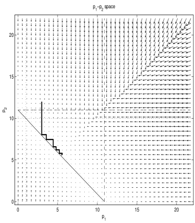
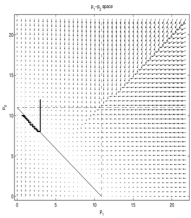
Figure 6.1: Stability of the fixed points of the differential system under one-sided positive (left-hand graph) and negative (right-hand graph) stochastic shocks.

In the price equation (5.6) in discrete time we can incorporate external random fluctuations by including a noise variable $\Delta W_{t}$:

$$\frac{\Delta p_{t}}{p_{t}}=A(t)\Delta t+\sigma\Delta W_{t}\Delta t$$

Here $\sigma>0$ is a coefficient characterizing the price variability, $\Delta W_{t}$ are independent identically distributed random variables that follow the standard Gaussian distribution. If we rewrite the above equation as

(6.1) $$\Delta p_{t}=A(t)p_{t}\Delta t+\sigma p_{t}\Delta W_{t}\Delta t,$$

under some regularity conditions, at the limit $\Delta t\rightarrow 0$, the solution of the difference equation (6.1) converges strongly to the solution of the stochastic differential equation (SDE)

(6.2) $$dp(t)=A(t)p(t)dt+\sigma p(t)dW_{t},$$

where $dW_{t}$ is the Itô stochastic differential (for more details, see [6, Theorem 9.6.2, p. 324]).

We choose a SDE of this type to govern the price dynamics in continuous time. Let us consider a 2-dimensional Wiener process $W=(W_{t},t\in[0,T])$ with components $W_{t}^{1}$ and $W_{t}^{2}$ which are independent scalar Wiener processes with respect to a common family of $\sigma$-algebras $\{\mathcal{A}_{t},t\in[0,T]\}$. According to equation (5.8) we construct the following system

$$\begin{split}dp_{t}^{1}&=Q_{1}(p_{t}^{1},p_{t}^{2})p_{t}^{1}dt+\sigma_{1}p_{t}^{1}dW_{t}^{1}\\ dp_{t}^{2}&=Q_{2}(p_{t}^{1},p_{t}^{2})p_{t}^{2}dt+\sigma_{2}p_{t}^{2}dW_{t}^{2}\end{split}$$

In a more compact form

(6.3) $$dp_{t}=a(p_{t})dt+b(p_{t})dW_{t},$$

where $p_{t}=(p_{t}^{1},p_{t}^{2})$, $a(p_{t})$ is a 2-dimensional vector function $a=(Q_{1}(.)p_{t}^{1},Q_{2}(.)p_{t}^{2})^{\prime}:\mathbb{R}^{2}\rightarrow\mathbb{R}^{2}$ and

$$b(p_{t})=\begin{pmatrix}\sigma_{1}p_{t}^{1}&0\\ 0&\sigma_{2}p_{t}^{2}\end{pmatrix}$$

is a $2\times 2$ matrix function $b(t):\mathbb{R}^{2}\rightarrow\mathbb{R}^{2\times 2}$. Some regularity conditions on $a(x)$, $b(x)$, and the initial condition $p_{t_{0}}$ should be imposed for the existence and uniqueness of a strong solution of the SDE, meaning that the solution $p_{t}$ is a measurable functional of $p_{t_{0}}$ and the Wiener process $W_{u},\ u\in[t_{0},t]$ (see Theorem 4.5.3 p. 131 and Theorem 4.5.6, p. 139 in [6]). The classical conditions given, for example, in [6] cannot be applied in our case because the function $a(x)$ violates the Lipschitz condition. There is a result due to Zvonkin which guarantees existence and uniqueness of a strong solution while imposing weaker assumptions on $a(x)$, see Theorem 6.13, p. 152 in [5]. According to it, a strong solution of the one-dimensional version of the SDE in (6.3) exists and is unique if $a(x)$ is a bounded function and $b(x)$ is Lipschitz and bounded away from zero. While we are not aware of a multi-dimensional extension of Zvonkin’s theorem, we hypothesize that a similar result holds. Under this hypothesis, a strong solution of our SDE exists and is unique.

We explore the sample paths of the solution in the phase space employing the Euler scheme to solve the stochastic differential system numerically. Figures 6.2 and 6.3 illustrate the behaviour of the stochastic differential system for different starting values of the prices. In a fashion similar to the deterministic case, the sample path approaches a stationary point depending on the initial condition. If a stationary point has been reached, the random shocks perturb the system away from it in a small neighborhood of the stationary point. The simulation studies illustrate that provided the scales $\sigma_{1}$ and $\sigma_{2}$ are small enough, the solution remains in a small neighborhood of a stationary point.

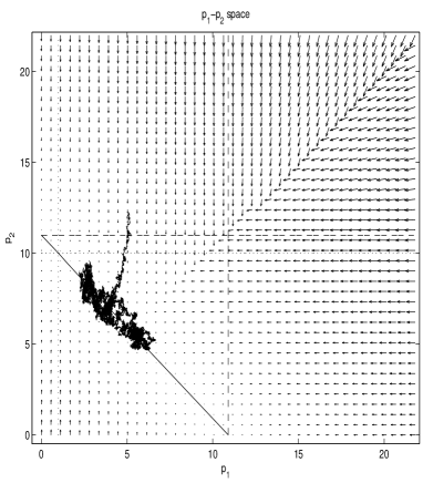
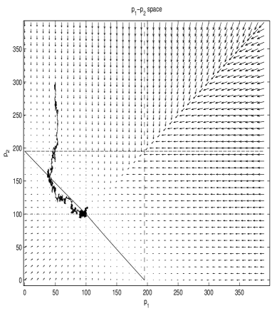
Figure 6.2: Behaviour of the differential system under stochastic shocks for different initial prices and parameterizations of the problem (1)

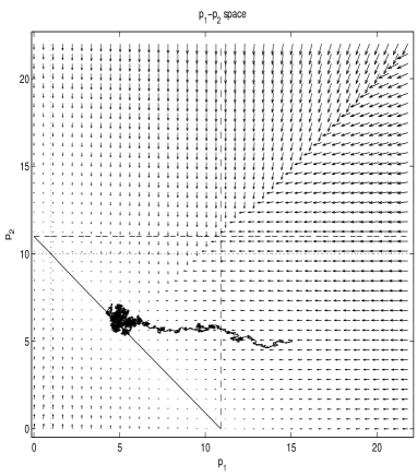
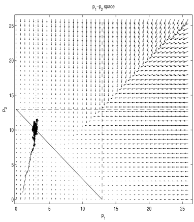
Figure 6.3: Behaviour of the differential system under stochastic shocks for different initial prices and parameterizations of the problem (2)

Appendix

Here we sketch the proofs of Propositions 4.3-4.6. Although the proof of Proposition 4.2 is contained in the main body of the paper, we will provide a sketch for it as well in order to illustrate the expository style adopted in this appendix.

We remind the reader that we always start with initial prices $p_{i,0}$. These define, through the lines $\ell_{i}$, the zone in the income space partition that the point $(Y_{1},Y_{2})$ belongs to. We also assume that $(\alpha,\beta,\gamma,\delta)$ is a NE. After determining the specific values of $(\alpha,\beta,\gamma,\delta)$, we check to what extent financial resources have been used and perform the necessary price adjustments. This leads to shifts in the lines $\ell_{i}$, thus redefining the partition and changing the position of $(Y_{1},Y_{2})$ with respect to the newly obtained zones. Ultimately, we seek to find the respective p.e.s. Whenever the use of more precise notation is called for, we write $\ell_{i,t}$, $t=0,1,2,\ldots$ The current coordinates in the equations of the respective lines are denoted by $(\tilde{Y}_{1},\tilde{Y}_{2})$.

A.1 Sketch of the proof of Proposition 4.2 for zone III

1) $q_{2}-\delta\leq 0\xrightarrow{\textrm{1-I-}A}$$\alpha=q_{1},\beta=0\xrightarrow{\textrm{2-I-}A}\gamma=0,\delta=q_{2}$. We obtain NE $\mathbf{(q_{1},0,0,q_{2})}$.

2) $0<q_{2}-\delta\leq Y_{1}/p^{\prime}_{2}\longrightarrow$ 1-II-$A_{1}$ or 1-II-$A_{2}$

- for 1-II-$A_{1}$: $\alpha=q_{1}\xrightarrow{\textrm{2-I-}A}\delta=q_{2}$ (impossible in case 2)),

- for 1-II-$A_{2}$: $q_{1}-\alpha>0$ - only for $\Delta p>\rho$ $\xrightarrow{\textrm{(3,1) 2-II-}A_{2}}$ for $\Delta p>-\rho$: $\delta=q_{2}$ (impossible).

3) $Y_{1}/p^{\prime}_{2}<q_{2}-\delta\xrightarrow{\textrm{1-III-}A}$ $q_{1}-\alpha>0$ only for $\Delta p>\rho$ $\xrightarrow{\textrm{(3,1)}}$ for $\Delta p>-\rho$: 2-II-$A_{1}~{}(A_{2})$ and 2-III-$A$ $\longrightarrow$ $q_{2}-\delta=0$, which is impossible.

For the NE $(q_{1},0,0,q_{2})$ obtained, the supply of goods is exhausted. If $Y_{i}=p_{i,0}q_{i},~{}i=1,2$, the financial resources are also exhausted, i.e. we are at a p.e. $p_{i,t}\equiv p_{i,0},~{}\forall t\geq 0,~{}i=1,2$. If for some $i$, $i=1,2$, we have $Y_{i}>p_{i,0}q_{i}$, the respective price $p_{i,0}$ is adjusted to the level $p_{i,1}$, defined by the condition $Y_{i}=p_{i,1}q_{i}$. Thus, we reach a p.e. $p_{i,t}\equiv p_{i,1},~{}\forall t\geq 1$.

A.2 Sketch of the proof of Proposition 4.3 for zone II

A.2.1 Zone II-3 (see (4.15))

1) $q_{2}-\delta\leq 0\xrightarrow{\textrm{1-I-}B}$ $\alpha=Y_{1}/p_{1}(<q_{1}),\beta=0\longrightarrow$ 1a) or 1b)

1a) $0<q_{1}-\alpha<Y_{2}/p^{\prime}_{1}\xrightarrow{\textrm{2-II-}A_{1}}$ $\gamma=q_{1}-\alpha$, $\delta=q_{2}$. We get NE $\mathbf{(Y_{1}/p_{1},0,q_{1}-Y_{1}/p_{1},q_{2})}$.

1b) $Y_{2}/p^{\prime}_{1}<q_{1}-\alpha$, which is impossible, since for $\alpha=Y_{1}/p_{1}$ we obtain that $(Y_{1},Y_{2})$ is below $\ell_{1}$ and so below $\ell_{4}$.

2) $0<q_{2}-\delta\leq Y_{1}/p^{\prime}_{2}\xrightarrow{\textrm{1-II-}B}$ $\left\{\begin{array}[]{l}\Delta p\leq\rho:~{}\alpha=Y_{1}/p_{1}(<q_{1}),~{}\beta=0\\ \Delta p>\rho:~{}\alpha=\frac{Y_{1}-p^{\prime}_{2}(q_{2}-\delta)}{p_{1}}(<q_{1}),~{}\beta=q_{2}-\delta\end{array}\right\}$ $\longrightarrow$ 2a) or 2b)

2a) $0<q_{1}-\alpha\leq Y_{2}/p^{\prime}_{1}$

- for 2-II-$A_{1}$: $\delta=q_{2}$, which is impossible in case 2).

- for 2-II-$A_{2}$: i) or ii)

i) for $\Delta p\geq-\rho$ (cases (1,1), (1,2), (2,1), (3,1)) $\longrightarrow$ $\delta=q_{2}$, which is impossible.

ii) for $\Delta p<-\rho$ (case (1,3)) $\longrightarrow$ $\delta=\frac{Y_{2}-p^{\prime}_{1}\left(q_{1}-\frac{Y_{1}}{p_{1}}\right)}{p_{2}}$ which implies, in view of the first inequality in 2), that $(Y_{1},Y_{2})$ is strictly below $\ell_{4}$.

2b) $Y_{2}/p^{\prime}_{1}<q_{1}-\alpha$ $\xrightarrow{\textrm{2-III-}A}$ i) or ii)

i) for $\Delta p\geq-\rho$: $\delta=q_{2}$ – impossible in 2)

ii) for $\Delta p<-\rho$: case (1,3), which is impossible, since inequality 2b) for $\alpha=Y_{1}/p_{1}$ implies that $(Y_{1},Y_{2})$ is below $\ell_{1}$.

3) $Y_{1}/p^{\prime}_{2}<q_{2}-\delta\xrightarrow{\textrm{1-III-}B}$ $\left\{\begin{array}[]{l}\Delta p\leq\rho:~{}\alpha=Y_{1}/p_{1},~{}\beta=0\\ \Delta p>\rho:~{}\alpha=0,~{}\beta=Y_{1}/p^{\prime}_{2}\end{array}\right\}$ $\longrightarrow$ 3a) or 3b)

3a) $0<q_{1}-\alpha\leq Y_{2}/p^{\prime}_{1}$ – impossible, see 2a)

3b) $Y_{2}/p^{\prime}_{1}<q_{1}-\alpha$ – impossible, see 2b)

For the unique NE, obtained in 1a), the quantities $q_{1}$, $q_{2}$ and $Y_{1}$ are exhausted. The condition that $(Y_{1},Y_{2})$ is above $\ell_{4}$, i.e.

(A.2.1) $$p^{\prime}_{1,0}\left(q_{1}-\frac{Y_{1}}{p_{1,0}}\right)+p_{2,0}q_{2}\leq Y_{2}$$

leads to two cases.

Case I. The condition (A.2.1) holds with equality. Then $p_{2,0}$ also remains unchanged, i.e. the points on $\ell_{4}$ in zone II are p.e.s.

Case II. If there is a strict inequality in (A.2.1), then

$$Y_{2}^{res}=Y_{2}-p^{\prime}_{1,0}\left(q_{1}-\frac{Y_{1}}{p_{1,0}}\right)>p_{2,0}q_{2}.$$

We increase $p_{2,0}$ to $p_{2,1}$, for which $p_{2,1}q_{2}=Y_{2}^{res}$. With the new prices $p_{1,1}=p_{1,0}$ and $p_{2,1}$, the point $(Y_{1},Y_{2})$ falls on the line

$$\ell_{4,1}:p_{2,1}q_{2}+p^{\prime}_{1,0}q_{1}=\tilde{Y}_{2}+\frac{p^{\prime}_{1,0}}{p_{1,0}}\tilde{Y}_{1},$$

i.e. the p.e. is reached in one adjustment step.

A.2.2 Zone II-2 (see (4.14))

1) $q_{2}-\delta\leq 0\xrightarrow{\textrm{1-I-}B}$ $\alpha=Y_{1}/p_{1}(<q_{1}),\beta=0\longrightarrow$ 1a) or 1b)

1a) $0<q_{1}-\alpha\leq Y_{2}/p^{\prime}_{1}$

- case 2-II-$A_{1}$ is impossible, since $(Y_{1},Y_{2})$ is below $\ell_{4}$

- case 2-II-$A_{2}$ $\longrightarrow$ i) or ii)

i) for $\Delta p\geq-\rho$: $\gamma=\frac{Y_{2}-p_{2}q_{2}}{p^{\prime}_{1}},~{}\delta=q_{2}$, which leads for $\boldsymbol{\Delta p\geq-\rho}$ to

$$\textrm{{NE}}\mathbf{\left(\frac{Y_{1}}{p_{1}},0,\frac{Y_{2}-p_{2}q_{2}}{p^{\prime}_{1}},q_{2}\right).}$$

ii) for $\Delta p<-\rho$ $\longrightarrow$ $\delta<q_{2}$, which is impossible in 1).

1b) $q_{1}-\alpha>Y_{2}/p^{\prime}_{1}$, which is impossible for $\alpha=Y_{1}/p_{1}$.

2) $0<q_{2}-\delta\leq Y_{1}/p^{\prime}_{2}\xrightarrow{\textrm{1-II-}B}$ $\left\{\begin{array}[]{l}\Delta p\leq\rho:~{}\alpha=Y_{1}/p_{1}(<q_{1}),\beta=0\\ \Delta p>\rho:\alpha=\frac{Y_{1}-p^{\prime}_{2}(q_{2}-\delta)}{p_{1}}(<q_{1}),\beta=q_{2}-\delta\end{array}\right\}$ $\longrightarrow$ 2a) or 2b)

2a) $0<q_{1}-\alpha\leq Y_{2}/p^{\prime}_{1}$

- case 2-II-$A_{1}$: $\delta=q_{2}$, which is impossible in 2)

- case 2-II-$A_{2}$ $\longrightarrow$ i) or ii)

i) for $\Delta p\geq-\rho$ $\longrightarrow$ $\delta=q_{2}$, which is impossible in 2)

ii) for $\boldsymbol{\Delta p<-\rho}$: only (1,3) $\longrightarrow$ We have

$$\textrm{{NE}}\mathbf{\left(\frac{Y_{1}}{p_{1}},0,q_{1}-\frac{Y_{1}}{p_{1}},\frac{Y_{2}-p^{\prime}_{1}(q_{1}-Y_{1}/p_{1})}{p_{2}}\right)}.$$

(In this case the condition $\delta<q_{2}$ is obviously satisfied. A comment on the second condition, $q_{2}-\delta\leq Y_{2}/p^{\prime}_{1}$, is offered following case 3a).)

2b) $Y_{2}/p^{\prime}_{1}<q_{1}-\alpha$ $\longrightarrow$ i) or ii)

i) for $\alpha=Y_{1}/p_{1}$ (i.e. for $\Delta p\leq\rho$): $(Y_{1},Y_{2})$ is strictly below $\ell_{1}$, which is impossible.

ii) for $\Delta p>\rho$: only (3,1) $\xrightarrow{\textrm{2-III-}A}$ $\delta=q_{2}$, which is impossible in 2).

3) $Y_{1}/p^{\prime}_{2}<q_{2}-\delta$ $\xrightarrow{\textrm{1-III-}B}$ $\left\{\begin{array}[]{l}\Delta p\leq\rho:~{}\alpha=Y_{1}/p_{1}(<q_{1}),~{}\beta=0\\ \Delta p>\rho:~{}\alpha=0(<q_{1}),~{}\beta=Y_{1}/p^{\prime}_{2}\end{array}\right\}$ $\longrightarrow$ 3a) or 3b)

3a) $0<q_{1}-\alpha\leq Y_{2}/p^{\prime}_{1}$ $\longrightarrow$ i) or ii)

i) for 2-II-$A_{1}$: $\delta=q_{2}$ – impossible in 3)

ii) for 2-II-$A_{2}$ $\longrightarrow$ $\Delta p\geq-\rho$ or $\Delta p<-\rho$

- for $\Delta p\geq-\rho$: $\delta=q_{2}$ – impossible

- for $\Delta p<-\rho$: only (1,3) $\longrightarrow$ $\gamma=q_{1}-Y_{1}/p_{1},~{}\delta=\frac{Y_{2}-p^{\prime}_{1}(q_{1}-Y_{1}/p_{1})}{p_{2}}$, which leads to the same NE as in case 2a)-(1,3).
(It turns out that whether $q_{2}-\delta$ is greater than or less than $Y_{1}/p^{\prime}_{2}$ is irrelevant, since we obtain the same NE.)

3b) $Y_{2}/p^{\prime}_{1}<q_{1}-\alpha$ $\xrightarrow{\textrm{2-III-}A}$ case $\Delta p\geq-\rho$ or case $\Delta p<-\rho$

- case $\Delta p\geq-\rho$: $\delta=q_{2}$ – impossible

- case $\Delta p<-\rho$: only (1,3) $\longrightarrow$ condition 3b) would imply that $(Y_{1},Y_{2})$ is below $\ell_{1}$, which is impossible.

We now turn to the study of the price dynamics, starting from the NE obtained above.

I) Analysis of the case NE $\mathbf{\left(\frac{Y_{1}}{p_{1,0}},0,q_{1}-\frac{Y_{1}}{p_{1,0}},\frac{Y_{2}-p^{\prime}_{1,0}(q_{1}-Y_{1}/p_{1,0})}{p_{2,0}}\right)}$ (see 2a) or 3a) for $\boldsymbol{\Delta p<-\rho}$)

The quantities $Y_{1}$, $q_{1}$ and $Y_{2}$ are depleted. Since $(Y_{1},Y_{2})$ is strictly below $\ell_{4}$, we have $\delta<q_{2}$, i.e. $q_{2}$ is not used up completely. Additionally,

(A.2.2) $$q_{2,0}^{cons}=\delta=\frac{1}{p_{2,0}}\left[Y_{2}+\frac{p^{\prime}_{1,0}}{p_{1,0}}Y_{1}-p^{\prime}_{1,0}q_{1}\right]\geq 0,$$

since $(Y_{1},Y_{2})$ is on or above $\ell_{1}$.

Case I,i): In (A.2.2) we have $q_{2,0}^{cons}>0$, i.e. $(Y_{1},Y_{2})$ is strictly above $\ell_{1}$. Now $p_{2,0}$ decreases to $p_{2,1}$, which is defined by

$$p_{2,1}q_{2}=p_{2,0}q_{2,0}^{cons}=Y_{2}-p^{\prime}_{1,0}\left(q_{1}-\frac{Y_{1}}{p_{1,0}}\right).$$

Since $p_{1,1}=p_{1,0}$, the point $(Y_{1},Y_{2})$ turns out to be on the line $\ell_{4,1}$, which is parallel to $\ell_{4,0}$, whose points are all equilibria, i.e. we reach a p.e. in one adjustment step.

The above case is graphically illustrated in Figure A.1.

Figure A.1: Price adjustment in case I,i).

Case I,ii): In (A.2.2) we have $q_{2,0}^{cons}=0$, which is possible for the points in $\ell_{1,0}\bigcap\{\textrm{Zone II}\}$, where $q_{1}-Y_{1}/p_{1,0}=Y_{2}/p^{\prime}_{1,0}$. Consequently, $p_{2,0}$ is reduced to $p_{2,1}=0$ (while $p_{1,1}=p_{1,0}$) and we reach a degenerate case. Writing for brevity $(p_{1},0)$ instead of $(p_{1,1},p_{2,1})$, this case is described by Table 3.1 for $p^{\prime}_{2}=\rho,p_{1}>0$, and Table 3.4. We now have the problem of finding NE $(\alpha,\beta,\gamma,\delta)$ subject to the constraints

(A.2.3) $$0<Y_{1}<p_{1}q_{1},0<Y_{2}$$

and the additional condition

(A.2.4) $$\frac{Y_{1}}{p_{1}}+\frac{Y_{2}}{p^{\prime}_{1}}=q_{1}.$$

We solve the problem through the already familiar approach:

1) $q_{2}-\delta\leq 0$ $\xrightarrow{\textrm{1-I-}B}$ $\alpha=Y_{1}/p_{1}(<q_{1}),~{}\beta=0$ $\longrightarrow$ 1a) or 1b)

1a) $0<q_{1}-\alpha=Y_{2}/p^{\prime}_{1}$ $\xrightarrow{\textrm{4-II}}$ $\gamma=q_{1}-\alpha,~{}\delta=q_{2}$.

This leads to NE $\mathbf{\left(\frac{Y_{1}}{p_{1}},0,q_{1}-\frac{Y_{1}}{p_{1}},q_{2}\right)}=\mathbf{\left(\frac{Y_{1}}{p_{1,0}},0,\frac{Y_{2}}{p^{\prime}_{1,0}},q_{2}\right)}$

Since all resources are depleted, we reach a degenerate p.e., for which

$$p_{1,t}=p_{1,0},~{}p_{2,t}=0,~{}\forall t\geq 1.$$

Obviously only the first economy is fully functioning, while in the second economy local output becomes irrelevant as its market price is zero.

1b) $Y_{2}/p^{\prime}_{1}<q_{1}-\alpha$, which is impossible since $(Y_{1},Y_{2})$ is above $\ell_{1}$.

In the degenerate case there are no other NE, since for all possible cases, namely

2) $0<q_{2}-\delta\leq Y_{1}/\rho$
or

3) $Y_{1}/\rho<q_{2}-\delta$,
after applying Table 3.4, we obtain $\delta=q_{2}$, which leads to a contradiction.

This completes the analysis of case I).

II) Analysis of the case NE $\mathbf{\left(\frac{Y_{1}}{p_{1,0}},0,\frac{Y_{2}-p_{2,0}q_{2}}{p^{\prime}_{1,0}},q_{2}\right)}$ (see 1a) for $\boldsymbol{\Delta p\geq-\rho}$)

The quantities $Y_{1}$, $Y_{2}$ and $q_{2}$ are depleted and the condition that $(Y_{1},Y_{2})$ is below $\ell_{4}$ is equivalent to

$$q_{1}>\left[\frac{Y_{1}}{p_{1,0}}+\frac{1}{p^{\prime}_{1,0}}\left(Y_{2}-p_{2,0}q_{2}\right)\right]=q_{1,0}^{cons},$$

i.e. $q_{1}$ is not depleted. At the same time,

$$q_{1,0}^{cons}=\frac{Y_{1}}{p_{1,0}}+\frac{Y_{2}}{p^{\prime}_{1,0}}-\frac{p_{2,0}q_{2}}{p^{\prime}_{1,0}}\geq q_{1}-\frac{p_{2,0}q_{2}}{p^{\prime}_{1,0}}=\frac{\rho q_{1}+p_{1,0}q_{1}-p_{2,0}q_{2}}{p^{\prime}_{1,0}}>0$$

according to (4.1). Consequently, $p_{1,0}$ is reduced to $p_{1,1}$, where

(A.2.5) $$p_{1,1}q_{1}=p_{1,0}q_{1,0}^{cons}=Y_{1}+\frac{p_{1,0}}{p^{\prime}_{1,0}}\left(Y_{2}-p_{2,0}q_{2}\right).$$

The following subcases are possible:

II,i) $Y_{2}=p_{2,0}q_{2}$, i.e. $(Y_{1},Y_{2})$ is a point on the segment $FE_{0}$ in Figure A.1. Now the NE under consideration takes the form $(Y_{1}/p_{1},0,0,q_{2})$. After the above adjustment of $p_{1,0}$, $(Y_{1},Y_{2})$ turns out to be at $E_{1}$, i.e. we reach a p.e. for which

$$p_{1,t}=p_{1,1},~{}p_{2,t}=p_{2,0},~{}\forall t\geq 1.$$

II,ii) $Y_{2}>p_{2,0}q_{2}$. First we find the location of $(Y_{1},Y_{2})$ with respect to the new position of $\ell_{4,0}$ (after the adjustment (A.2.5)) i.e. with respect to

$$\ell_{4,1}:p_{2,0}q_{2}+p^{\prime}_{1,1}q_{1}=\frac{p^{\prime}_{1,1}}{p_{1,1}}\tilde{Y}_{1}+\tilde{Y}_{2}.$$

We compare $p_{2,0}q_{2}-Y_{2}$ and

$$\frac{p^{\prime}_{1,1}}{p_{1,1}}\left(Y_{1}-p_{1,1}q_{1}\right)=\frac{p^{\prime}_{1,1}}{p_{1,1}}\left[Y_{1}-Y_{1}-\frac{p_{1,0}}{p^{\prime}_{1,0}}\left(Y_{2}-p_{2,0}q_{2}\right)\right]=\left(p_{2,0}q_{2}-Y_{2}\right)\frac{p^{\prime}_{1,1}}{p_{1,1}}\frac{p_{1,0}}{p^{\prime}_{1,0}}.$$

Since $p_{1,1}=p_{1,0}-\Delta$, $\Delta>0$, it is easy to check that

$$\frac{p^{\prime}_{1,1}}{p_{1,1}}\frac{p_{1,0}}{p^{\prime}_{1,0}}>1,$$

which, after multiplication by $p_{2,0}q_{2}-Y_{2}(<0)$, yields

$$p_{2,0}q_{2}-Y_{2}>\frac{p^{\prime}_{1,1}}{p_{1,1}}(Y_{1}-p_{1,1}q_{1}).$$

Consequently, $(Y_{1},Y_{2})$ turns out to be below $\ell_{4,1}$.

The results obtained are illustrated graphically in Figure A.2. Let $\tilde{\ell}$ denote a line through the point $(Y_{1},Y_{2})$, which is parallel to $\ell_{4,0}$, i.e.

$$\tilde{\ell}:\frac{p^{\prime}_{1,0}}{p_{1,0}}\tilde{Y}_{1}+\tilde{Y}_{2}=const\left(=\frac{p^{\prime}_{1,0}Y_{1}}{p_{1,0}}+Y_{2}\right).$$

Obviously, the point M$(p_{1,1}q_{1},p_{2,0}q_{2})$ lies on $\tilde{\ell}$, as well as on $\ell_{4,1}$. Also, since

$$\tan\theta_{0}=\frac{p^{\prime}_{1,0}}{p_{1,0}}<\frac{p^{\prime}_{1,1}}{p_{1,1}}=\tan\theta_{1},$$

it follows that

$$\theta_{0}<\theta_{1}.$$

Thus, the line $\ell_{4,1}$ must turn in the negative direction around the point M to coincide with $\tilde{\ell}$. Since $(Y_{1},Y_{2})$ lies on $\tilde{\ell}$, it is located below $\ell_{4,1}$. At the same time, as $\ell_{1,1}$ is below $\ell_{1,0}$, the point $(Y_{1},Y_{2})$ remains above $\ell_{1,1}$.

Figure A.2: Price adjustment in case II,ii)

Obviously, $p^{\prime}_{1,1}<p^{\prime}_{1,0}$ and $p_{2,0}q_{2}<p^{\prime}_{1,0}q_{1}$, yet it is possible for $p^{\prime}_{1,1}q_{1}$ to be greater or smaller than $p_{2,0}q_{2}$ (see below).

We shall study separately the cases

II,ii-1) $\Delta p=-\rho$, i.e. $p^{\prime}_{1,0}=p_{2,0}$,

II,ii-2) $\Delta p>-\rho$, i.e. $p^{\prime}_{1,0}>p_{2,0}$.

In case II,ii-1), after a downward adjustment of $p_{1,0}$ to $p_{1,1}$ (see (A.2.5)) we obtain (in the new zone II-2 – see Figure A.2, between $\ell_{4,1}$ and $\ell_{1,1}$) the case leading to NE for $\Delta p<-\rho$ of the type in case I,i). Consequently, after an adjustment of $p_{2,1}=p_{2,0}$ to a smaller positive value $p_{2,2}$, the point $(Y_{1},Y_{2})$ lies on $\ell_{4,2}$, whose points are equilibria. Note also that even if $(Y_{1},Y_{2})\in\ell_{1,0}$, this point will be strictly above $\ell_{1,1}$ and so a degenerate equilibrium cannot be obtained.

In case II,ii-2) there are many possibilities, which we describe below. Suppose that, after the first adjustment of $p_{1,0}$ as per (A.2.5) down to $p_{1,1}$, we obtain the condition $\Delta p\leq-\rho$, i.e. $p^{\prime}_{1,1}\leq p_{2,1}$. (We have $p_{2,1}=p_{2,0}$, since only $p_{1,0}$ has been changed.) Then, when consumption in the next period is carried out ($t=2$), the above described adjustment according to the NE of type I,i) obtains.

To find out whether such points exist at all, we write the condition (which is the converse of the one mentioned above)

(A.2.6) $$p^{\prime}_{1,1}>p_{2,0}$$

in the equivalent form

(A.2.7) $$Y_{1}+\frac{p_{1,0}}{p^{\prime}_{1,0}}Y_{2}>(p_{2,0}-\rho)q_{1}+\frac{p_{1,0}}{p^{\prime}_{1,0}}p_{2,0}q_{2}.$$

Consequently, the condition (A.2.6) means that the point $(Y_{1},Y_{2})$ is above the line

$$\bar{\bar{\ell}}:\tilde{Y}_{1}+\frac{p_{1,0}}{p^{\prime}_{1,0}}\tilde{Y}_{2}=(p_{2,0}-\rho)q_{1}+\frac{p_{1,0}}{p^{\prime}_{1,0}}p_{2,0}q_{2},$$

which is parallel to $\ell_{4,0}$ and $\ell_{1,0}$. Since the abscissa of the intersection point of $\bar{\bar{\ell}}$ with the $\tilde{Y}_{1}$ axis is smaller than the abscissa of the intersection point of $\ell_{4,0}$ (in view of II,ii-2)), there exist points $(Y_{1},Y_{2})$ in zone II-2 with the property (A.2.6). Respectively, in the case when (A.2.6) does not hold, the relevant points belong to the closed area in zone II-2 enclosed between $\ell_{1,0}$ and $\bar{\bar{\ell}}$ (when $\bar{\bar{\ell}}$ is between $\ell_{1,0}$ and $\ell_{4,0}$), or the segment of $\ell_{1,0}=\bar{\bar{\ell}}$ belonging to zone II-2 (when the last two line coincide), and for then the adjustment process from II,ii-1) obtains. When $\bar{\bar{\ell}}$ is strictly below $\ell_{1,0}$, no such points exist.

For all points strictly above $\bar{\bar{\ell}}$ the conditions

$$p^{\prime}_{1,0}>p_{2,0}\textrm{ and }p^{\prime}_{1,1}>p_{2,0}$$

are simultaneously valid.

Figure A.3 illustrates this case, with $\bar{\bar{\ell}}$ taken to lie between $\ell_{1,0}$ and $\ell_{4,0}$ for determinacy.

Figure A.3: Price adjustment in case II,ii-2)

In the new zone II-2, defined by $\ell_{1,1}$ and $\ell_{4,1}$, we again obtain a NE of type II. However, because of the rotation at an angle $\theta_{1}-\theta_{0}$ in the negative direction (see above), it is not certain whether after the adjustment in $p_{1,1}$ (in which a reduction to $p_{1,2}$ occurs), we can have

(A.2.8) $$p^{\prime}_{1,2}>p_{2,2}~{}(=p_{2,0}),$$

i.e. whether $(Y_{1},Y_{2})$ would be above $\bar{\bar{\ell}}_{new}$ (see Figure A.3).

To describe all possible cases, we introduce the function

(A.2.9) $$g(x)=\frac{1}{q_{1}}\left[Y_{1}+\left(Y_{2}-p_{2,0}q_{2}\right)\frac{x}{x+\rho}\right],$$

for which $g(0)>0$, $g^{\prime}(x)>0$, $\lim_{x\rightarrow\infty}g(x)>g(0)>0$ (see Figure A.4).

Figure A.4: The function $g(x)$

With the aid of the function $g(x)$, the condition that the point $(Y_{1},Y_{2})$ is below the line $\ell_{4,0}$ becomes equivalent to

(A.2.10) $$p_{1,0}>g(p_{1,0}).$$

This, in particular, implies that $p_{1,0}>k$, where $k$ is the only positive number defined by $k=g(k)$.

Respectively, the condition (A.2.5) determining $p_{1,1}$ can be written as

(A.2.11) $$p_{1,1}=g(p_{1,0}).$$

If (A.2.8) were valid, in the next step we would set

$$p_{1,2}=g(p_{1,1})=g^{2}(p_{1,0})$$

and so on.

There are two possible cases:

II,ii-2a): $p_{2,0}-\rho\leq k(<p_{1,0})$,

II,ii-2b): $k<p_{2,0}-\rho~{}(<p_{1,0})$.

Case II,ii-2a). In this case

$$p_{1,1}=g(p_{1,0})>g(k)=k\geq p_{2}-\rho.$$

We reach a NE of the type II,ii) and set

$$p_{1,2}=g(p_{1,1})>k\geq p_{2}-\rho$$

etc.

$$p_{1,t+1}=g(p_{1,t}),~{}\forall t>0.$$

Obviously the sequence $\{p_{1,t}\}$ is convergent and tends to $k$. The points S, T and M in Figure A.3 have abscissas respectively $(p_{2,0}-\rho)q_{1}$, $kq_{1}$ and $p_{1,1}q_{1}$, and the line through T and $(Y_{1},Y_{2})$ is the limit position of $\ell_{4}$ after infinitely many adjustments of the first price.

Case II,ii-2b). Let

$$p_{2,0}-\rho\in[g^{s}(p_{1,0}),g^{s-1}(p_{1,0)}],$$

where $s$ is a natural number. In this case, after $s$ adjustments of the first price, we reach an equilibrium for which the respective NE is of type I) and the price adjustment process evolves accordingly.

Remark A.2.1.

It is possible, as a result of the price reduction in the first market, to reach for some $t\in\mathbb{N}$ the situation

$$p^{\prime}_{1,t}\leq p_{2,0}q_{2},$$

i.e. zone II-1 disappears. (As a matter of fact, this is the case of zone IV-2, with the roles of the two economies reversed.) We can directly see that if $p^{\prime}_{1,0}q_{1}\leq p_{2,0}q_{2}$, in the ‘‘expanded’’ zone II-2

$$\left\{\begin{array}[]{l}Y_{1}<p_{1}q_{1},~{}Y_{2}\geq p_{2}q_{2}\\ (Y_{1},Y_{2})\textrm{ is stricly below }\ell_{4}\end{array}\right.$$

one obtains the NEs of type I) and II) derived above. The only qualitative difference here is that no degenerate equilibria exist. $\blacksquare$

A.2.3 Zone II-1 (see (4.13))

We note that this zone is characterized by relatively low financial resources in both economies. We have $Y_{1}<Y_{0}$, where the point $(Y_{0},p_{2}q_{2})=\ell_{1}\bigcap\{\tilde{Y}_{2}=p_{2}q_{2}\}$ and $Y_{2}<p^{\prime}_{1}q_{1}$. To find the NE one proceeds as follows.

1) $q_{2}-\delta\leq 0\xrightarrow{\textrm{1-I-}B}$ $\alpha=Y_{1}/p_{1}(<q_{1}),\beta=0\longrightarrow$ 1a) or 1b)

1a) $0<q_{1}-\alpha\leq Y_{2}/p^{\prime}_{1}$ is impossible, since for $\alpha=Y_{1}/p_{1}$ the point $(Y_{1},Y_{2})$ would be above $\ell_{1}$.

1b) $Y_{2}/p^{\prime}_{1}<q_{1}-\alpha$ $\xrightarrow{\textrm{2-III-}A}$ i) or ii)

i) for $\boldsymbol{\Delta p\geq-\rho}$: $\gamma=\frac{Y_{2}-p_{2}q_{2}}{p^{\prime}_{1}},\delta=q_{2}$, which leads to the NE $\mathbf{\left(\frac{Y_{1}}{p_{1}},0,\frac{Y_{2}-p_{1}q_{2}}{p^{\prime}_{1}},q_{2}\right)}$.

ii) for $\Delta p<-\rho\longrightarrow$ $\delta=0\longrightarrow q_{2}-\delta>0$, which is impossible in 1).

2) $0<q_{2}-\delta\leq Y_{1}/p^{\prime}_{2}$ $\xrightarrow{\textrm{1-III-}B}$ $\left\{\begin{array}[]{l}\Delta p\leq\rho:~{}\alpha=\frac{Y_{1}}{p_{1}}(<q_{1}),~{}\beta=0\\ \Delta p>\rho:~{}\alpha=\frac{Y_{1}-p^{\prime}_{2}(q_{2}-\delta)}{p_{1}}(<q_{1}),~{}\beta=q_{2}-\delta\end{array}\right\}$ $\longrightarrow$ 2a) or 2b)

2a) $0<q_{1}-\alpha\leq Y_{2}/p^{\prime}_{1}$

- for $\Delta p\leq\rho$: impossible (see 1a))

- for $\Delta p>\rho$: only (3,1) $\longrightarrow$ 2-II-$A_{1}$ and 2-II-$A_{2}$ ($\Delta p>-\rho$) $\longrightarrow$ $\delta=q_{2}$ – impossible.

2b) $q_{1}-\alpha>Y_{2}/p^{\prime}_{1}$ $\xrightarrow{\textrm{2-III-}A}$ case $\Delta p\geq-\rho$ or case $\Delta p<-\rho$

- for $\Delta p\geq-\rho$: $\delta=q_{2}$ – impossible.

- for $\boldsymbol{\Delta p<-\rho}$: only in (1,3), $\gamma=Y_{2}/p^{\prime}_{1},\delta=0$, which leads to the NE $\mathbf{\left(\frac{Y_{1}}{p_{1}},0,\frac{Y_{2}}{p^{\prime}_{1}},0\right)}$. (See the comment after 3b) for a check of the condition $q_{2}-0\leq Y_{1}/p^{\prime}_{2}$.)

3) $Y_{1}/p^{\prime}_{2}<q_{2}-\delta$ $\xrightarrow{\textrm{1-III-}B}$ $\left\{\begin{array}[]{l}\Delta p\leq\rho:~{}\alpha=Y_{1}/p_{1}(<q_{1}),~{}\beta=0\\ \Delta p>\rho:~{}\alpha=0(<q_{1}),~{}\beta=Y_{2}/p^{\prime}_{2}\end{array}\right\}$ $\longrightarrow$ 3a) or 3b)

3a) $0<q_{1}-\alpha\leq Y_{2}/p^{\prime}_{1}$

- for $\Delta p\leq\rho$ – impossible (see 1a))

- for $\Delta p>\rho$ – impossible (see 1a))

3b) $q_{1}-\alpha>Y_{2}/p^{\prime}_{1}$ $\xrightarrow{\textrm{2-III-}A}$ case $\Delta p\geq-\rho$ or case $\Delta p<-\rho$

- for $\Delta p\geq-\rho$: $\delta=q_{2}$ – impossible

- for $\Delta p<-\rho$: only in (1,3), $\gamma=Y_{2}/p^{\prime}_{1},\delta=0$, which leads to the same NE as in 2b). (It follows that the check whether $Y_{1}/p^{\prime}_{2}$ is less than or greater than $q_{2}$ is unnecessary.)

We now turn to the study of the price dynamics, starting from the NE obtained above.

I) Analysis of the case NE $\mathbf{\left(\frac{Y_{1}}{p_{1,0}},0,\frac{Y_{2}}{p^{\prime}_{1,0}},0\right)}$ for $\boldsymbol{\Delta p<-\rho}$ (see 2a) or 3b))

The financial resources $Y_{i}$ are depleted, $q_{1}$ is only consumed in part (since $(Y_{1},Y_{2})$ is strictly below $\ell_{1}$ and thus $q_{1,0}^{cons}\in(0,q_{1})$) and $q_{2}$ is unchanged ($q_{2,0}^{cons}=0$). Consequently, $p_{2,1}=0$ and $p_{1,1}<p_{1,0}$ is determined by

$$p_{1,1}q_{1}=p_{1,0}q_{1,0}^{cons}=Y_{1}+\frac{p_{1,0}}{p^{\prime}_{1,0}}Y_{2}.$$

It is immediately seen that the point $(Y_{1},Y_{2})$ remains below the line

$$\ell_{1,1}:p_{1,1}q_{1}=\tilde{Y}_{1}+p_{1,1}\frac{\tilde{Y}_{2}}{p^{\prime}_{1,1}}$$

and (omitting the index $t=1$) this point lies in the following set (degenerate zone II-1):

(A.2.12) $$\left\{\begin{array}[]{l}\frac{Y_{1}}{p_{1}}+\frac{Y_{2}}{p^{\prime}_{1}}<q_{1},\\ 0<Y_{1}<p_{1}q_{1},~{}0<Y_{2}.\end{array}\right.$$

Figure A.5 provides a geometric illustration of the adjustment of the line $\ell_{1}$ in the case when the price $p_{1}$ is reduced.

Figure A.5: The adjustment of the line $\ell_{1}$ when $p_{1}$ is reduced

The line $\tilde{\ell}$, passing through the point $(Y_{1},Y_{2})$, is parallel to $\ell_{1,0}$ and has the equation

$$\tilde{\ell}:\tilde{Y}_{1}+\frac{p_{1,0}}{p^{\prime}_{1,0}}\tilde{Y}_{2}=Y_{1}+\frac{p_{1,0}}{p^{\prime}_{1,0}}Y_{2}=p_{1,1}q_{1}.$$

It intersects the line

$$\ell_{1,1}:\tilde{Y}_{1}+\frac{p_{1,1}}{p^{\prime}_{1,1}}\tilde{Y}_{2}=p_{1,1}q_{1}$$

at the point $K(p_{1,1}q_{1})$. Since (see Figure A.5 for the notation)

$$\tan\theta_{1}=\frac{p^{\prime}_{1,0}}{p_{1,0}}<\frac{p^{\prime}_{1,1}}{p_{1,1}}=\tan\theta_{2}\Rightarrow\theta_{1}<\theta_{2},$$

it is obvious that $(Y_{1},Y_{2})$ is below $\ell_{1,1}$.

Using Table 3.1 (for $p^{\prime}_{2}=\rho$ and $p_{1}>0$) and Table 3.4, we find the NE $\mathbf{\left(\frac{Y_{1}}{p_{1,0}},0,\frac{Y_{2}}{p^{\prime}_{1,0}},0\right)}$ for the set defined in (A.2.12). For this NE, $Y_{1}$, $Y_{2}$ and $q_{2}$ are depleted, so the price $p_{1}~{}(=p_{1,1})$ is reduced, as above, to $p_{1,2}=h(p_{1,1})\equiv\frac{1}{q_{1}}\left[Y_{1}+\frac{p_{1,1}}{p_{1,1}+\rho}Y_{2}\right]$.

This adjustment process for the price is infinite and in the limit we reach

$$p_{1,\infty}=\lim_{t\rightarrow\infty}p_{1,t},$$

where $p_{1,\infty}$ is the positive solution of the equation $k=h(k)$. In general, the prices tend to (although they never reach it) a degenerate ‘‘equilibrium’’

$$p_{1,t}\rightarrow p_{1,\infty},~{}p_{2,t}=0,~{}\forall t\geq 0.$$

In this situation, the limiting position of $(Y_{1},Y_{2})$ is on the line

(A.2.13) $$\ell_{1,\infty}:\frac{\tilde{Y}_{1}}{p_{1,\infty}}+\frac{\tilde{Y}_{2}}{p^{\prime}_{1,\infty}}=q_{1}.$$

From this one can easily obtain the number

(A.2.14) $$p_{1,\infty}=\frac{1}{2q_{1}}\left(Y_{1}+Y_{2}-\rho q_{1}+\sqrt{(Y_{1}+Y_{2}-\rho q_{1})^{2}+4\rho q_{1}Y_{1}}\right).$$

Returning to the situation shown in Figure A.5, we note that in the adjustment process for $p_{1}$ described above, the points $(p_{1,t}q_{1},0)$, which are counterparts to the point $K$, tend to the limit point $(p_{1,\infty}q_{1},0)$, while the lines $\ell_{1,t}$ converge to the limit position $\ell_{1,\infty}$ (with the latter line passing through $(Y_{1},Y_{2})$).

II) Analysis of the case NE $\mathbf{\left(\frac{Y_{1}}{p_{1,0}},0,\frac{Y_{2}-p_{2,0}q_{2}}{p^{\prime}_{1,0}},q_{2}\right)}$ for $\boldsymbol{\Delta p\geq-\rho}$ (see 1b))

The analysis and results in this case coincide with those for case II) from b) from Proposition 4.3 (when the constraint coming from $\ell_{1}$ is not binding).

A.3 Sketch of the proof of Proposition 4.4 for zone I

The financial resources are smaller than the supply in both economies, which technically means that we shall use parts $B$ in Tables 3.1 and 3.2. For the same reason, the relationship between initial prices and transportation costs plays an important role for the evolution of prices here.

A.3.1 Zone I-1 (see (4.17))

1) $q_{2}-\delta\leq 0$ $\xrightarrow{\textrm{1-I-}B}$ $\alpha=Y_{1}/p_{1}(<q_{1}),\beta=0$ $\longrightarrow$ 1a) or 1b)

1a) $0<q_{1}-\alpha\leq Y_{2}/p^{\prime}_{1}$ $\xrightarrow{\textrm{2-II-}B}$ $q_{2}-\delta\geq q_{2}-Y_{2}/p_{2}>0$, which is impossible in 1).

1b) $Y_{2}/p^{\prime}_{1}<q_{1}-\alpha$ – impossible for $\alpha=Y_{1}/p_{1}$, since it would imply that $(Y_{1},Y_{2})$ is strictly below $\ell_{1}$.

2) $0<q_{2}-\delta\leq Y_{2}/p^{\prime}_{2}$ $\xrightarrow{\textrm{1-II-}B}$ $\left\{\begin{array}[]{l}\Delta p\leq\rho:~{}\alpha=Y_{1}/p_{1}(<q_{1}),~{}\beta=0\\ \Delta p>\rho:~{}\alpha=\frac{Y_{1}-p^{\prime}_{2}(q_{2}-\delta)}{p_{1}}(<q_{1}),~{}\beta=q_{2}-\delta\end{array}\right\}$ $\longrightarrow$ 2a) or 2b)

2a) $0<q_{1}-\alpha\leq Y_{2}/p^{\prime}_{1}$ $\xrightarrow{\textrm{2-II-}B}$ i) or ii)

i) for $\Delta p\geq-\rho$: $\gamma=0,\delta=Y_{2}/p_{2}$

ii) for $\Delta p<-\rho$: $\gamma=q_{1}-\alpha,\delta=\frac{Y_{2}-p^{\prime}_{1}(q_{1}-\alpha)}{p_{2}}$

We obtain respectively:

- in cases (1,1), (1,2) and (2,1), i.e. for $\boldsymbol{\Delta p\in[-\rho,\rho]}$: NE $\mathbf{\left(\frac{Y_{1}}{p_{1}},0,0,\frac{Y_{2}}{p_{2}}\right)}$

- in case (1,3), $\boldsymbol{\Delta p<-\rho}$: NE $\mathbf{\left(\frac{Y_{1}}{p_{1}},0,q_{1}-\frac{Y_{1}}{p_{1}},\frac{Y_{2}-p^{\prime}_{1}\left(q_{1}-\frac{Y_{1}}{p_{1}}\right)}{p_{2}}\right)}$

- in case (3,1), $\boldsymbol{\Delta p>\rho}$: NE $\mathbf{\left(\frac{Y_{1}-p^{\prime}_{2}\left(q_{2}-\frac{Y_{2}}{p_{2}}\right)}{p_{1}},q_{2}-\frac{Y_{2}}{p_{2}},0,\frac{Y_{2}}{p_{2}}\right)}$.

(The condition from 2) holds for $\delta=Y_{2}/p_{2}$, since $(Y_{1},Y_{2})$ is above $\ell_{2}$. For a check of the condition when $\delta$ is as in the NE for $\Delta p<-\rho$, see 3a). The condition $q_{1}\leq\alpha-Y_{2}/p^{\prime}_{1}$ holds for $\alpha=Y_{1}/p_{1}$, since $(Y_{1},Y_{2})$ is above $\ell_{1}$. For a check of the condition when $\alpha$ is as in the NE for $\Delta p>\rho$, see 2b).)

2b) $Y_{2}/p^{\prime}_{1}<q_{1}-\alpha$ – impossible for $\alpha=Y_{1}/p_{1}$, since $(Y_{1},Y_{2})$ is above $\ell_{1}$ $\longrightarrow$ we have only case (3,1): $\Delta p>\rho$, for which we find the same NE as in the respective case in 2a). Therefore, it is unnecessary to compare $q_{1}$ and $\alpha+Y_{2}/p^{\prime}_{1}$.

3) $Y_{1}/p^{\prime}_{2}<q_{2}-\delta$ $\xrightarrow{\textrm{1-III-}B}$ $\left\{\begin{array}[]{l}\Delta p\leq\rho:~{}\alpha=Y_{1}/p_{1}(<q_{1}),~{}\beta=0\\ \Delta p>\rho:~{}\alpha=0(<q_{1}),~{}\beta=Y_{1}/p^{\prime}_{2}\end{array}\right\}$ $\longrightarrow$ 3a) or 3b)

3a) $0<q_{1}-\alpha\leq Y_{2}/p^{\prime}_{1}$

- for $\Delta p\leq\rho$ – impossible, since $\delta=Y_{2}/p_{2}$ will violate the condition that $(Y_{1},Y_{2})$ is above $\ell_{2}$.

- we have only (1,3) for $\Delta p<-\rho$, in which case we again arrive at the NE from 2a). (It follows that it is unnecessary to compare $Y_{1}/p^{\prime}_{2}$ and $q_{2}-\delta$.)

3b) $q_{1}-\alpha>Y_{2}/p^{\prime}_{1}$

- for $\Delta p\leq\rho$ – impossible, since $(Y_{1},Y_{2})$ is above $\ell_{1}$

- for $\Delta p>\rho$: only in (3,1) $\xrightarrow{\textrm{2-III-}B}$ $\delta=Y_{2}/p_{2}$, which is impossible (see 3a)).

I) Analysis of the case NE $\mathbf{\left(\frac{Y_{1}}{p_{1,0}},0,0,\frac{Y_{2}}{p_{2,0}}\right)}$ for $\boldsymbol{\Delta p\in[-\rho,\rho]}$ (see 2a))

Since both quantities $q_{i}$ are not consumed completely ($q_{i,0}^{cons}=Y_{i}/p_{i}<q_{i}$), the prices are reduced once to

$$p_{i,1}=\frac{Y_{i}}{q_{i}}.$$

Then the point $(Y_{1},Y_{2})$ coincides with $E_{1}$, the new position of the point $E_{0}$, which is a p.e. (In a sense, the situation here is the exact opposite of that in zone III, where the new point $E_{1}$ is reached after one upward adjustment.)

II) Analysis of the case NE $\mathbf{\left(\frac{Y_{1}}{p_{1,0}},0,q_{1}-\frac{Y_{1}}{p_{1,0}},\frac{Y_{2}-p^{\prime}_{1,0}\left(q_{1}-\frac{Y_{1}}{p_{1,0}}\right)}{p_{2,0}}\right)}$ for $\boldsymbol{\Delta p<-\rho}$ (see 2a))

Obviously $Y_{1}$, $Y_{2}$ and $q_{1}$ are depleted. Since $(Y_{1},Y_{2})$ is strictly below $\ell_{4,0}$,

$$q_{2,0}^{cons}=\frac{Y_{2}-p^{\prime}_{1,0}\left(q_{1}-\frac{Y_{1}}{p_{1,0}}\right)}{p_{2,0}}<q_{2}.$$

Consequently, $p_{2,0}$ is reduced to $p_{2,1}$:

(A.3.1) $$p_{2,1}q_{2}=Y_{2}-p^{\prime}_{1,0}\left(q_{1}-\frac{Y_{1}}{p_{1,0}}\right).$$

II-1): $p_{2,1}>0$, i.e. $(Y_{1},Y_{2})$ is strictly above $\ell_{1,0}$. Since $p_{1,0}$ is unchanged, i.e. $p_{1,1}=p_{1,0}$, equation (A.3.1) shows that $(Y_{1},Y_{2})$ lies on $\ell_{4,1}$. Moreover,

$$Y_{2}-p_{2,1}q_{2}=Y_{2}-\left[Y_{2}-p^{\prime}_{1,0}\left(q_{1}-\frac{Y_{1}}{p_{1,0}}\right)\right]>0,$$

i.e. $(Y_{1},Y_{2})$ lies on the part of $\ell_{4,1}$ in the new zone II-3, whose points are p.e.s

II-2) $p_{2,1}=0$, i.e. $(Y_{1},Y_{2})$ lies on $\ell_{1,0}$. Thus, we reach a degenerate case ($p_{1}>0,p_{2}=0$), which was analyzed for zone II-2, case I-ii). It leads to a degenerate $\ell_{1}$-equilibrium: $p_{2,t}=0,~{}\forall t\geq 1.$

III) Analysis of the case NE $\mathbf{\left(\frac{Y_{1}-p^{\prime}_{2,0}\left(q_{2}-\frac{Y_{2}}{p_{2,0}}\right)}{p_{1,0}},q_{2}-\frac{Y_{2}}{p_{2,0}},0,\frac{Y_{2}}{p_{2,0}}\right)}$ for $\boldsymbol{\Delta p>\rho}$ (see 2a))

The quantities $Y_{1}$, $Y_{2}$ and $q_{2}$ are depleted, and $q_{1,0}^{cons}<q_{1}$, since $(Y_{1},Y_{2})$ is strictly below the line $\ell_{3}$. After a reduction of $p_{1,0}$ to $p_{1,1}$, where

$$p_{1,1}q_{1}=Y_{1}-p^{\prime}_{2,0}\left(q_{2}-\frac{Y_{2}}{p_{2,0}}\right),$$

the point $(Y_{1},Y_{2})$ lies on the new line $\ell_{3}$, whose points in zone IV are p.e.s.

A.3.2 Zone I-2 (see (4.18))

1) $q_{2}-\delta\leq 0$ $\xrightarrow{\textrm{1-I-}B}$ $\alpha=Y_{1}/p_{1}(<q_{1}),\beta=0$ $\longrightarrow$ 1a) or 1b)

1a) $0<q_{1}-\alpha\leq Y_{2}/p^{\prime}_{1}$ – impossible, since for $\alpha=Y_{1}/p_{1}$ it contradicts the assumption that $(Y_{1},Y_{2})$ is strictly below $\ell_{1}$.

1b) $Y_{2}/p^{\prime}_{1}<q_{1}-\alpha$ $\xrightarrow{\textrm{2-III-}B}$ case $\Delta p\geq-\rho$ or case $\Delta p<-\rho$

- case $\Delta p\geq-\rho$: $\delta=Y_{2}/p_{2}<q_{2}$, which contradicts 1).

- case $\Delta p<-\rho$: $\delta=0$, which in 1) implies $q_{2}\leq 0$ (impossible).

2) $0<q_{2}-\delta\leq Y_{1}/p^{\prime}_{2}$ $\xrightarrow{\textrm{1-II-}B}$ for $\Delta p\leq\rho$: $\alpha=Y_{1}/p_{1}(<q_{1}),\beta=0$ or, for $\Delta p>\rho$: $\alpha=\frac{Y_{1}-p^{\prime}_{2}(q_{2}-\delta)}{p_{1}},\beta=q_{2}-\delta$ $\longrightarrow$ 2a) or 2b)

2a) $0<q_{1}-\alpha\leq Y_{2}/p^{\prime}_{1}$, which is impossible, since it would imply, for $\alpha\leq Y_{1}/p_{1}$, that $(Y_{1},Y_{2})$ is above $\ell_{1}$.

2b) $Y_{2}/p^{\prime}_{1}<q_{1}-\alpha$ $\xrightarrow{\textrm{2-III-}B}$ $\left\{\begin{array}[]{l}\Delta p\geq-\rho:~{}\gamma=0,~{}\delta=Y_{2}/p_{2}\\ \Delta p<-\rho:~{}\gamma=Y_{2}/p^{\prime}_{1},~{}\delta=0\end{array}\right\}$ $\longrightarrow$ three alternatives:

- for $\boldsymbol{\Delta p\in[-\rho,\rho]}$ (cases (1,1), (1,2) and (2,1)): NE $\mathbf{\left(\frac{Y_{1}}{p_{1}},0,0,\frac{Y_{2}}{p_{2}}\right)}$;

- for $\boldsymbol{\Delta p<-\rho}$ (case (1,3)): NE $\mathbf{\left(\frac{Y_{1}}{p_{1}},0,\frac{Y_{2}}{p^{\prime}_{1}},0\right)}$;

- for $\boldsymbol{\Delta p>\rho}$ (case (3,1)): NE $\mathbf{\left(\frac{Y_{2}-p^{\prime}_{2}\left(q_{2}-\frac{Y_{2}}{p_{2}}\right)}{p_{1}},q_{2}-\frac{Y_{2}}{p_{2}},0,\frac{Y_{2}}{p_{2}}\right)}$.

3) $Y_{1}/p^{\prime}_{2}<q_{2}-\delta$ $\xrightarrow{\textrm{1-III-}B}$ $\left\{\begin{array}[]{l}\Delta p\leq\rho:~{}\alpha=Y_{1}/p_{1}(<q_{1}),~{}\beta=0\\ \Delta p>\rho:~{}\alpha=0,~{}\beta=Y_{1}/p^{\prime}_{2}\end{array}\right\}$ $\longrightarrow$ 3a) or 3b)

3a) $0<q_{1}-\alpha\leq Y_{2}/p^{\prime}_{1}$, which is impossible (see 2a))

3b) $Y_{2}/p^{\prime}_{1}<q_{1}-\alpha$ $\xrightarrow{\textrm{2-III-}B}$ i) or ii)

i) for $\Delta p\geq-\rho$: $\delta=Y_{2}/p_{2}$, which is impossible, since 3) implies that $(Y_{1},Y_{2})$ is strictly below $\ell_{2}$.

ii) for $\Delta p<-\rho$, we only have case (1,3): $\gamma=Y_{2}/p^{\prime}_{1},\delta=0$, which leads to the NE arising in 2b). (Therefore, a comparison of $q_{2}$ and $Y_{1}/p^{\prime}_{2}$ to check the feasibility of the NE is unnecessary.)

I) Analysis of the case NE $\mathbf{\left(\frac{Y_{1}}{p_{1,0}},0,0,\frac{Y_{2}}{p_{2,0}}\right)}$ for $\boldsymbol{\Delta p\in[-\rho,\rho]}$ (see 2b))

This case coincides with case I) in the analysis of zone I-1.

II) Analysis of the case NE $\mathbf{\left(\frac{Y_{1}}{p_{1,0}},0,\frac{Y_{2}}{p^{\prime}_{1,0}},0\right)}$ for $\boldsymbol{\Delta p<-\rho}$ (see 2b))

Here the financial resources are completely spent; $q_{1,0}^{cons}=Y_{1}/p_{1,0}+Y_{2}/p^{\prime}_{1,0}<q_{1}$, since $(Y_{1},Y_{2})$ is strictly below $\ell_{1,0}$, $q_{2,0}^{cons}=0$. Then, $p_{1,0}$ adjusts downward to $p_{1,1}$, where

$$p_{1,1}q_{1}=Y_{1}+\frac{p_{1,0}}{p^{\prime}_{1,0}}Y_{2},$$

while $p_{2,0}$ is adjusted downwards to $p_{2,1}=0$. It is immediately verified that $(Y_{1},Y_{2})$ remains strictly below the line

$$\ell_{1,1}:p_{1,1}q_{1}=\tilde{Y}_{1}+\frac{p_{1,1}}{p^{\prime}_{1,1}}\tilde{Y}_{2}.$$

Thus, we obtain a degenerate zone II-1.

III) Analysis of the case NE $\mathbf{\left(\frac{Y_{1}-p^{\prime}_{2,0}\left(q_{2}-\frac{Y_{2}}{p_{2,0}}\right)}{p_{1,0}},q_{2}-\frac{Y_{2}}{p_{2,0}},0,\frac{Y_{2}}{p_{2,0}}\right)}$ for $\boldsymbol{\Delta p>\rho}$ (see 2b))

See case III) from zone I-1.

A.3.3 Zone I-3 (see (4.19))

1) $q_{2}-\delta\leq 0$ $\xrightarrow{\textrm{1-I-}B}$ $\alpha=Y_{1}/p_{1}(<q_{1}),\beta=0$ $\longrightarrow$ 1a) or 1b)

1a) $0<q_{1}-\alpha\leq Y_{2}/p^{\prime}_{1}$ – impossible, since it contradicts the assumption that $(Y_{1},Y_{2})$ is strictly below $\ell_{2,0}$.

1b) $Y_{2}/p^{\prime}_{1}<q_{1}-\alpha$ $\xrightarrow{\textrm{2-III-}B}$ case $\Delta p\geq-\rho$ or case $\Delta p<-\rho$

- case $\Delta p\geq-\rho$: $\delta=Y_{2}/p_{2}<q_{2}$, which contradicts 1).

- case $\Delta p<-\rho$: $\delta=0<q_{2}$, which is incompatible with 1).

2) $0<q_{2}-\delta\leq Y_{1}/p^{\prime}_{2}$ $\xrightarrow{\textrm{1-II-}B}$ $\left\{\begin{array}[]{l}\Delta p\leq\rho:~{}\alpha=Y_{1}/p_{1}(<q_{1}),~{}\beta=0\\ \Delta p>\rho:~{}\alpha=\frac{Y_{1}-p^{\prime}_{2}(q_{2}-\delta)}{p_{1}},~{}\beta=q_{2}-\delta\end{array}\right\}$ $\longrightarrow$ 2a) or 2b)

2a) $0<q_{1}-\alpha\leq Y_{2}/p^{\prime}_{1}$, which is impossible, since for $\alpha\leq Y_{1}/p_{1}$ it would imply that $(Y_{1},Y_{2})$ is above $\ell_{1}$.

2b) $Y_{2}/p^{\prime}_{1}<q_{1}-\alpha$ $\xrightarrow{\textrm{2-III-}B}$ $\delta=Y_{2}/p_{2}$ or $0$, and by the second inequality in 2) it would imply that $(Y_{1},Y_{2})$ is above $\ell_{2}$, which is impossible.

3) $Y_{1}/p^{\prime}_{2}<q_{2}-\delta$ $\xrightarrow{\textrm{1-III-}B}$ $\left\{\begin{array}[]{l}\Delta p\leq\rho:~{}\alpha=Y_{1}/p_{1}(<q_{1}),~{}\beta=0\\ \Delta p>\rho:~{}\alpha=0(<q_{1}),~{}\beta=Y_{1}/p^{\prime}_{2}\end{array}\right\}$ $\longrightarrow$ 3a) or 3b)

3a) $0<q_{1}-\alpha\leq Y_{2}/p^{\prime}_{1}$, which is impossible (see 2a))

3b) $Y_{2}/p^{\prime}_{1}<q_{1}-\alpha$ $\xrightarrow{\textrm{2-III-}B}$ i) or ii)

i) for $\Delta p\geq-\rho$: $\gamma=0,\delta=Y_{2}/p_{2}$;

ii) for $\Delta p<-\rho$: $\gamma=Y_{2}/p_{2},\delta=0$.

From this we find:

- for $\boldsymbol{\Delta p\in[-\rho,\rho]}$ (cases (1,1), (1,2) and (1,3)): NE $\mathbf{\left(\frac{Y_{1}}{p_{1}},0,0,\frac{Y_{2}}{p_{2}}\right)}$;

- for $\boldsymbol{\Delta p<-\rho}$ (case (1,3)): NE $\mathbf{\left(\frac{Y_{1}}{p_{1}},0,\frac{Y_{2}}{p^{\prime}_{1}},0\right)}$;

- for $\boldsymbol{\Delta p>\rho}$ (case (3,1)): NE $\mathbf{\left(0,\frac{Y_{1}}{p^{\prime}_{2}},0,\frac{Y_{2}}{p_{2}}\right)}$.

I) Analysis of the case NE $\mathbf{\left(\frac{Y_{1}}{p_{1,0}},0,0,\frac{Y_{2}}{p_{2,0}}\right)}$ for $\boldsymbol{\Delta p\in[-\rho,\rho]}$

See case I) in the analysis of zone I-1.

II) Analysis of the case NE $\mathbf{\left(\frac{Y_{1}}{p_{1,0}},0,\frac{Y_{2}}{p^{\prime}_{1,0}},0\right)}$ for $\boldsymbol{\Delta p<-\rho}$

See case II) in the analysis of zone I-2.

III) Analysis of the case NE $\mathbf{\left(0,\frac{Y_{1}}{p^{\prime}_{2,0}},0,\frac{Y_{2}}{p_{2,0}}\right)}$ for $\boldsymbol{\Delta p>\rho}$

This case is symmetric (with respect to a change of roles of the two economies) with case II). The financial resources $Y_{1}$, $Y_{2}$ are entirely spent, $q_{2,0}^{cons}=Y_{1}/p^{\prime}_{2}+Y_{2}/p_{2}<q_{2}$ (since $(Y_{1},Y_{2})$ is strictly below $\ell_{2}$), and $q_{1}$ is not consumed at all. Consequently, $p_{2,0}$ is reduced to $p_{2,1}$:

$$p_{2,1}q_{2}=\frac{p_{2,0}}{p^{\prime}_{2,0}}Y_{1}+Y_{2},$$

and $p_{1,1}=0$. We thus reach a degenerate case $p_{1}=0,~{}p_{2}>0$:

$$\left\{\begin{array}[]{l}0<Y_{1},~{}0<Y_{2}<p_{2}q_{2},\\ Y_{2}+\frac{p_{2}}{p^{\prime}_{2}}Y_{1}<q_{2}.\end{array}\right.$$

In the standard way, using Tables 3.3 and 3.2 (for $p^{\prime}_{1}=\rho,~{}p_{2}>0$), we find the next NE $\left(q_{1},\frac{Y_{1}}{p^{\prime}_{2}},0,\frac{Y_{2}}{p_{2}}\right)$. After that one obtains an infinite price adjustment process for the price $p_{2}$, $\{p_{2,t}\}$, for which

$$p_{2,t+1}q_{2}=\frac{p_{2,t}}{p^{\prime}_{2,t}}Y_{1}+Y_{2},$$

i.e. the system of two economies tends to a degenerate $\ell_{2}$-equilibrium.

A.4 Sketch of the proof of Proposition 4.5 for zone IV

A.4.1 Zone IV-1 (see (4.21))

1) $q_{2}-\delta\leq 0$ $\xrightarrow{\textrm{1-I-}A}$ $\alpha=q_{1}$ $\xrightarrow{\textrm{2-I-}B}$ $\delta=Y_{2}/p_{2}<q_{2}$, which is incompatible with 1).

2) $0<q_{2}-\delta\leq Y_{1}/p^{\prime}_{2}$

- for 1-II-$A_{1}$: $\alpha=q_{1},\beta=q_{2}-\delta$ $\xrightarrow{\textrm{2-I-}B}$ $\gamma=0,\delta=Y_{2}/p_{2}$, which leads to
NE $\mathbf{\left(q_{1},q_{2}-\frac{Y_{2}}{p_{2}},0,\frac{Y_{2}}{p_{2}}\right)}$. (The inequalities in 2) hold. In particular, the second one holds since $(Y_{1},Y_{2})$ is above $\ell_{2}$.)

- for 1-II-$A_{2}$: i) for $\Delta p\leq\rho$: $\alpha=q_{1},~{}\beta=\frac{Y_{1}-p_{1}q_{1}}{p^{\prime}_{2}}$;

ii) for $\Delta p>\rho$: $\alpha=\frac{Y_{1}-p^{\prime}_{2}(q_{2}-\delta)}{p_{1}},~{}\beta=q_{2}-\delta$.

Then:

i) $\xrightarrow{\textrm{2-I-}B}$ $\gamma=0,\delta=Y_{2}/p_{2}$. However, for this value of $\delta$ the condition from 1-II-$A_{2}$ together with the condition that $(Y_{1},Y_{2})$ is on or above $\ell_{3}$ yield $q_{1}=\frac{Y_{1}-p^{\prime}_{2}(q_{2}-Y_{2}/p_{2})}{p_{1}}$, i.e. $\frac{Y_{1}-p_{1}q_{1}}{p^{\prime}_{2}}=q_{2}-\frac{Y_{2}}{p_{2}}$, which shows that in this case we do not obtain a different NE from the one above.

ii) $\longrightarrow$ ii-1), ii-2) or ii-3)

ii-1) for $q_{1}\leq\alpha$ $\xrightarrow{\textrm{2-I-}B}$ $\gamma=0,\delta=Y_{2}/p_{2}$ and again the condition 1-II-$A_{2}$ and the assumption that $(Y_{1},Y_{2})$ is on or above $\ell_{3}$ imply $\alpha=q_{1}$, so that the familiar NE obtains.

ii-2) for $0<q_{1}-\alpha\leq Y_{2}/p^{\prime}_{2}$ $\xrightarrow{\textrm{2-II-}B}$ (only (3,1)) for $\Delta p>-\rho$: $\gamma=0,\delta=Y_{2}/p_{2}$, which is impossible in view of the first inequality in this case ($\alpha<q_{1}$) and the condition that $(Y_{1},Y_{2})$ is above $\ell_{3}$.

ii-3) for $Y_{2}/p^{\prime}_{2}<q_{1}-\alpha$ $\xrightarrow{\textrm{2-III-}B}$ (only (3,1)) $\delta=Y_{2}/p_{2}$, which is impossible in this case (see ii-2)).

3) $Y_{1}/p^{\prime}_{2}<q_{2}-\delta$ $\xrightarrow{\textrm{1-III-}A}$ i) or ii)

i) for $\Delta p\leq\rho$: $\alpha=q_{1},\beta=\frac{Y_{1}-p_{1}q_{1}}{p^{\prime}_{2}}$

ii) for $\Delta p>\rho$: $\alpha=0,\beta=\frac{Y_{1}}{p^{\prime}_{2}}$

Respectively, we have:

i) $\xrightarrow{\textrm{2-I-}B}$ $\gamma=0,\delta=Y_{2}/p_{2}$, which is a contradiction, since 3) would imply that $(Y_{1},Y_{2})$ is below $\ell_{2}$ (impossible in zone IV-1).

ii) $\xrightarrow{\textrm{2-II-}B\textrm{ and }\textrm{2-III-}B}$ (only (3,1)) $\gamma=0,\delta=Y_{2}/p_{2}$ (impossible, as just shown in i))

Analysis of the case NE $\mathbf{\left(q_{1},q_{2}-\frac{Y_{2}}{p_{2,0}},0,\frac{Y_{2}}{p_{2,0}}\right)}$

The analysis and the results are symmetric (with respect to a change of roles of the two economies) to those for zone II-3.

A.4.2 Zone IV-2 (see (4.22))

1) $q_{2}-\delta\leq 0$ $\xrightarrow{\textrm{1-I-}A}$ $\alpha=q_{1},\beta=0$ $\xrightarrow{\textrm{2-I-}B}$ $\gamma=0,\delta=Y_{2}/p_{2}$, which is incompatible with 1).

2) $0<q_{2}-\delta\leq Y_{1}/p^{\prime}_{2}$ $\longrightarrow$ i) or ii)

i) 1-II-$A_{1}$ $\longrightarrow$ $\alpha=q_{1},\beta=q_{2}-\delta$ $\xrightarrow{\textrm{2-I-}B}$ $\delta=Y_{2}/p_{2}$, for which the condition from 1-II-$A_{1}$ does not hold, since $(Y_{1},Y_{2})$ is below $\ell_{3}$.

ii) 1-II-$A_{2}$ $\longrightarrow$ ii-1) or ii-2)

ii-1) for $\Delta p\leq\rho$: $\alpha=q_{1},\beta=\frac{Y_{1}-p_{1}q_{1}}{p^{\prime}_{2}}$ $\xrightarrow{\textrm{2-I-}B}$ $\gamma=0,\delta=Y_{2}/p_{2}$ and for $\boldsymbol{\Delta p\leq\rho}$ we get $\textrm{{NE}}\mathbf{\left(q_{1},\frac{Y_{1}-p_{1}q_{1}}{p^{\prime}_{2}},0,\frac{Y_{2}}{p_{2}}\right)}.$

ii-2) for $\Delta p>\rho$: $\alpha=\frac{Y_{1}-p^{\prime}_{2}(q_{2}-\delta)}{p_{1}},\beta=q_{2}-\delta$, so that:

- If $q_{1}-\alpha\leq 0$ $\xrightarrow{\textrm{2-I-}B}$ $\delta=Y_{2}/p_{2}$, which is impossible, since $(Y_{1},Y_{2})$ is strictly below $\ell_{3}$.

- If $0<q_{1}-\alpha\leq Y_{2}/p^{\prime}_{1}$ $\xrightarrow{\textrm{2-II-}B}$ for (3,1): $\gamma=0,\delta=Y_{2}/p_{2}$ and we obtain
$\textrm{{NE}}\mathbf{\left(\frac{Y_{1}-p^{\prime}_{2}\left(q_{2}-\frac{Y_{2}}{p_{2}}\right)}{p_{1}},q_{2}-\frac{Y_{2}}{p_{2}},0,\frac{Y_{2}}{p_{2}}\right)}$. (As the same NE arises under the assumption $Y_{2}/p^{\prime}_{1}\leq q_{1}-\alpha$ (see 2-III-$B$ for $\Delta p>-\rho$), it is unnecessary to compare $Y_{2}/p^{\prime}_{1}$ and $q_{1}-\alpha$.)

3) $Y_{1}/p^{\prime}_{2}<q_{2}-\delta$ $\xrightarrow{\textrm{1-III-}A}$ i) or ii)

i) for $\Delta p\leq\rho$: $\alpha=q_{1},\beta=\frac{Y_{1}-p_{1}q_{1}}{p^{\prime}_{2}}$ – impossible, since by 2-I-$B$ we have $\gamma=0,\delta=Y_{2}/p_{2}$ and 3) would imply that $(Y_{1},Y_{2})$ is below $\ell_{2}$.

ii) for $\Delta p>\rho$: $\alpha=0,\beta=\frac{Y_{1}}{p^{\prime}_{2}}$ $\longrightarrow$ $q_{1}-\alpha>0$:

- if $q_{1}-\alpha\leq Y_{2}/p^{\prime}_{1}$ $\xrightarrow{\textrm{2-II-}B}$ (only (3,1)) $\gamma=0,\delta=Y_{2}/p_{2}$ and we obtain the same contradiction from 3).

- if $Y_{2}/p^{\prime}_{1}<q_{1}-\alpha$ $\xrightarrow{\textrm{2-III-}B}$ (only (3,1)) $\gamma=0,\delta=Y_{2}/p_{2}$ and 3) leads to a contradiction.

The analysis of the price adjustment in zone IV is analogous to the one in zone II-2, as the situations obtain are symmetric as regards a change of roles of the two economies.

A.5 Sketch of the proof of Proposition 4.6 for case (iii) and zone I (1)

We first note that under the assumption made, in zone IV one obtains the situation in zone II that was discussed under the condition (i) (and, respectively, with interchanged roles of the two economies).

In this case zone 1 is divided into four subzones (see Figure A.6). (We draw the reader’s attention to the fact that we use Arabic numerals to denote the zone in the present setup.)

Figure A.6: The income space partition featuring zone 1

The case $p^{\prime}_{2}q_{2}=p_{1}q_{1}$ is not qualitatively different from the case (i).

A.5.1 Zone 1-4 (see (4.26))

1) $q_{2}-\delta\leq 0$ $\xrightarrow{\textrm{1-I-}B}$ $\alpha=Y_{1}/p_{1}(<q_{1}),\beta=0$ $\longrightarrow$ 1a) or 1b)

1a) $0<q_{1}-\alpha\leq Y_{2}/p^{\prime}_{1}$ $\xrightarrow{\textrm{2-II-}B}$ i) or ii)

i) for $\Delta p\geq\rho$: $\delta=Y_{2}/p_{2}<q_{2}$ (incompatible with 1))

ii) for $\Delta p<\rho$: $\delta=\frac{Y_{2}-p^{\prime}_{1}(q_{1}-\alpha)}{p_{2}}$ – impossible, since for $\alpha=Y_{1}/p_{1}$ 1) implies that $(Y_{1},Y_{2})$ is above $\ell_{4}$.

1b) $Y_{2}/p^{\prime}_{1}<q_{1}-\alpha$ – impossible, since for $\alpha=Y_{1}/p_{1}$ one would get that $(Y_{1},Y_{2})$ is above $\ell_{1}$.

2) $0<q_{2}-\delta\leq Y_{1}/p^{\prime}_{2}$ $\xrightarrow{\textrm{1-II-}B}$ i) or ii)

i) for $\Delta p\leq\rho$: $\alpha=Y_{1}/p_{1}(<q_{1}),\beta=0$

ii) for $\Delta p>\rho$: $\alpha=\frac{Y_{1}-p^{\prime}_{2}(q_{2}-\delta)}{p_{1}}(<q_{1}),\beta=q_{2}-\delta$,

so we have 2a) or 2b)

2a) $0<q_{1}-\alpha\leq Y_{2}/p^{\prime}_{1}$ $\xrightarrow{\textrm{2-II-}B}$ i) or ii)

i) for $\Delta p\geq-\rho$: $\gamma=0,\delta=Y_{2}/p_{2}$,

ii) for $\Delta p<-\rho$: $\gamma=q_{1}-\alpha,\delta=\frac{Y_{2}-p^{\prime}_{1}(q_{1}-\alpha)}{p_{2}}$,

From this we find:

- for $\boldsymbol{\Delta p\in[-\rho,\rho]}$ (cases (1,1), (1,2) and (2,1)): NE $\mathbf{\left(\frac{Y_{1}}{p_{1}},0,0,\frac{Y_{2}}{p_{2}}\right)}$;

- for $\boldsymbol{\Delta p>\rho}$ (case (3,1)): NE $\mathbf{\left(\frac{Y_{1}-p^{\prime}_{2}\left(q_{2}-\frac{Y_{2}}{p_{2}}\right)}{p_{1}},q_{2}-\frac{Y_{2}}{p_{2}},0,\frac{Y_{2}}{p_{2}}\right)}$.

- for $\boldsymbol{\Delta p<-\rho}$ (case (1,3)): NE $\mathbf{\left(\frac{Y_{1}}{p_{1}},0,q_{1}-\frac{Y_{1}}{p_{1}},\frac{Y_{2}-p^{\prime}_{1}\left(q_{1}-\frac{Y_{1}}{p_{1}}\right)}{p_{2}}\right)}$.

(For the above NEs conditions 2) and 2a) obviously hold. We present more details on the feasibility of the NEs after the analysis of cases 2b) and 3).)

2b) $Y_{2}/p^{\prime}_{1}<q_{1}-\alpha$, which is impossible for $\alpha=Y_{1}/p_{1}$, so that only case (3,1) for $\Delta p>\rho$ is left. This case (by 2-III-$B$) leads to $\gamma=0,\delta=Y_{2}/p_{2}$ and we find the same NE as in 2a). (Thus, it is not necessary to check inequalities 2b) and the second inequality in 2a).)

3) $Y_{1}/p^{\prime}_{2}<q_{2}-\delta$ $\xrightarrow{\textrm{1-III-}B}$ i) or ii)

i) for $\Delta p\leq\rho$: $\alpha=Y_{1}/p_{1}(<q_{1}),\beta=0$

ii) for $\Delta p>\rho$: $\alpha=0(<q_{1}),\beta=Y_{1}/p^{\prime}_{2}$, so that we have 3a) or 3b)

3a) $0<q_{1}-\alpha\leq Y_{2}/p^{\prime}_{1}$, which for $\Delta p\geq-\rho$ (by 2-II-$B$) leads to $\delta=Y_{2}/p_{2}$, so that 3) is impossible, while for $\Delta p<-\rho$ (case (1,3)), we obtain the same result as in 2a).

3b) $Y_{2}/p^{\prime}_{1}<q_{1}-\alpha$, which is impossible for $\alpha=Y_{1}/p_{1}$ (as $(Y_{1},Y_{2})$ is above $\ell_{1}$), so only (3,1) is left and by 2-III-$B$ we find $\delta=Y_{2}/p_{2}$, for which 3) cannot hold, as $(Y_{1},Y_{2})$ is above $\ell_{2}$.

The price adjustment process for the NEs in question is the same as in zone I-1 (basic case). The points on $(\ell_{1}\bigcup\ell_{2})\bigcap\{\textrm{zone1-4}\}$ lead to a degenerate equilibrium for which one of the prices becomes zero.

As a special illustration for the point $G$ we list the possible cases:

a) for $\Delta p<-\rho$: the initial NE is $\left(\frac{Y_{1}}{p_{1}},0,q_{1}-\frac{Y_{1}}{p_{1}},0\right)$ and for prices $p_{1}>0,p_{2}=0$ we reach the equilibrium $\left(\frac{Y_{1}}{p_{1}},0,q_{1}-\frac{Y_{1}}{p_{1}},q_{2}\right)$,

b) for $\Delta p>\rho$: the initial NE is $\left(0,q_{2}-\frac{Y_{2}}{p_{2}},0,\frac{Y_{2}}{p_{2}}\right)$ and for prices $p_{1}=0,p_{2}>0$ we reach the equilibrium $\left(q_{1},q_{2}-\frac{Y_{2}}{p_{2}},0,\frac{Y_{2}}{p_{2}}\right)$,

c) for $\Delta p\in[-\rho,\rho]$: the initial NE is $\left(\frac{Y_{1}}{p_{1}},0,0,\frac{Y_{2}}{p_{2}}\right)$ and, after a downward adjustment of both prices, we reach a regular equilibrium that coincides with the new position of the point $E_{0}$.

A.5.2 Zone 1-3 (see (4.25))

1) $q_{2}-\delta\leq 0$ $\xrightarrow{\textrm{1-I-}B}$ $\alpha=Y_{1}/p_{1},\beta=0$ $\longrightarrow$ 1a) or 1b)

1a) $0<q_{1}-\alpha\leq Y_{2}/p^{\prime}_{1}$, which is impossible, since $(Y_{1},Y_{2})$ is below $\ell_{1}$.

1b) $Y_{2}/p^{\prime}_{1}<q_{1}-\alpha$ $\xrightarrow{\textrm{2-III-}B}$ $\delta\leq Y_{2}/p_{2}$, which contradicts the assumption $Y_{2}<p_{2}q_{2}$.

2) $0<q_{2}-\delta\leq Y_{1}/p^{\prime}_{2}$ $\xrightarrow{\textrm{1-II-}B}$ the same situation as in case 2) for zone 1-4.

Here, however, the case

2a) $0<q_{1}-\alpha\leq Y_{2}/p^{\prime}_{1}$ is impossible, as $\alpha\leq Y_{1}/p_{1}$ $\longrightarrow$ $(Y_{1},Y_{2})$ is above $\ell_{1}$,

and in the case

2b) $Y_{2}/p^{\prime}_{1}<q_{1}-\alpha$ by 2-III-$B$ we find

- for $\Delta p\in[-\rho,\rho]$: NE $\left(\frac{Y_{1}}{p_{1}},0,0,\frac{Y_{2}}{p_{2}}\right)$;

- for $\Delta p>\rho$: NE $\left(\frac{Y_{1}-p^{\prime}_{1}\left(q_{2}-\frac{Y_{2}}{p_{2}}\right)}{p_{2}},q_{2}-\frac{Y_{2}}{p_{2}},0,\frac{Y_{2}}{p_{2}}\right)$, just as in the respective subcases from 2a) in zone 1-4;

- for $\Delta p<-\rho$: NE $\left(\frac{Y_{1}}{p_{1}},0,\frac{Y_{2}}{p^{\prime}_{1}},0\right)$, which is different from the equilibrium computed in 2a) for zone 1-4.

3) $Y_{1}/p^{\prime}_{2}<q_{2}-\delta$ $\xrightarrow{\textrm{1-III-}B}$ $\left\{\begin{array}[]{l}\Delta p\leq\rho:~{}\alpha=Y_{1}/p_{1},~{}\beta=0\\ \Delta p>\rho:~{}\alpha=0,~{}\beta=Y_{1}/p^{\prime}_{2}\end{array}\right\}$ $\longrightarrow$ 3a) or 3b)

3a) $0<q_{1}-\alpha\leq Y_{2}/p^{\prime}_{1}$, which is impossible, since it would imply either that $(Y_{1},Y_{2})$ is above $\ell_{1}$, or that $(Y_{1},Y_{2})$ is below $\ell_{2}$, both of which are wrong here.

3b) $Y_{2}/p^{\prime}_{1}<q_{1}-\alpha$, for which, after eliminating the impossible cases, we reach the NE from 2b) for $\Delta p<-\rho$.

The price adjustment process for $\Delta p\in[-\rho,+\infty)$ is the same as in zone 1-4 (i.e. as in the basic case for zone I-1).

The price adjustment process for $\Delta p<-\rho$ with initial NE $\left(\frac{Y_{1}}{p_{1}},0,\frac{Y_{2}}{p^{\prime}_{1}},0\right)$ is the same as in the counterpart case for zone I-2 (basic case).

A.5.3 Zone 1-2 (see (4.24))

1) $q_{2}-\delta\leq 0$ $\xrightarrow{\textrm{1-I-}B}$ $\alpha=Y_{1}/p_{1}(<q_{1}),\beta=0$. In this case neither

1a) $0<q_{1}-\alpha\leq Y_{2}/p^{\prime}_{2}$, nor

1b) $Y_{2}/p^{\prime}_{2}<q_{1}-\alpha$ are possible, since they contradict the inequality $Y_{2}<p_{2}q_{2}$ (by 1)) or the condition that $(Y_{1},Y_{2})$ is above $\ell_{1}$.

2) $0<q_{2}-\delta<Y_{1}/p^{\prime}_{2}$ $\xrightarrow{\textrm{1-II-}B}$ $\left\{\begin{array}[]{l}\Delta p\leq\rho:~{}\alpha=Y_{1}/p_{1}(<q_{1}),~{}\beta=0\\ \Delta p>\rho:~{}\alpha=\frac{Y_{1}-p^{\prime}_{2}(q_{2}-\delta)}{p_{1}},~{}\beta=q_{2}-\delta\end{array}\right\}$ $\longrightarrow$ 2a) or 2b)

2a) $0<q_{1}-\alpha\leq Y_{2}/p^{\prime}_{1}$

- for $\Delta p\geq-\rho$ we obtain (by 2-II-$B$) $\delta=Y_{2}/p_{2}$ which, together with 2), implies that $(Y_{1},Y_{2})$ is above $\ell_{2}$, which is impossible. Then we have only case (1,3), where for $\boldsymbol{\Delta p<-\rho}$ we find NE $\mathbf{\left(\frac{Y_{1}}{p_{1}},0,q_{1}-\frac{Y_{1}}{p_{1}},\frac{Y_{2}-p^{\prime}_{1}\left(q_{1}-\frac{Y_{1}}{p_{1}}\right)}{p_{2}}\right)}$.

2b) $Y_{2}/p^{\prime}_{1}<q_{1}-\alpha$ – impossible, since for $\alpha=Y_{1}/p_{1}$ one obtains that $(Y_{1},Y_{2})$ is above $\ell_{1}$, and for (3,1) (by 2-III-$B$ and the inequality 2)) one finds that $(Y_{1},Y_{2})$ is above $\ell_{2}$.

3) $Y_{1}/p^{\prime}_{2}<q_{2}-\delta$ $\xrightarrow{\textrm{1-III-}B}$ $\left\{\begin{array}[]{l}\Delta p\leq\rho:~{}\alpha=Y_{1}/p_{1},~{}\beta=0\\ \Delta p>\rho:~{}\alpha=0,~{}\beta=Y_{1}/p^{\prime}_{2}\end{array}\right\}$ $\longrightarrow$ 3a) or 3b)

3a) $0<q_{1}-\alpha\leq Y_{2}/p^{\prime}_{1}$ $\xrightarrow{\textrm{2-II-}B}$ $\left\{\begin{array}[]{l}\Delta p\geq-\rho:~{}\gamma=0,~{}\delta=Y_{2}/p_{2},\\ \Delta p<-\rho:~{}\gamma=q_{1}-\alpha,~{}\delta=\frac{Y_{2}-p^{\prime}_{1}(q_{1}-\alpha)}{p_{2}}\end{array}\right.$

We obtain:

- for $\boldsymbol{\Delta p\in[-\rho,\rho]}$ (cases (1,1), (1,2) and (2,1)): NE $\mathbf{\left(\frac{Y_{1}}{p_{1}},0,0,\frac{Y_{2}}{p_{2}}\right)}$;

- for $\boldsymbol{\Delta p<-\rho}$ (case (1,3)): NE $\mathbf{\left(\frac{Y_{1}}{p_{1}},0,q_{1}-\frac{Y_{1}}{p_{1}},\frac{Y_{2}-p^{\prime}_{1}\left(q_{1}-\frac{Y_{1}}{p_{1}}\right)}{p_{2}}\right)}$;

- for $\boldsymbol{\Delta p>\rho}$ (case (3,1)): NE $\mathbf{\left(0,\frac{Y_{1}}{p^{\prime}_{2}},0,\frac{Y_{2}}{p_{2}}\right)}$.

3b) $Y_{2}/p^{\prime}_{1}<q_{1}-\alpha$ $\xrightarrow{\textrm{2-III-}B}$ (3,1): we reach the NE from 3a) for $\Delta p>\rho$.

The price adjustment process for $\boldsymbol{\Delta p\in(-\infty,\rho]}$ is the same as in the respective cases from zones 1-4, while for $\boldsymbol{\Delta p>\rho}$ it is as in the corresponding case from zone I-3 (basic case).

A.5.4 Zone 1-1 (see (4.23))

In view of the definition of this zone, the analysis and the results obtained fully coincide with those for the basic case in zone I-3.

References

- [1] Alexei F. Filippov. Differential Equations with Discontinuous Right-hand Side. Nauka, Moscow, 1985. (in Russian).
- [2] James W. Friedman. Game Theory with Applications to Economics. Oxford University Press, New York, 2 edition, 1990.
- [3] Drew Fudenberg and Jean Tirole. Game Theory. Cambridge, MIT Press, 1991.
- [4] Iordan V. Iordanov, Stoyan V. Stoyanov, and Andrey A. Vassilev. Price dynamics in a two region model with strategic interaction. In Proceedings of the Spring Conference of the Union of Bulgarian Mathematicians, pages 144–149, 2004.
- [5] Fima C. Klebaner. Introduction to Stochastic Calculus with Applications. Imperial College Press, London, 1998.
- [6] Peter E. Kloeden and Eckhard Platen. Numerical Solution of Stochastic Differential Equations. Springer-Verlag, New York, 1992.
- [7] Andrey A. Vassilev, Iordan V. Iordanov, and Stoyan V. Stoyanov. A strategic model of trade between two regions with continuous-time price dynamics. Comptes rendus de l’Acad bul. Sci., 58(4):361–366, 2005.