Generation of nonground-state Bose-Einstein condensates by modulating atomic interactions

Abstract

A technique is proposed for creating nonground-state Bose-Einstein condensates in a trapping potential by means of the temporal modulation of atomic interactions. Applying a time-dependent spatially homogeneous magnetic field modifies the atomic scattering length. A modulation of the scattering length excites the condensate, which, under special conditions, can be transferred to an excited nonlinear coherent mode. It is shown that a phase-transition-like behavior occurs in the time-averaged population imbalance between the ground and excited states. The application of the technique is analyzed and it is shown that the considered effect can be realized for experimentally available condensates.

I Introduction

Bose-Einstein condensation (BEC) is an effect of a very broad interest, touching on a variety of physical topics and creating, sometimes unexpected, links among different physical subjects. Many exciting possibilities have been investigated in recent years and are discussed in books pitaevskii and review articles review ; andersen ; girardeau . The Feshbach resonance technique, which enables a variation of the scattering length via a magnetic field, is one of the most promising tools for manipulating the properties of quantum degenerate gases. This technique, e.g., has made it possible to tune an unstable system into a stable one saito ; koch , to form molecular condensates molecular , and to investigate the nonlinear dynamics of a BEC with a time-dependent scattering length dynamics ; adhikari .

In the present letter, we show that the temporal modulation of the scattering length can also be used for generating nonground-state condensates of trapped atoms. Such states are described by nonlinear topological coherent modes and can be excited by a resonant modulation of the trapping potential nonground ; yyb . We advance an alternative way for exciting the coherent modes of a trapped BEC by including an oscillatory component in the scattering length. The main idea is to superimpose onto the BEC a uniform magnetic field with a small amplitude time variation. Due to the Feshbach resonance effect, such an oscillatory field creates an external perturbation in the system, coherently transferring atoms from the ground to a chosen excited coherent state. The feasibility of the experimental implementation of this phenomenon for available atomic systems is demonstrated.

The coherent states of a trapped BEC are described by the solutions to the Gross-Pitaevskii equation (GPE). To transfer the BEC from the ground to a nonground state, it is necessary to apply a time-dependent perturbation, at a frequency close to the considered transition. As a result nonground ; yyb the resonantly excited condensate becomes an effective two-level system. The external fields considered in the previous works review ; nonground ; yyb ; eta were formed by spatially inhomogeneous alternating trapping potentials. Now, we consider a very different situation represented by a spatially homogeneous time-oscillating magnetic field, which can be easily implemented with present experimental techniques.

II Modulation of scattering length

The GPE, describing a zero-temperature weakly interacting Bose gas, is given by

$$i\hslash\frac{\partial\Phi}{\partial t}=\left[-\frac{\hslash^{2}}{2m_{0}}\nabla^{2}+U_{trap}\left(\mathbf{r}\right)+A_{s}\left|\Phi\right|^{2}\right]\Phi,$$ (1)

where $U_{trap}\left(\mathbf{r}\right)$ is the trapping potential, the interaction strength $A_{s}=4\pi(N-1)\hslash^{2}a_{s}/m_{0}$, $a_{s}$ the s-wave scattering length, $m_{0}$ the atomic mass and N is the number of condensed atoms. In the presence of a spatially uniform magnetic field, $a_{s}$ near a Feshbach resonance is given by the well known relation

$$a_{s}=a_{nr}\left(1-\frac{\Delta}{B-B_{res}}\right),$$ (2)

where $a_{nr}$ is a non-resonant scattering length, $B_{res}$ is the value of the magnetic field where the resonance in $a_{s}$ occurs, and $\Delta$ is the corresponding resonance width. Let us consider the time-dependent magnetic field

$$B(t)=B_{0}+b\cos(\omega t),$$ (3)

with $|b|\ll|B_{0}-B_{res}|$. In such a case, Eq.(2) can be expanded to first order as

$$a_{s}(t)\simeq a_{0}+a\cos(\omega t),$$ (4)

where

$$a_{0}=a_{nr}\left(1-\frac{\Delta}{B_{0}-B_{res}}\right)\ \ \ \ a=\frac{a_{nr}\,b\,\Delta}{\left(B_{0}-B_{res}\right)^{2}}\,.$$ (5)

The scattering length then possesses an oscillatory component around the average value.

Combining Eq.(4) and Eq.(1), one gets the GPE with the additional oscillatory term $V=V\left(\mathbf{r},t\right)$. With the notation $H~{}=~{}H_{0}+V$, one has

$$H\Phi=i\hslash\;\partial\Phi/\partial t,$$ (6)

$$H_{0}=\displaystyle{-\frac{\hslash^{2}}{2m_{0}}\nabla^{2}+U_{trap}\left(\mathbf{r}\right)+A_{0}\left|\Phi\right|^{2},}$$ (7)

$$V=A\cos(\omega t)\left|\Phi\right|^{2},$$ (8)

$$A_{0}=\frac{4\pi(N-1)\hslash^{2}}{m_{0}}\,a_{0}\,,$$

$$A=\frac{4\pi(N-1)\hslash^{2}}{m_{0}}\,a\,.$$

Solving Eq.(6), we keep in mind that the frequency $\omega$ is chosen to be close to the transition frequency between the ground and an excited mode. We starting considering as the total wavefunction a linear combination of a complete set of modes as follows

$$\Phi\left(\mathbf{r},t\right)=\sum_{j}c_{j}(t)\phi_{j}(\mathbf{r})e^{-iE_{j}t/\hslash},$$ (9)

where $\phi_{j}(\mathbf{r})$ are stationary solutions for the equation $H_{0}\phi_{j}=E_{j}\phi_{j}$, with eigenenergies $E_{j}$. Then, was proved before review ; nonground the only relevant terms that survive are two modes connected by the modulating perturbation (8). In this case, the total wavefunction (9) can be represented, in a good approximation, by

$$\Phi\left(\mathbf{r},t\right)=c_{0}(t)\phi_{0}(\mathbf{r})e^{-iE_{0}t/\hslash}+c_{p}(t)\phi_{p}(\mathbf{r})e^{-iE_{p}t/\hslash},$$ (10)

where the label $0$ refers to ground state and $p$ to an excited state. We investigate the time evolution of the BEC, with the initial condition, where all atoms are in the ground state, i.e., $c_{0}(0)=1$ and $c_{p}(0)=0$. Our aim is to study the transfer between the fractional mode populations of the ground and the excited states. Using Eq.(10) in Eq.(6), one obtains a set of differential equations for the coefficients $c_{0}(t)$ and $c_{p}(t)$,

$$i\hslash\frac{dc_{0}}{dt} = A_{0}\left|c_{p}\right|^{2}c_{0}\left(2I_{0,p,0}-I_{0,0,0}\right)$$ (11a)

$$+ \frac{A}{2}e^{i\Delta\omega t}\left(\left|c_{p}\right|^{2}c_{p}I_{0,p,p}+2\left|c_{0}\right|^{2}c_{p}I_{0,0,p}\right)$$

$$+ \frac{A}{2}e^{-i\Delta\omega t}c_{p}^{*}c_{0}^{2}I_{p,0,0}\;,$$

$$i\hslash\frac{dc_{p}}{dt} = A_{0}\left|c_{0}\right|^{2}c_{p}\left(2I_{p,0,p}-I_{p,p,p}\right)$$ (11b)

$$+ \frac{A}{2}e^{-i\Delta\omega t}\left(\left|c_{0}\right|^{2}c_{0}I_{p,0,0}+2\left|c_{p}\right|^{2}c_{0}I_{p,p,0}\right)$$

$$+ \frac{A}{2}e^{i\Delta\omega t}c_{0}^{*}c_{p}^{2}I_{0,p,p}\;,$$

where the integral $I_{j,k,l}$ is defined as

$$I_{j,k,l}=\int\phi_{j}^{*}|\phi_{k}|^{2}\phi_{l}d\mathbf{r}.$$ (12)

In deriving the latter equations, two assumptions, whose mathematical basis has been described in detail in Refs. review ; nonground ; yyb , are made. First, the time variation of $c_{0}(t)$ and $c_{p}(t)$ are to be much slower than the the exponential oscillations with the transition frequency $\omega_{p0}=(E_{p}-E_{0})/\hslash$. This condition is fulfilled, when the amplitudes $A_{0}I_{j,k,l}$ and $AI_{j,k,l}$ are smaller than $\hslash\omega_{p0}$. The second is the resonance condition, when the external alternating field connects only the two chosen nonlinear states. Another point concerns damping due to collisions between particles in the desired modes or collisions with the thermal cloud. Although the oscillation time for populations takes tens of trap periods, this time is much smaller than the lifetime of a typical BEC or a vortex state vortex1 ; vortex1 . So, we expect that damping occurs but not as a dominate process. Thus, we have left out the damping effect for this model.

Another important aspect is that the total number of atoms do not vary on time, but the number in each state does. This variation is taking into account in Eqs. (11) since these equations depend on the population of each state, represented by $|c_{0}|^{2}$ and $|c_{p}|^{2}$. However, the modes $\phi_{j}$ in equation (9) are stationary solutions of Equation (7) when all atoms are in state $j$. Thus, if there is a variation in the atom number of some state, there is a variation in the wave function that represents this state. So, the total wave function should be written in the form

$$\Phi\left(\mathbf{r},t\right)=\sum_{j}d_{j}(t)\phi^{\prime}_{j}(\mathbf{r},t),$$ (13)

where the number dependence is inserted in the time dependence. In this way, the population of a state $j$ would be given by $|d_{j}(t)|^{2}$ and not by $|c_{j}(t)|^{2}$, since the expansions (9) and (13) are different. However, in the case of our study, the system is in a weak-coupling regime, i.e., $g$ is small, so the variation of the wave function can be neglected and the population of a state $j$ can be given by

$$n_{j}(t)\approx|c_{j}(t)|^{2}.$$

III Application to a cylindrically symmetric trap

We consider a cylindrically symmetric harmonic trap

$$U_{trap}=\frac{m_{0}}{2}(\omega_{r}^{2}r^{2}+\omega_{z}^{2}z^{2}),$$ (14)

and use the optimized perturbation theory, as discussed in Ref. review ; nonground ; yyb , for finding the modes $\phi_{0}$ and $\phi_{p}$. It is convenient to define the dimensionless variables

$$\psi(\mathbf{x})=l_{r}^{3/2}\phi\left(\mathbf{r}\right),\ \ \ \ \displaystyle{H(\psi)=\frac{H(\phi)}{\hslash\omega_{r}}},$$

$$\displaystyle{x_{r}=\frac{r}{l_{r}},}\ \ \ \ \displaystyle{x_{z}=\frac{z}{l_{r}}},$$

$$g_{0}=4\pi(N-1)\frac{a_{0}}{l_{r}}\;,\quad\lambda=\frac{\omega_{z}}{\omega_{r}}\;,\quad\delta=\frac{(\omega-\omega_{p0})}{\omega_{r}}\;,$$ (15)

where $l_{r}=\sqrt{\hslash/m_{0}\omega_{r}}$. Using the fourth-order Runge-Kutta method maple , we calculate the time evolution of the coefficients $c_{0}(t)$ and $c_{p}(t)$ for different values of the detuning $\delta$ and external-field amplitude. The functions $c_{0}(t)$ and $c_{p}(t)$ define the fractional mode populations.

For an excited mode, we take the radial dipole state $\{100\}$, which is the lowest energy state above the ground state $\{000\}$. Here $\{nmk\}$ implies the notation for the three quantum numbers, where $n$, $m$ and $k$ refer to radial, azimuthal and axial mode numbers respectively. Fig.1, where $\lambda=0.2$ and $g_{0}=70$, shows the time evolution of the mode populations $n_{0}$ and $n_{p}$ for different values of the detuning $\delta$ and $a/a_{0}$, which is given by Eq. (5). The chosen parameters correspond to typical experimental setups and are easily controlled in a laboratory.

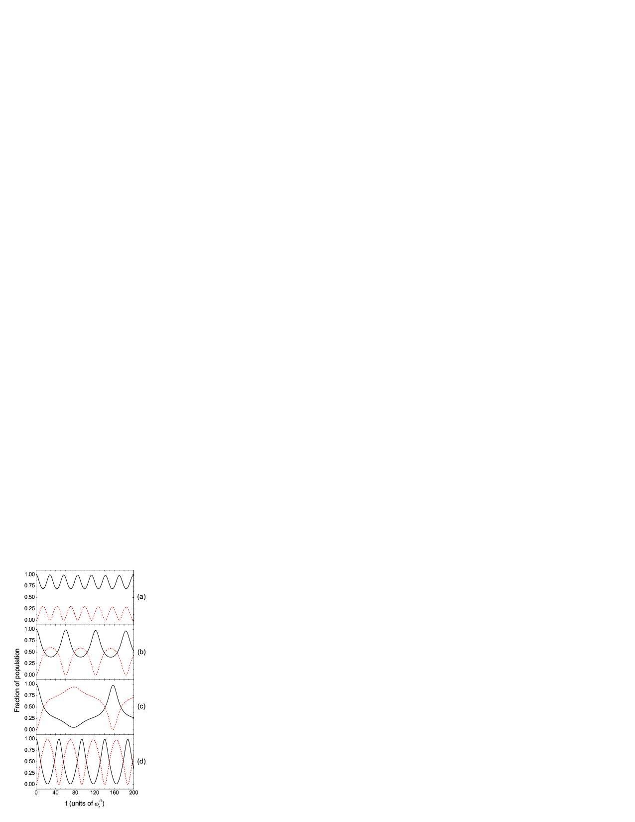
Figure 1: (Color online) Populations of the ground state $n_{0}$ (solid line) and excited state $\{100\}$ $n_{p}$ (dashed line) as a function of time for $\lambda=0.2$ and $g_{0}=70$ with (a) $a/a_{0}=0.7$ and $\delta=0$; (b) $a/a_{0}=0.7$ and $\delta=0.04$; (c) $a/a_{0}=0.72$ and $\delta=0.04$; (d) $a/a_{0}=1$ and $\delta=0.04$

The solutions demonstrate different behaviors of the state populations. For $a/a_{0}=0.7$ and $\delta=0$, Fig.1(a), the populations display small oscillation amplitudes, with a considerably larger population in the ground state. Increasing the detuning to $\delta=0.04$ results in the behavior shown in Fig.1(b). Although on average atoms stay longer in the ground state, for some intervals of time $n_{p}$ is larger than $n_{0}$. Changing the amplitude to $a/a_{0}=0.72$ and maintaining $\delta=0.04$, as in Fig.1(c), yields a very different temporal behavior. Atoms now stay longer in the excited state rather than in the ground state. The shape of the functions shows the inherent nonlinearity of the system. If the amplitude is increased further to $a/a_{0}=1$, with $\delta=0.04$, as in Fig. 1(d), the system shows a full population inversion. For certain times, when the mode population fully migrates from the ground $\{000\}$ to the excited $\{100\}$ state, it is possible to have a pure condensate in the coherent topological excited mode.

A convenient way to quantify the population behavior is through the introduction of an order parameter $\eta$, defined as the difference between the time-averaged populations for both states eta ; ramos ,

$$\eta=\bar{n}_{0}-\bar{n}_{p}.$$ (16)

Here, the average of each population is performed over the full cycle of an oscillation.

The above order parameter $\eta$ displays a nontrivial behavior when the ratio $a/a_{0}$ is modified. For different detunings, the variation of $\eta$ as a function of the ratio $a/a_{0}$ is presented in Fig.2.

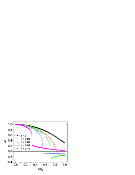
Figure 2: (Color online) Order parameter $\eta$ as a function of the ratio $a/a_{0}$, for different detunings showing a phase-transition like behavior.

The variation of $\eta$ vs. $a/a_{0}$ can be smooth, when $\delta\leq 0.03$, or can show sudden changes, when $\delta>0.03$. Smaller values of $a/a_{0}$ keep atoms preferably in the ground state. For some critical value of $a/a_{0}$, $\eta$ becomes negative, which means that BEC stays longer with a larger population in the excited state than in the ground state. This situation is ideal for detecting the formation of topological modes. Step like behavior observed on $\eta$ is not surprising for a nonlinear system. For example, the classical driven anharmonic oscillator landau exhibits a shift on its resonance curve, which we also observe in our system ramos pla . This shift for a large driven strength can result in a bistable behavior. In our system that appears as a step like response with $\eta$. This bistability appears only for positive detunings, as observed in our calculation. Negative detunings follows a smooth curve without step occurrence.

An important question is the feasibility of the experimental creation of such coherent modes. The main parameter here is $a/a_{0}$. It shows us that this value is strongly dependent on the Feshbach resonance width $\Delta$, characteristic of each type of atoms. For systems with small $\Delta$, the required value of $a/a_{0}$ for obtaining the transition in $\eta$ will occur only for $B_{0}\approx B_{res}$. In this case, the necessary condition $b\ll B_{res}-B_{0}$ can only be fulfilled for very small values of $b$, which creates an extra difficulty with the present techniques of magnetic field control strecker02 ; errico07 . As an experimentally realistic example, let us consider the case of $b=0.1(B_{res}-B_{0})$ and $a/a_{0}=0.8$, which corresponds to the atomic parameters listed in Table 1. Setting $g_{0}=70$, $\omega_{r}=2\pi\times 120\,$Hz, we obtain a value of $b$ of $0.9\,G$ for ⁸⁵Rb, and of $0.02\,G$ for ⁸⁷Rb, which would be difficult to control. On the other hand, $10\,G$, for ⁷Li, and $4.55\,G$, for ³⁹K, are values that can be realized with present technical capabilities strecker02 ; errico07 .

Let us consider now a condensate containing $10^{5}$ ⁷Li atoms in a trap with radial frequency $\omega_{r}=2\pi\times 120\,$Hz, $g_{0}=70$, and $\lambda=0.2$. With these conditions, the transition frequency is $\omega_{p0}=\omega_{100,0}=2\pi\times 209.6\,$Hz. Also, together with the information from Table 1, Eqs. (5) and (15), we obtain the bias magnetic field $B_{0}~{}=~{}632.5\,G$ and the amplitude $b=11.68\,a/a_{0}$. Then, we observe the critical values for $b$ ranging from $4\,G$ for a detuning $\omega-\omega_{p0}=2\pi\times 21\,$Hz to $10.5\,G$, for $\omega-\omega_{p0}=2\pi\times 6.3\,$Hz. Such oscillating amplitudes correspond to less than $1\%$ of the total bias field $B_{0}$.

Atom	$B_{res}(G)\;$	$\;\Delta(G)$	$\;a_{nr}\;$	$\;B_{0}(G)\;$	$\;b(G)\;$	$\;a_{0}$	$\;N(\times 10^{4})$
85Rb	155.0	10.7	-443	164.4	-0.9	63	0.2
87Rb	1007.34	0.17	100	1007.53	0.02	11	0.9
7Li	735	-113	-27.5	636	10	3.9	9.3
39K	403.4	-52	-23	357.9	4.55	3.3	4.7

Table 1: Amplitudes $B_{0}$ and $b$ of the magnetic field for four different species of atoms . We set $g_{0}=70$, $\lambda=0.2$, $a/a_{0}~{}=~{}0.8$ and $b=0.1(B_{res}-B_{0})$. Scattering length is expressed in units of the Bohr radius. Data for ⁸⁵Rb were obtained in Ref. claussen96 ; for ⁸⁷Rb, Ref. marte02 ; for ⁷Li, Ref. strecker02 ; for ³⁹K, Ref. errico07 .

A final point to be addressed concerns losses introduced by collisions, specially near a Feshbach resonance. With an off-resonant magnetic field, the dominant loss mechanism is a three body collision, whereas close to the resonance, the molecular formation dominates the atom loss mechanism stenger99 . Although the fields considered in Table 1 and in the ⁷Li example above are within the resonance linewidth, they are far enough to the resonance, then we consider three body collision as the main loss mechanism. In the case of ⁷Li, that the resonance linewidth is large, as we are in the border of this linewidth, the loss rate is very small, as shown in Ref. strecker02 . So, we can neglect the atom loss, specially because we apply the magnetic field in a short period of time.

IV Discussion

In conclusion, we have shown that using a magnetic modulation field, applied to a trapped Bose-condensed gas, it is possible to transfer the atomic population from the ground state to an excited state, producing a nonground-state condensate. The time averaged population imbalance between the ground and excited states represents an order parameter, which demonstrates an interesting behavior as a function of the modulation amplitude. Depending on the detuning, the behavior of $\eta$ can be either smooth or rather abrupt. This is the consequence of the strong nonlinearity of the interactions. For some range of detunings, $\eta$ becomes negative above a critical value of the modulation amplitude. This occurs because of the population inversion realized during the process of the mode excitation. Larger detunings and out-of-resonance modulations keep the population in the ground state and no population inversion is observed. Numerical calculations, accomplished for ⁷Li atoms, show that the values for the amplitude and modulation of the bias field are within realistic experimental conditions.

The justification of the approach for generating nonlinear coherent modes by the resonant modulation of an alternating field has been explained in detail in our previous publications nonground ; yyb ; eta ; yukalov03a ; yukalov03b . It would be unreasonable to repeat here all this justification in full. However, for the convenience of interested readers, we recall in brief some important points.

When a system is subject to the action of a time-dependent external field $V(t)$, alternating with a frequency $\omega$, then there exist two principally different situations, depending on the temporal alternation being either slow or fast zaslavsky . Respectively, there occur two different physical cases.

If the temporal variation is slow, such that the alternation frequency $\omega$ is much smaller than the characteristic system energy $E$, then one says that the perturbation is adiabatic zaslavsky . For a quantum-mechanical system, the energy $E$ is an eigenvalue of the system Hamiltonian $H$. When the latter varies slowly in time, so that the variation is adiabatic, then the adiabatic picture is in order, with the eigenvalues $E(t)$ and related eigenfunctions $\varphi(t)$ slowly varying in time. For such an adiabatic variation, the notion of nonlinear coherent modes is not of much use.

A principally different situation occurs, when the temporal variation is fast, so that $\omega$ is in resonance with one of the transition frequencies $\omega_{ij}\equiv(E_{i}-E_{j})/\hbar$. It is exactly this case that is considered in the present paper. Then the solutions of the stationary equation $H_{0}\varphi_{j}=E_{j}\varphi_{j}$ define the nonlinear coherent modes $\varphi_{j}$. Constructing a closed linear envelope, spanning the total set $\{\varphi_{j}\}$, one gets the Hilbert space ${\cal H}\equiv{\rm Span}\{\varphi_{j}\}$, with the typical property richtmyer that any function from ${\cal H}$ can be expanded over the set $\{\varphi_{j}\}$. The latter set forms a total basis yyb ; zhidkov , over which the solution of Eq. (6) can be expanded as in Eq. (9). Looking for the solution of Eq. (6) in the form of expansion (9), we employ the method of the parameter variation. Separating in expansion (9) the time-dependent coefficient function into two factors, the fastly oscillating exponential $\exp(-iE_{j}t/\hbar)$, and the slowly varying envelope $c_{j}(t)$, we can use the averaging techniques bogolubov and the scale separation approach yukalov96 ; yukalov00 . A similar technique in optics is called the slowly-varying amplitude approximation [32]. Substituting expansion (9) into Eq. (6) and involving the averaging techniques [29–31], we obtain Eqs. (11) for $c_{n}(t)$. This procedure is the same as has been done in Refs. [10,11].

In this way, one should not confuse the adiabatically slow variation of an external field, when the mode profiles and energies are certainly changing in time, and the fast resonant field oscillation, when the fractional mode populations vary between the stationary coherent modes. In the latter case, the solution to Eq. (6) can be represented in form (9) and the averaging techniques are applicable, yielding Eqs. (11) for the coefficient functions. The situation here is equivalent to the resonant excitation of an atom, as is discussed in Refs. [24,25]. In the same way as for an atom, the external resonant field should not be too strong in order not to disturb the energy-level classification. For this, it is sufficient to take the modulation amplitude $b$ in Eq. (3) appropriately small, which is always possible.

It is important to stress that the averaging technique, employed for deriving the equations for the fractional mode coefficients $c_{n}(t)$, is a well justified method based on rigorous mathematical theorems [29]. Therefore, this method does not require some other justifications.

Moreover, the results, obtained by means of the averaging techniques, when treating the generation of the nonlinear coherent modes by a resonant alternating field, have been thoroughly compared with the results of the direct numerical simulation of the Gross-Pitaevskii equation in Refs. [33,34]. Both ways of treating the problem have been found to be in a very good quantitative agreement.

In a real experiment, of course, a modulation, even being perfectly resonant, might, nevertheless, lead to heating, when the neighboring nonresonant levels become essentially involved in the process. This means that such a resonant mode generation can be effective only during a finite time. This problem has been analyzed in detail earlier [11,35], where it has been found that, taking the modulation amplitude sufficiently small, it is feasible to avoid heating during the lifetime of atoms inside a trap. For instance, the heating time was estimated [11,35] to be of order $10-100$ s.

The nonground-state nonlinear coherent modes are often termed topological, since the wavefunctions of different modes possess drastically different spatial shapes, with a different number and location of zeros. As an example, we can recall the wavefunctions of the first excited modes for atoms in a harmonic trap, found in Refs. [11,24]. These functions $\psi_{nmk}(x_{r},\varphi,x_{z})$, represented in dimensionless units of Eq. (14), are labelled by the quantum numbers $n$, $m$, and $k$ and are the functions of the dimensionless cylindrical variables $x_{r},\varphi$, and $x_{z}$. The ground-state wavefunction is

$$\psi_{000}=\left(\frac{u_{000}^{2}v_{000}}{\pi^{3}}\right)^{1/4}\;\mbox{e}^{-\left(u_{000}x_{r}^{2}+v_{000}x_{z}^{2}\right)/2}\;.$$

The radial dipole mode has the form

$$\psi_{100}=\left(\frac{u_{100}^{2}v_{100}}{\pi^{3}}\right)^{1/4}\left(u_{100}x_{r}^{2}-1\right)\;\mbox{e}^{-\left(u_{000}x_{r}^{2}+v_{000}x_{z}^{2}\right)/2}\;.$$

The vortex mode is also a possible stationary solution

$$\psi_{010}=u_{010}\left(\frac{v_{010}}{\pi^{3}}\right)^{1/4}x_{r}\;\mbox{e}^{i\varphi}\;\mbox{e}^{-\left(u_{000}x_{r}^{2}+v_{000}x_{z}^{2}\right)/2}\;.$$

And the axial dipole mode is

$$\psi_{001}=\left(\frac{4u_{001}^{2}v_{001}^{3}}{\pi^{3}}\right)^{1/4}x_{z}\;\mbox{e}^{-\left(u_{000}x_{r}^{2}+v_{000}x_{z}^{2}\right)/2}\;.$$

The quantities $u_{nmk}$ and $v_{nmk}$ here are defined by the optimization conditions and depend on all system parameters (see calculational details in Refs. [11,24]). As is evident, the spatial shapes of atomic clouds, described by $|\psi_{nmk}|^{2}$, are principally different for different quantum numbers.

If the scattering length is modulated according to Eq. (4), then the resulting Eq. (6) acquires the additional term (8) playing the role of a modulating field. Therefore the mechanism of generating nonground-state modes is the same for both the cases, whether the additional term is caused by the trap modulation or by the scattering-length modulation. In any case, the general structure of Eqs. (6) to (8) is similar for both these setups.

The main difference between the methods of generating nonlinear coherent modes by the trap modulation or by the scattering-length modulation is as follows. In the method of the trap modulation, by choosing the appropriate spatial dependence of the modulating field $V({\bf r},t)$, it is possible to generate any type of modes. While, in the method of the scattering-length modulation, only those modes can be excited, for which the integrals in Eq. (12) are nonzero. For example, in the case of cylindrically symmetric harmonic trap with potential (13), the integrals $I_{0,p,p}$, $I_{0,0,p}$, $I_{p,0,0}$, and $I_{p,p,0}$, in which $p$ implies a set $\{n,m,k\}$, vanish for the vortex mode $\psi_{p}=\psi_{010}$ and for the axial dipole mode $\psi_{p}=\psi_{001}$. Hence, in these cases, the vortex and the axial dipole modes cannot be excited by modulating the scattering length. However, the radial dipole mode $\psi_{100}$ can be generated by this method, since the related integrals (12) are nonzero. This is why, we have considered here exactly this case. A way out of the problem, which would allow for the generation of other modes, including the vortex mode, could be by employing a nonsymmetric trapping potential.

- (1) L. Pitaevskii and S. Stringari, Bose-Einstein Condensation (Clarendon, Oxford, 2003).
- (2) P. W. Courteille, V.S. Bagnato, and V.I. Yukalov, Laser Phys. 11, 659 (2001).
- (3) J.O. Andersen, Rev. Mod. Phys. 76, 599 (2004).
- (4) V.I. Yukalov and M.D. Girardeau, Laser Phys. Lett. 2, 375 (2005).
- (5) H. Saito, R. G. Hulet, and, M. Ueda, Phys. Rev. A 76, 053619 (2007);
- (6) T. Koch et. al, Nature Phys. 4, 218 (2008).
- (7) M. Greiner et. al, Nature 426, 537 (2003).
- (8) E. A. Donley et. al, Nature 412, 295 (2001).
- (9) S. K. Adhikari, Phys. Rev. A 71, 053603 (2005).
- (10) V.I. Yukalov, E.P. Yukalova, and V.S. Bagnato, Phys. Rev. A 56, 4845 (1997);
- (11) V.I. Yukalov, E.P. Yukalova, and V.S. Bagnato, Phys. Rev. A 66, 043602 (2002).
- (12) J. R. Abo-Shaeeret. al, Science 292, 476 (2001);
- (13) P. Rosenbusch, V. Bretin, and J. Dalibard, Phys. Rev. Lett. 89, 200403 (2002);
- (14) V.I. Yukalov, E.P. Yukalova, and V.S. Bagnato, Laser Phys. 12, 231 (2002);
- (15) E. Kreyszig, Maple Computer Guide: a Self-Contained Introduction (Wiley, New York, 2001).
- (16) E. R. F. Ramos, L. Sanz, V. I. Yukalov, and, V. S. Bagnato, Phys. Rev. A 76, 033608 (2007).
- (17) L. D. Landau and E. M. Lifshitz, Mechanics (Pergamon Press, Oxford, 1960).
- (18) E. R. F. Ramos, L. Sanz, V. I. Yukalov, and, V. S. Bagnato, Phys. Lett. A 365, 126 (2007).
- (19) K. E. Strecker et. al, Nature 417, 150 (2002).
- (20) C. D’Errico et. al, New J. Phys. 9, 223 (2007).
- (21) N.R. Claussen, Ph.D. Thesis (University of Colorado, Boulder, 1996).
- (22) A. Marte et.al, Phys. Rev. Lett. 89, 283202 (2002).
- (23) J. Stenger et.al, Phys. Rev. Lett. 82, 2422 (1999).
- (24) V.I. Yukalov, E.P. Yukalova, and V.S. Bagnato, Laser Phys. 13, 551 (2003).
- (25) V.I. Yukalov, E.P. Yukalova, and V.S. Bagnato, Laser Phys. 13, 861 (2003).
- (26) G.M. Zaslavsky and R.G. Sagdeev, Introduction to Nonlinear Physics (Nauka, Moscow, 1988).
- (27) R.D. Richtmyer, Principles of Advanced Mathematical Physics (Springer, New York, 1981).
- (28) P.E. Zhidkov, Nonlin. Anal. 52, 737 (2003).
- (29) N.N. Bogolubov and Y.A. Mitropolsky, Asymptotic Methods in the Theory of Nonlinear Oscillations (Gordon and Breach, New York, 1961).
- (30) V.I. Yukalov, Phys. Rev. B 53, 9232 (1996).
- (31) V.I. Yukalov and E.P. Yukalova, Phys. Part. Nucl. 31, 561 (2000).
- (32) B.W. Shore, Theory of Coherent Atomic Excitation (Wiley, New York, 1990).
- (33) V.I. Yukalov, K.P. Marzlin, and E.P. Yukalova, Phys. Rev. A 69, 023620 (2004).
- (34) V.I. Yukalov, K.P. Marzlin, and E.P. Yukalova, Laser Phys. 14, 565 (2004).
- (35) V.I. Yukalov, Laser Phys. Lett. 3, 406 (2006).