A Lagrangean formalism for
Hermitean matrix models

R. Flume¹, J. Grossehelweg², A. Klitz¹

¹ Physikalisches Institut, Universität Bonn,

Nußallee 12, 53115 Bonn, Germany

² DESY Theory Group, DESY Hamburg,

Notkestr. 85, 22603 Hamburg, Germany

Eynard’s formulation of Hermitean 1-matrix models in terms of intrinsic quantities of an associated hyperelliptic Riemann surface is rephrased as a Lagrangean field theory of a scalar particle propagating on the hyperelliptic surface with multiple self-interactions and particle-source-interactions. Both types of interaction take place at the branch points of the hyperelliptic surface.

1 Introduction

The conceptual and practical understanding of some random matrix models has been advanced significantly by the seminal work of Eynard [4]. This author introduced an elegant new approach to the topological expansion of Hermitean 1-matrix models based on the intrinsic notions of a hyperelliptic Riemann surface which is—as spectral surface—attached to the matrix model. The new approach has been further elucidated in [5] and applied to 2-matrix models in [6] and [7]. It has moreover been shown in [8] that one may abstract from the framework of matrix models to the construction of new invariants attached to more general Riemann surfaces (mimicking the topological expansion of matrix models). This brings into focus [8] new subjects as Kontsevich’s matrix model for intersection numbers [9], topological string theory [10], [11], [12] and [13], as well as further applications to mathematical subjects, as the recursive determination of Weil-Petersson volumes [14], [15] and a conjectural matrix model representation of Hurwitz numbers [16].

The purpose of this note is to show that Eynard’s elegant construction can be deciphered into a non-elegant effective Lagrangean formalism. We will concentrate here on Hermitean 1-matrix models—but we hope that our methods will also apply in some of the instances mentioned above. The Lagrange to be constructed will be that of a scalar field propagating on a hyperelliptic Riemann surface (i.e. the Riemann surface given as the spectral curve associated with the matrix model). The corresponding ’vacuum graphs’ of the Gell-Mann-Low expansion and the graphs for the Green’s functions will be shown to represent the free energy and the correlations of resolvent operators resp. of the matrix model. The self-interaction of the scalar field and its interaction with background sources will be given as formal infinite power series, which receive ’short distance’ (see below) corrections throughout the loop expansion of the effective theory. This latter expansion will be identified with the topological expansion of the matrix model.
The unpublished work [19] has been fused into the present article.

The plan of the paper is as follows: In section 2 we collect some technical material concerning Hermitean 1-matrix models taken from the literature [1] - [4], [17]. (Experts may skip this section.) Section 3 is devoted to the construction of the effective Lagrange in tree graph approximation which is identified with the leading large N order for the matrix model. In section 4 we discuss the non-leading terms of the matrix model topological expansion, i.e. the loop corrections in Lagrangean parlance. We end in section 5 with some conclusions.

2 Hermitean 1-matrix models

The partition function of Hermitean 1-matrix models ([1], [2]) is given by a (potentially formal) integral over Hermitean matrices

$$Z_{N}(t)=\int e^{-N\;{\rm tr}\;V(M)}\;dM\;,$$ (1)

$$dM=\underset{i}{\prod}\;dM_{ii}\;\;\underset{i<j}{\prod}\;Re\ dM_{ij}\;\;\underset{i<j}{\prod}\;Im\ dM_{ij}\;;$$

$M_{ii}$ are real variables; the potential $V(M)$ is given by $V(M)=\sum_{n\geq 1}t_{n}M^{n}$, with $t_{n}$ denoting some coupling constants. Ensuing averages are introduced as usual:

$$\langle f(M)\rangle=\frac{1}{Z}\int f(M)\;e^{-N\;{\rm tr}\;V(M)}\;dM.$$ (2)

The free energy $\mathcal{F}$ related to the partition function by $Z_{N}(t)=e^{\mathcal{F}}$ can formally be expanded in powers of $\frac{1}{N}$ (the so-called topological expansion)

$$\mathcal{F}=\sum_{h=0}^{\infty}N^{2-2h}\;\mathcal{F}^{(h)}.$$ (3)

Following well established paths [3] we introduce a derivative called the ’loop operator’

$$\frac{\partial}{\partial V(z)}=-\sum_{j=1}^{\infty}\frac{1}{z^{j+1}}\frac{\partial}{\partial t_{j}},$$ (4)

z denoting here a complex number. Connected correlators of the resolvent

$$W(z)=\frac{1}{N}tr\frac{1}{z-M}$$

are obtained by multiple application of the loop operator to the free energy

$$W_{n}(z_{1},\ldots,z_{n})=N^{2n-2}\langle W(z_{1})\ldots W(z_{n})\rangle_{\rm conn}=\frac{1}{N^{2}}\frac{\partial}{\partial V(z_{1})}\cdots\frac{\partial}{\partial V(z_{n})}\mathcal{F}.$$ (5)

The subscript ’conn’ refers to the connectedness of the correlator.
The correlation function $W_{n}$ inherits from the free energy a topological expansion

$$W_{n}(z_{1},\ldots,z_{n})=\sum_{h=0}^{\infty}N^{-2h}W_{n}^{(h)}(z_{1},\ldots,z_{n}).$$ (6)

It turned out that the most efficient tool for the determination of the partition function (the free energy resp.) and of the correlators of resolvents are the so-called loop identities, that is, Ward identities for invariance of the defining integrals under reparametrisations of the matrix model integration variables of the type

$$\delta M=\varepsilon\frac{1}{z-M}$$

with $\varepsilon$ denoting an infinitesimal real parameter and $z$ an arbitrary complex number. The invariance of the partition function under this variation leads to the identity

$$(W_{1}(z))^{2}+\frac{1}{N^{2}}W_{2}(z,z)=\frac{1}{N}\langle{\rm tr}\frac{V^{\prime}(M)}{z-M}\rangle.$$ (7)

The l.h.s. of the latter equation derives from the variation of the measure in eq. (1) under the variation (6) whereas the r.h.s. derives from the variation of the integrand $\exp(-N\;{\rm tr}\,V(M))$. Applying to eq. (7) the loop operator—or equivalently, starting from a more involved variation substituting instead of eq. (6)

$$\delta M=\varepsilon\frac{1}{z_{1}-M}\prod_{j>1}{\rm tr}\frac{1}{z_{j}-M}$$

one can deduce further identities for multipoint functions. Eynard [4] uses those identities to establish for the correlation functions and finally also for the higher order corrections to the free energy a recursive procedure giving rise to a trivalent graphical representation (cf. [5] in the latter context).
Invariance under the unitary group $U(N)$ may be exploited to reduce all $N^{2}$-dimensional integrals above to $N$-dimensional integrals over eigenvalues of the Hermitean matrices. The partition function, eq. (1), in particular becomes then [1]

$$Z_{N}(t)=\int\prod_{i=1}^{N}d\lambda_{i}\prod_{i<j}(\lambda_{i}-\lambda_{j})^{2}\prod_{i}e^{-NV(\lambda_{i})},$$ (8)

where we have skipped—for convenience—on the r.h.s. of (8) the volume factor of the unitary group. We assume (as [1]-[4]) that the eigenvalues are, for large values of $N$, concentrated on a finite number of compact intervals on the real axis, say

$$\bigcup_{l=1}^{s}\;A_{l}\mbox{ with }A_{l}=[a_{2l-1},a_{2l}],\ \ \ a_{1}<a_{2}<\ldots<a_{2s}$$

where the separate intervals $[a_{2l-1},a_{2l}]$ are supposed to be spread in the neighbourhood of diverse minima of the potential $V(\lambda)$. The spectral density $\rho_{N}(\lambda)$, concentrated on the above intervals, becomes a continuous function $\rho(\lambda)$ in the large $N$ limit. The expectation value of the resolvent reads in terms of this distribution as

$$W_{1}(p)=\int d\lambda\frac{\rho(\lambda)}{p-\lambda}$$ (9)

and the loop equation (7) becomes

$$\oint\limits_{\mathcal{C}}\frac{d\omega}{2\pi i}\frac{V^{\prime}(\omega)}{p-\omega}W_{1}(\omega)=(W_{1}(p))^{2}+\frac{1}{N^{2}}W_{2}(p,p).$$ (10)

The contour $\mathcal{C}$ of the integral on the l.h.s. is supposed to encircle in the complex plane the support of the spectral measure, but not the point $p$. The second term on the r.h.s. of (10) drops out in leading order of the large $N$ expansion and one is left with the quadratic equation for the leading part $W_{1}^{(0)}$,

$$(W_{1}^{(0)}(p))^{2}=\oint\limits_{\mathcal{C}}\frac{d\omega}{2\pi i}\frac{V^{\prime}(\omega)}{p-\omega}W_{1}^{(0)}(\omega)=\int d\omega\frac{V^{\prime}(\omega)-V^{\prime}(p)+V^{\prime}(p)}{p-\omega}\rho(\omega)$$

$$=V^{\prime}(p)\;W_{1}^{(0)}(p)-\int d\omega\frac{V^{\prime}(p)-V^{\prime}(\omega)}{p-\omega}\rho(\omega)=V^{\prime}(p)\;W_{1}^{(0)}(p)+f(p),$$ (11)

where $f(p)$ denotes a polynomial of a degree one less than the degree of $V^{\prime}(\omega)$. $W_{1}^{(0)}(p)$ is given as solution of the preceding quadratic equation,

$$W_{1}^{(0)}(p)=\frac{1}{2}V^{\prime}(p)-\frac{1}{2}\sqrt{(V^{\prime}(p))^{2}+4f(p)},$$ (12)

the sign of the square root term being dictated by the stipulated asymptotic behaviour $W_{1}^{(0)}(p)\sim\frac{1}{p}$, $p\rightarrow\infty$. The expectation value of the resolvent is in this way related to a hyperelliptic Riemann surface given by the equation

$$y^{2}=(V^{\prime}(\lambda))^{2}+4f(\lambda).$$ (13)

One is free to choose $f$ s.t. the polynomial on the r.h.s. has a finite even number, say $2s$, of simple zeros in accordance with the above assumption on the support of the spectral density—besides an appropriate number of double zeros, s.t. $y$ reads as

$$y=M(\lambda)\tilde{y},$$ (14)

$$\tilde{y}^{2}=\prod_{i=1}^{2s}(\lambda-a_{i}),$$ (15)

where $\tilde{y}$ now represents a reduced hyperelliptic surface [5] of the same genus $g=s-1$ as $y$. The polynomial $M(\lambda)$ can be seen by inspection of the loop equation (11) to be given by a Cauchy contour integral (cf. [3])

$$M(\lambda)=\oint\limits_{\mathcal{C_{\infty}}}\frac{d\omega}{2\pi i}\frac{1}{\omega-\lambda}\frac{V^{\prime}(\omega)}{\sqrt{\prod_{i=1}^{2s}(\omega-a_{i})}}$$ (16)

where $\mathcal{C_{\infty}}$ denotes a contour encircling all branch points $a_{i}\ ,i=1,\ldots,2s$ and $\lambda$. $W_{1}^{(0)}(\lambda)$ is found similarly

$$W_{1}^{(0)}(\lambda)=\frac{1}{2}\oint\limits_{\mathcal{C}}\frac{d\omega}{2\pi i}\frac{V^{\prime}(\omega)}{\lambda-\omega}\sqrt{\frac{\prod_{i=1}^{2s}(\lambda-a_{i})}{\prod_{j=1}^{2s}(\omega-a_{j})}}$$

where $\mathcal{C}$ now encircles the branch points but not $\lambda$.
To fix the positions of the branch points one has to impose particular boundary conditions. Following [4], [17] we choose those to be given by ’filling fractions’

$$\varepsilon_{l}=\frac{1}{2}\oint\limits_{A_{l}}\frac{d\lambda}{2\pi i}y(\lambda)$$

which are the relative weights of the various spectral intervals. The insertion of the topological expansion (6) into the loop equation (10) gives rise to

$$(\hat{\mathcal{K}}-2W_{1}^{(0)}(p))W_{1}^{(h)}(p)=\sum_{h^{\prime}=1}^{h-1}W_{1}^{(h^{\prime})}(p)W_{1}^{(h-h^{\prime})}(p)+W_{2}^{(h-1)}(p,p),$$ (17)

$$\hat{\mathcal{K}}f(p)=\oint\limits_{\mathcal{C}}\frac{d\lambda}{2\pi i}\frac{V^{\prime}(\lambda)}{p-\lambda}f(\lambda).$$

The solution of (17) under the condition

$$\oint\limits_{A_{j}}dx_{1}W_{2}(x_{1},x_{2})=0\ \ \ \ \ \ \ \forall j$$

(stipulating that the filling fractions are to be chosen independently of the form of the interaction potential $V(t)$) is found, [4], to be

$$W_{1}^{(h)}(p)=\sum_{i=1}^{2s}\underset{x\rightarrow a_{i}}{\rm Res}\frac{dS(p,x)}{dp}\frac{1}{y(x)}\left(\sum_{m=1}^{h-1}W_{1}^{(h-m)}(x)W_{1}^{(m)}(x)+W_{2}^{(h-1)}(x,x)\right)$$ (18)

with $dS(p,x)$ denoting a meromorphic one form with respect to the variable $p$ and a multivalued meromorphic function in $x$ on the reduced Riemann surface (15). $dS$ is characterized uniquely by the following properties:

$$dS(x,x^{\prime}) \underset{x\rightarrow x^{\prime}}{=} \frac{dx}{x-x^{\prime}}+\mbox{ finite},$$

$$dS(x,x^{\prime}) \underset{x\rightarrow\overline{x^{\prime}}}{=} -\frac{dx}{x-x^{\prime}}+\mbox{ finite},$$

($\overline{x}$ denoting the hyperelliptic involution of $x$) where the quoted singularities are the only ones on the reduced surface, and

$$\oint\limits_{A_{j}}dS(x,x^{\prime})=0\ \ \ \ \forall\;j=1,\ldots,s-1.$$

The explicit expression for $dS(x,x^{\prime})$ is

$$dS(x,x^{\prime})=\frac{\sqrt{\sigma(x^{\prime})}}{\sqrt{\sigma(x)}}\left(\frac{1}{x-x^{\prime}}-\sum_{j=1}^{s-1}C_{j}(x^{\prime})L_{j}(x)\right)dx$$ (19)

$$\mbox{with\ \ }C_{j}(x^{\prime})=\frac{1}{2\pi i}\oint\limits_{A_{j}}\frac{dx}{\sqrt{\sigma(x)}}\frac{1}{x-x^{\prime}}\mbox{ and }\sigma(x)=\prod_{i=1}^{2s}(x-a_{i}).$$

$L_{j}(x)$ denote polynomials which are constitutive parts of the normalized holomorphic 1-forms of the reduced surface,

$$\omega_{j}(x)=\frac{L_{j}(x)}{\sqrt{\sigma(x)}}dx$$

$$\oint\limits_{A_{l}}\omega_{j}(x)=2\pi i\delta_{jl}\mbox{\ for \ }l,j\in{1,\ldots,s-1}.$$

One needs for the resolution of the recursion, eq. (18), in explicit form the two-point function $W_{2}^{(0)}(p,q)$. This is found as solution of the loop equation for the two-point function—which emerges from another application of the loop operator to both sides of eq. (11)—in terms of the ’Bergmann kernel’ $B(p,q)$ (cf. [4]):

$$W_{2}^{(0)}(p,q)=\frac{B(p,q)}{dq\ dp}-\frac{1}{(p-q)^{2}}.$$ (20)

$B$ is a symmmetric bidifferential on the reduced surface with a unique second order pole at the coincidence point $p=q$, $B(p,q)=(\frac{dp\;dq}{(p-q)^{2}}+{\rm finite})$ for $p\rightarrow q$ and satisfying the normalization conditions

$$\oint\limits_{q\in A_{j}}B(p,q)=0,\ j=1,\ldots,s-1.$$

The Bergmann kernel is related to the above introduced differential $dS$ as follows:

$$B(p,q)=\frac{1}{2}\frac{\partial}{\partial q}\left(\frac{dp}{p-q}+dS(p,q)\right)dq.$$ (21)

The solution of the recursion relation (18) and its generalization for multipoint correlation functions in terms of $dS(p,q)$, $B(p,q)$, $y(q)$, i.e. in terms of intrinsic quantities of the hyperelliptic surfaces (14) and (15) is due to Eynard. For details of this formalism we refer to the original work [4] and [5], [8].

3 The planar approximation in terms of tree graphs of an effective Lagrange

The determination of the multipoint correlators of resolvents in leading order of $\frac{1}{N}$ may either proceed by inspection of the multipoint generalisation of the loop equation (11)—this approach has been followed by Eynard [4]—or may be achieved by repeated application of the loop operator to the above noted result, eq. (20), for the resolvent two-point correlation function. That is, one applies the loop operator either to the loop equation or to its solution. We will follow here the second route.
The variation of the Bergmann kernel, eq. (21), due to an infinitesimal change of the branch points of the underlying hyperelliptic surface is given by one of Rauch’s variational formulas [18]:

$$\delta B(p,q)=\frac{1}{2}\sum_{j}B(p,[a_{j}])B(q,[a_{j}])\delta a_{j}.$$ (22)

$B(p,[a_{j}])$ governs the asymptotic behaviour of $B(p,q)$ in $q$ near $a_{j}$:

$$B(p,[a_{j}])=\left.2\frac{\sqrt{q-a_{j}}B(p,q)}{dq}\right|_{q\rightarrow a_{j}}.$$

In the following we will use

$$\widetilde{B}(p,q)=\frac{B(p,q)}{dp\;dq}-\frac{1}{2}\frac{1}{(p-q)^{2}}$$

and

$$\widetilde{B}(p,[a_{j}])=2\oint\limits_{a_{j}}\frac{dz}{2\pi i}\frac{\widetilde{B}(p,z)}{(z-a_{j})^{1/2}}.$$

Rauch’s formula is to be combined with an expression for $\frac{\delta a_{j}}{\delta V(p)}$. The latter is found by first noting the relation, [5],

$$\frac{\delta y(q)}{\delta V(p)}=-2\widetilde{B}(p,q)$$ (23)

and to match this with the asymptotic behaviour $y(q)=y([a_{i}])\sqrt{q-a_{i}}+\mathcal{O}((q-a_{i})^{3/2})$, which implies

$$\left.\frac{\delta y(q)}{\delta V(p)}\right|_{q\rightarrow a_{i}}=-\frac{1}{2}y([a_{i}])\frac{1}{\sqrt{q-a_{i}}}\frac{\delta a_{i}}{\delta V(p)}+\mathcal{O}(\sqrt{q-a_{i}}).$$ (24)

Eqs. (23) and (24) lead us to

$$\frac{\delta a_{i}}{\delta V(p)}=\frac{2\widetilde{B}(p,[a_{i}])}{y([a_{i}])}$$ (25)

which with eq. (22) gives rise to

$$W_{3}^{(0)}(p_{1},p_{2},p_{3})=\frac{\delta}{\delta V(p_{3})}W_{2}^{(0)}(p_{1},p_{2})=\sum_{i=1}^{2s}\frac{\widetilde{B}(p_{1},[a_{i}])\widetilde{B}(p_{2},[a_{i}])\widetilde{B}(p_{3},[a_{i}])}{y([a_{i}])}.$$ (26)

Figure 1: Three point function $W_{3}^{(0)}$. The vertex factor is $1/y_{1,i}$.

We will use the notations

$$\ \ \ \ \ \ \ \ \ \ B_{i}^{f}(p) = 2\oint\limits_{a_{i}}\frac{dz}{2\pi i}\frac{\widetilde{B}(p,z)}{(z-a_{i})^{f+1/2}}\ \ \ \ \ \ \ \ \ \ \ \ \ \ \ \ \ \ \ \ \ \ \ \ \ \ \ \ \ \ \ \ \ \ \ \ \ \ \ \ \ {\rm(27a)}$$

$$B_{i,j}^{f,g} = 4\oint\limits_{a_{i}}\frac{dz}{2\pi i}\oint\limits_{a_{j}}\frac{dz^{\prime}}{2\pi i}\frac{\widetilde{B}(z,z^{\prime})}{(z-a_{i})^{f+1/2}(z-a_{j})^{g+1/2}}\ \ \ \ \ \ \ \ \ \ \ \ \ \ \ \,{\rm(27b)}$$

$$y_{f,i} = \oint\limits_{a_{i}}\frac{dz}{2\pi i}\frac{y(z)}{(z-a_{i})^{f+1/2}}.\ \ \ \ \ \ \ \ \ \ \ \ \ \ \ \ \ \ \ \ \ \ \ \ \ \ \ \ \ \ \ \ \ \ \ \ \ \ \ \ \ \ \!\>{\rm(27c)}$$

It will turn out that the collection of quantities (27a)-(27c) is complete in the sense that the resolvent correlators and the free energy can be expressed—as will be shown—to all orders in the topological expansion by those terms. One should note that (27b) is well defined also for $i=j$, since the order of the contours does not matter due to the fact that $B(p,q)$ has as single singularity a second order pole with residuum one. Straightforward calculations using eqs. (25) and (26) lead to the relations

$$\frac{\delta y_{f,i}}{\delta V(q)} = \big{(}\Delta_{1}(q)+\Delta_{2}(q)\big{)}(y_{f,i})$$

$$\big{(}\Delta_{1}(q)\big{)}(y_{f,i})=(2f+1)\frac{y_{f+1,i}}{y_{1,i}}B_{i}^{0}(q)\ \ \ \ \ \ \ \ \ \ \ \ \ \ \ \ \ {\rm(\ref{eq: y_fi variation}a)}$$

$$\big{(}\Delta_{2}(q)\big{)}(y_{f,i})=-B_{i}^{f}(q)\ \ \ \ \ \ \ \ \ \ \ \ \ \ \ \ \ \ \ \ \ \ \ \ \ \ \ \ \ \ \ \ \ {\rm(\ref{eq: y_fi variation}b)}$$

$$\frac{\delta B_{i}^{f}(p)}{\delta V(q)} = \big{(}\Delta_{3}(q)+\Delta_{4}(q)\big{)}(B_{i}^{f}(p))$$

$$\big{(}\Delta_{3}(q)\big{)}(B_{i}^{f}(p))=(2f+1)\frac{B_{i}^{f+1}(p)B_{i}^{0}(q)}{y_{1,i}}\ \ \ \ \ \ \ \ \ \ {\rm(\ref{eq: B_i^f variation}a)}$$

$$\big{(}\Delta_{4}(q)\big{(}B_{i}^{f}(p))=\sum_{j=1}^{2s}\frac{B_{i,j}^{f,0}B_{j}^{0}(p)B_{j}^{0}(q)}{y_{1,j}}\ \ \ \ \ \ \ \ \ \ \ \ \ \ \>{\rm(\ref{eq: B_i^f variation}b)}$$

$$\frac{\delta B_{i,j}^{f,g}}{\delta V(q)} = \big{(}\Delta_{5}(q)+\Delta_{6}(q)+\Delta_{7}(q)\big{)}(B_{i,j}^{f,g})$$

$$\big{(}\Delta_{5}(q)\big{)}(B_{i,j}^{f,g})=(2f+1)\frac{B_{i,j}^{f+1,g}B_{i}^{0}(q)}{y_{1,i}}\ \ \ \ \ \ \ \ \ \ \ \ \ \ \,{\rm(\ref{eq: B_ij^fg variation}a)}$$

$$\big{(}\Delta_{6}(q)\big{)}(B_{i,j}^{f,g})=(2g+1)\frac{B_{i,j}^{f,g+1}B_{j}^{0}(q)}{y_{1,j}}\ \ \ \ \ \ \ \ \ \ \ \ \ \ \ \!\!\;{\rm(\ref{eq: B_ij^fg variation}b)}$$

$$\big{(}\Delta_{7}(q)\big{)}(B_{i,j}^{f,g})=\sum_{k=1}^{2s}\frac{B_{i,k}^{f,0}B_{j,k}^{g,0}B_{k}^{0}(q)}{y_{1,k}}.\ \ \ \ \ \ \ \ \ \ \ \ \ \ \ \ \ \!\>{\rm(\ref{eq: B_ij^fg variation}c)}$$

The application of an operator $\Delta_{j}(q)$, $j=1,\ldots,7$ to expressions not noted above gives zero. It can also easily be verified that $\frac{\delta}{\delta V(q)}$ and $\frac{\delta}{\delta V(p)}$ are for arbitrary arguments $p$ and $q$ commuting operators acting on the basis (27a-c) (as it should be indeed). The 4-point function is found by application of $\frac{\partial}{\partial V(p)}$ (cf. eqs. (3) and (3)) to $W_{3}^{(0)}$. One finds:

$$\!\!\!\!\!\!\!\!\!\!\!\!\!\!W_{4}^{(0)}(p_{1},\ldots,p_{4})=\frac{\delta}{\delta V(p_{4})}W_{3}^{(0)}(p_{1},p_{2},p_{3})\hskip 85.35826pt$$ (31)

$$= \sum_{i,j=1}^{2s}\left(B_{i}^{0}(p_{1})B_{i}^{0}(p_{2})\left(\frac{1}{y_{1,i}}\right)B_{i,j}^{0,0}\left(\frac{1}{y_{1,j}}\right)B_{j}^{0}(p_{3})B_{j}^{0}(p_{4})\right.$$

$$+ B_{i}^{0}(p_{1})B_{i}^{0}(p_{3})\left(\frac{1}{y_{1,i}}\right)B_{i,j}^{0,0}\left(\frac{1}{y_{1,j}}\right)B_{j}^{0}(p_{2})B_{j}^{0}(p_{4})\left.\right.$$

$$+ \left.B_{i}^{0}(p_{1})B_{i}^{0}(p_{4})\left(\frac{1}{y_{1,i}}\right)B_{i,j}^{0,0}\left(\frac{1}{y_{1,j}}\right)B_{j}^{0}(p_{3})B_{j}^{0}(p_{2})\right)$$

$$+ \sum_{i=1}^{2s}\left(-3\frac{y_{2,i}}{y_{1,i}^{3}}\right)\prod_{r=1}^{4}B_{i}^{0}(p_{r})+\sum_{r=1}^{4}\sum_{i=1}^{2s}\left(\frac{1}{y_{1,i}^{2}}\right)B_{i}^{1}(p_{r})\prod_{\scriptstyle t=1\atop\scriptstyle t\neq r}^{4}B_{i}^{0}(p_{t}).$$

Eq. (26) and (31) designate the starting for an effective Lagrangean description of the resolvent operator correlation functions.

Figure 2: Various contributions to the 4-point function. (a) Second order contributions of the cubic interaction. (b)+(c) Genuine quartic interactions without and with a derivative field, the latter being indicated by a bar. The various vertex factors are not accounted for.

The most obvious hint from both equations is that the interactions are concentrated at the branch points $a_{i}$ , $i=1,\ldots,2s$ and that an interaction point is connected to the external resolvent operator by a ’propagator’ $B_{i}^{0}(p)$. The 3-point correlator can obviously be related to a cubic interaction:

$$S_{3}^{(0)}=\int\mathcal{L}_{3}^{(0)}(x)\;dx\ \ \mbox{ with }\ \ \mathcal{L}_{3}^{(0)}(x)=\frac{1}{y_{1}(x)}\frac{\varphi^{3}(x)}{3!}=\frac{1}{y_{1}}\frac{\varphi^{3}}{3!}$$ (32)

with the correspondences

$$\int dx=\sum_{i=1}^{2s}\Big{|}_{x=a_{i}},\ \ \ \ \ \ \ \ \ \ \ \ \ \ \ \ \ \ \ \ \ \begin{picture}(7.2,2.0)\put(0.6,2.2){\line(1,0){4.2}} \put(0.6,2.2){\line(0,-1){1.0}} \put(4.8,2.2){\line(0,-1){1.0}} \put(0.0,0.0){$\varphi(a_{i})\;\varphi(p)$} \end{picture}=B_{i}^{0}(p).$$

The first bracket on the r.h.s. of (31) represents then the second order contribution of the cubic interaction to the 4-point correlator where one propagator is exchanged between the interaction vertices at places $a_{i}$ and $a_{j}$. The second and third term on the r.h.s. of (31) are generated by quartic interactions as

$$S_{4}^{(0)(a)}=\int dx\left(-\frac{3y_{2}}{y_{1}^{3}}\right)\frac{\varphi^{4}}{4!}\equiv\sum_{i=1}^{2s}\left(-\frac{3y_{2,i}}{y_{1,i}^{3}}\right)\frac{\varphi^{4}(a_{i})}{4!}$$ (33)

and

$$S_{4}^{(0)(b)}=\int dx\frac{1}{y_{1}^{2}(x)}\frac{\varphi^{3}}{3!}\frac{\partial\varphi}{1!}\equiv\sum_{i=1}^{2s}\frac{1}{y_{1,i}^{2}}\frac{\varphi^{3}(a_{i})}{3!}\frac{\partial\varphi(a_{i})}{1!}$$ (34)

where the derivative $(\partial\varphi)_{i}=(\partial\varphi)(a_{i})$ gives rise to the factor $B_{i}^{1}(p_{0})$. The Lagrange resulting from these quartic interactions is

$$\mathcal{L}_{4}^{(0)}=\left(-3\frac{y_{2}}{y_{1}^{3}}\right)\frac{\varphi^{4}}{4!}+\left(\frac{1}{y_{1}^{2}}\right)\frac{\varphi^{3}\;\partial\varphi}{3!1!}.$$

We will have to make use of couplings with derivatives of arbitrary order: $B_{i}^{f}(p)$ will point to an $f$-th order derivative field at place $a_{i}$,

$$\begin{picture}(9.0,2.0)\put(2.6,2.5){\line(1,0){3.2}} \put(2.6,2.5){\line(0,-1){1.0}} \put(5.8,2.5){\line(0,-1){1.0}} \put(0.0,0.0){$(\partial^{f}\varphi)_{i}\;\varphi(p)$} \end{picture}=B_{i}^{f}(p)\ \ \ \ \ \ \ \ \ \ \ \ \ \ \begin{picture}(10.0,2.0)\put(2.6,2.5){\line(1,0){4.9}} \put(2.6,2.5){\line(0,-1){1.0}} \put(7.5,2.5){\line(0,-1){1.0}} \put(0.0,0.0){$(\partial^{f}\varphi)_{i}\;(\partial^{g}\varphi)_{j}$} \end{picture}=B_{i,j}^{f,g}.$$

Consecutive application of loop operators to $W_{4}^{(0)}(p_{1},p_{2},p_{3},p_{4})$ will generate the (connected) correlators of an increasing number of points. The application of the pieces $\Delta_{4}$ (3b) and $\Delta_{7}$ (3c) lead to the creation of new vertices inserted in external and internal propagator lines resp., whereas the application of the remaining parts of $\frac{\partial}{\partial V}$ gives rise to a diversification of the already existing vertices. Let us concentrate for a moment on those contributions to the $n$-point function emerging from a single vertex, that is the part of the amplitude which will be related to the $n$-field terms of the effective Lagrange. There will be terms with $3+k,\ k=0,\ldots,n-3$ propagators without derivatives out of the total number $n$ emerging from an interaction point—and there will be corresponding pieces in the Lagrange with the same number of fields without derivatives. Keeping in mind that the contribution to the $n$-point function going along with the $n$-field vertices has to be for itself symmetric in the arguments $p_{1},\ldots,p_{n}$ one may proceed as follows: One first of all generates $k$ propagators without derivatives by applying $k$ times $\Delta_{1}$ to the $3$-point function, eq. (26), and afterwards $\Delta_{2}$ for another $n-(3+k)$ times to generate the propagators with derivatives. The symmetrisation in $p_{1},\ldots,p_{n}$ has to be performed afterwards. That is, the $1$-vertex contribution to the leading order $n$-point function is given by the symmetrisation of the following expression

$$\sum_{k=0}^{n-3}\ \overset{n-3-k}{\underset{r=1}{\prod}}\Delta_{2}(p_{3+k+r})\overset{k}{\underset{t=1}{\prod}}\Delta_{1}(p_{3+t})\ \ W_{3}^{(0)}(p_{1},p_{2},p_{3}).$$

One easily extracts therefrom the complete effective Lagrange beyond the two lowest orders (eqs. (32)-(34))

$$S^{(0)}=\sum_{n=3}^{\infty}S_{n}=\sum_{n\geq 3}\sum_{i=1}^{2s}\mathcal{L}_{n}^{(0)}(a_{i})\equiv\sum_{i=1}^{2s}\mathcal{L}^{(0)}(a_{i})$$ (35)

as a formal infinite series. For the sake of illustration we quote the concrete expressions for $\mathcal{L}_{5}^{(0)}$ and $\mathcal{L}_{6}^{(0)}$

$$\mathcal{L}_{5}^{(0)}=\left(27\frac{y_{2}^{2}}{y_{1}^{5}}-15\frac{y_{3}}{y_{1}^{4}}\right)\frac{\varphi^{5}}{5!}+\left(-9\frac{y_{2}}{y_{1}^{4}}\right)\frac{\varphi^{4}\;\partial\varphi}{4!1!}+\left(\frac{2}{y_{1}^{3}}\right)\frac{\varphi^{3}\;(\partial\varphi)^{2}}{3!2!}+\left(3\frac{1}{y_{1}^{3}}\right)\frac{\varphi^{4}(\partial^{2}\varphi)}{4!1!}$$ (36)

$$\mathcal{L}_{6}^{(0)} = \left(-405\frac{y_{2}^{3}}{y_{1}^{7}}+450\frac{y_{2}y_{3}}{y_{1}^{6}}-105\frac{y_{4}}{y_{1}^{5}}\right)\frac{\varphi^{6}}{6!}+\left(135\frac{y_{2}^{2}}{y_{1}^{6}}-60\frac{y_{3}}{y_{1}^{5}}\right)\frac{\varphi^{5}\;\partial\varphi}{5!1!}$$ (37)

$$+\left(-36\frac{y_{2}}{y_{1}^{5}}\right)\frac{\varphi^{4}(\partial\varphi)^{2}}{4!2!}+\left(-54\frac{y_{2}}{y_{1}^{5}}\right)\frac{\varphi^{5}(\partial^{2}\varphi)}{5!1!}+\left(6\frac{1}{y_{1}^{4}}\right)\frac{\varphi^{3}(\partial\varphi)^{3}}{3!3!}$$

$$+\left(9\frac{1}{y_{1}^{4}}\right)\frac{\varphi^{4}(\partial\varphi)(\partial^{2}\varphi)}{4!1!1!}+\left(15\frac{1}{y_{1}^{4}}\right)\frac{\varphi^{5}(\partial^{3}\varphi)}{5!1!}.$$

We state our first main result as

Theorem 1:
The connected correlation functions of the resolvent operators are in leading order of $\frac{1}{N}$ given by the tree graphs of the Gell-Mann-Low series of the effective Lagrange $\mathcal{L}^{(0)}$, eq. (35). For the determination of an $n$-point correlator one has to evaluate $\mathcal{L}^{(0)}$ up to the $n$-th order, $\mathcal{L}^{(0,n)}=\sum_{k=3}^{n}\mathcal{L}_{k}^{(0)}$, and to specify all $n$-point tree graphs deducible from $\mathcal{L}^{(0,n)}$.

The proof of the theorem is a proof by induction. Suppose that the statement of the theorem has been found to be true for correlators with up to $n$ points. Applying to the $n$-point function a further time the loop operator one generates either new triple vertices inserted in all possible internal and external lines by the action of $\Delta_{7}$ (eq. (3c)) and $\Delta_{4}$ (eq. (3b)) or one adds a new external line to any of the already existing vertices by the action of $\Delta_{1}$, $\Delta_{2}$, $\Delta_{3}$, $\Delta_{5}$ and $\Delta_{6}$.
Some thought reveals that in this way all connected tree graphs with $(n+1)$ end points related to $\mathcal{L}^{(0,n+1)}\equiv\sum_{k=3}^{n+1}\mathcal{L}^{(0)}_{k}$ are generated if one takes the induction assumption for granted.

4 Loop corrections

4.1 1 loop order

Starting point is the 1-loop version of eq. (18):

$$W_{1}^{(1)}(p)=\sum_{i=1}^{2s}\underset{x\rightarrow a_{i}}{\rm Res}\ \frac{dS(p,x)}{dp}\frac{1}{y(x)}\ W_{2}^{(0)}(x,x).$$ (38)

$dS(p,x)$ and its derivatives can be expressed at the branch points $x=a_{r}$ by $B_{i}^{k}(p)$ as follows: We define

$$dS(p,[x]_{i}) = 2\;dS(p,x)\frac{1}{\sqrt{x-a_{i}}}$$

$$\widetilde{B}(p,[x]_{i}) = 2\;\widetilde{B}(p,x)\sqrt{x-a_{i}}$$

$$y([x]_{i}) = y(x)\frac{1}{\sqrt{x-a_{i}}}$$

and recalling eq. (21) one is immediately lead to

$$\widetilde{B}(p,[x]_{i})=\frac{1}{4}\frac{dS(p,[x]_{i})}{dp}+\frac{1}{2}(x-a_{i})\partial_{x}\frac{dS(p,[x]_{i})}{dp}.$$ (39)

Differentiation of the last equation with respect to x and then putting $x=a_{i}$ gives

$$\partial_{x}^{\ k}\big{|}_{x=a_{i}}\frac{dS(p,[x]_{i})}{dp}=\frac{4k!}{2k+1}B_{i}^{k}(p).$$ (40)

From the inspection of the concrete appearance of $W_{2}(p,p)$—that is, the form of the Bergmann kernel, of eqs. (19), (21) resp.—we obtain

$$W_{2}^{(0)}(x,x) = \frac{1}{16}\sum_{i=1}^{2s}\frac{1}{(x-a_{i})^{2}}-\frac{1}{16}\sum_{i,j=1\atop i\neq j}^{2s}\frac{1}{x-a_{i}}\frac{1}{x-a_{j}}+\frac{1}{4}\sum_{i=1}^{2s}\frac{P_{i}(x)}{x-a_{i}}$$ (41)

$$= \frac{1}{16}\sum_{i=1}^{2s}\frac{1}{(x-a_{i})^{2}}-\frac{1}{8}\sum_{i,j=1\atop i\neq j}^{2s}\frac{1}{a_{i}-a_{j}}\frac{1}{x-a_{i}}+\frac{1}{4}\sum_{i=1}^{2s}\frac{P_{i}(a_{i})}{x-a_{i}}$$

$$= \frac{1}{16}\sum_{i=1}^{2s}\frac{1}{(x-a_{i})^{2}}+\frac{1}{4}\sum_{i=1}^{2s}\frac{B_{i,i}^{0,0}}{x-a_{i}}$$

where the asymptotic relation $W_{2}^{(0)}(p,p)|_{p\rightarrow\infty}\sim 1/p^{2}$ is used for the second equality and the last equality can be inferred from a straighforward evaluation of the double integral constituting $B_{i,i}^{0,0}$. The polynomials $P_{m}$ are related to the polynomials $L_{j}$:

$$P_{m}(x)=-\sum_{j=1}^{s-1}L_{j}(x)\oint\limits_{A_{j}}\frac{dz}{(z-a_{m})\sqrt{\sigma(z)}}\ \ \ \ \ \ \ \ \ \ \ m=1,\ldots,2s.$$

Inserting (41) into (38) and taking into account (40) we arrive at

$$W_{1}^{(1)}(p)=\sum_{i=1}^{2s}\left(\frac{1}{24}\frac{1}{y_{1,i}}B_{i}^{1}(p)-\frac{1}{8}\frac{y_{2,i}}{(y_{1,i})^{2}}B_{i}^{0}(p)+\frac{1}{2}\frac{1}{y_{1,i}}B_{i,i}^{0,0}B_{i}^{0}(p)\right).$$ (42)

The first two terms on the r.h.s. of (42) emerge from the double pole part in eq. (41), whereas the third term is due to the part in (41) with a single pole.

Figure 3: Graphical representation of the $3$ terms contributing to $W_{1}^{(1)}$. The small circles represent vertex insertions with topological index 1.

The latter contribution represents the piece which could have been anticipated—taking the Lagrangean point of view seriously—as a tadpole correction of the cubic interaction $\mathcal{L}_{3}^{(0)}=\frac{1}{y_{1}}\frac{\varphi^{3}}{3!}$ to the 1-point function which is graphically depicted in fig. 3(c). The repeated action of the loop operator on the tadpole contribution gives rise to the complete set of 1-loop graphs of $\mathcal{L}^{(0)}=\sum_{n\geq 3}\mathcal{L}_{n}^{(0)}$ (eq. (35)), some of those being depicted in fig. 4.

Figure 4: 1-loop corrections to the 2- and 3-point correlation functions

The first two terms on the r.h.s. of eq. (42) may be viewed as ’short distance corrections’ to the above tadpole contribution. To characterize those terms and their generalisation to be introduced below we ascribe (in a slightly ad hoc fashion) to the quantities $B_{i}^{x}$, and $y_{1+x^{\prime},i}$ the mass dimensions $x+1/2$ and $x^{\prime}$ resp., which amounts for the former quantity to the attachment of a mass dimension $x+1/2$ to a derivative field $\partial^{x}\varphi$. We also introduce the notion of a topological index $h(V_{n})$ for an interaction vertex $V_{n}$ of $n$ emanating propagators

$$h(V_{n})=\frac{1}{3}{\rm deg}(V_{n})-\frac{1}{2}n+1$$ (43)

(and the analogous notion for the corresponding part of the interaction Lagrange) where the mass dimension ${\rm deg}(V_{n})$ counts the sum of indices related to ends of propagators emanating from $V_{n}$ and the sum of dimensions of factors $y_{.\;,\,.}$ attached to $V_{n}$. The topological index of vertices of the tree graphs considered in the preceding section and therefore also the Langrange $\mathcal{L}^{(0)}$ (eq. (35)) is according to this definition zero. The same holds for the vertices of the 1-loop graphs displayed in figs 3(c) and 4. The two short distance corrections in (42) on the other hand are of topological index 1, as well as the first non-leading correction to the tree graph Lagrange which is obtained by application of $\Delta_{1},\Delta_{2},\Delta_{3},\Delta_{5}$ and $\Delta_{6}$ (cf. eqs. (3-3)) to those terms in question. One finds in this way in particular

$$\mathcal{L}^{(1)} = \sum_{k=1}^{\infty}\mathcal{L}_{k}^{(1)}$$ (44)

$$\mathcal{L}_{1}^{(1)} = \left(-\frac{1}{8}\frac{y_{2}}{y_{1}^{2}}\right)\frac{\varphi}{1!}+\left(\frac{1}{24}\frac{1}{y_{1}}\right)\frac{\partial\varphi}{1!}$$

$$\mathcal{L}_{2}^{(1)} = \left(\frac{3}{4}\frac{y_{2}^{2}}{y_{1}^{4}}-\frac{5}{8}\frac{y_{3}}{y_{1}^{3}}\right)\frac{\varphi^{2}}{2!}+\left(-\frac{1}{4}\frac{y_{2}}{y_{1}^{3}}\right)\frac{\varphi\;(\partial\varphi)}{1!1!}$$

$$+\left(\frac{1}{24}\frac{1}{y_{1}^{2}}\right)\frac{(\partial\varphi)^{2}}{2!}+\left(\frac{1}{8}\frac{1}{y_{1}^{2}}\right)\frac{\varphi\;(\partial^{2}\varphi)}{1!1!}$$

$$\mathcal{L}_{3}^{(1)} = \left(-9\frac{y_{2}^{3}}{y_{1}^{6}}+\frac{105}{8}\frac{y_{2}y_{3}}{y_{1}^{5}}-\frac{35}{8}\frac{y_{4}}{y_{1}^{4}}\right)\frac{\varphi^{3}}{3!}+\left(3\frac{y_{2}^{2}}{y_{1}^{5}}-\frac{15}{8}\frac{y_{3}}{y_{1}^{4}}\right)\frac{\varphi^{2}\;\partial\varphi}{2!1!}$$

$$+\left(-\frac{3}{4}\frac{y_{2}}{y_{1}^{4}}\right)\frac{\varphi\;(\partial\varphi)^{2}}{1!2!}+\left(-\frac{3}{2}\frac{y_{2}}{y_{1}^{4}}\right)\frac{\varphi^{2}\;(\partial^{2}\varphi)}{2!1!}+\left(\frac{1}{12}\frac{1}{y_{1}^{3}}\right)\frac{(\partial\varphi)^{3}}{3!}$$

$$+\left(\frac{1}{4}\frac{1}{y_{1}^{3}}\right)\frac{\varphi\;(\partial\varphi)\;(\partial^{2}\varphi)}{1!1!1!}+\left(\frac{5}{8}\frac{1}{y_{1}^{3}}\right)\frac{\varphi^{2}(\partial^{3}\varphi)}{2!1!}.$$

To summarize the preceding: The next to leading order contributions to the connected correlation functions are given by expressions corresponding to 1-loop graphs with vertices of topological index zero or to tree graphs with one vertex from eq. (44) with topological index 1.

4.2 More loops

4.2.1 A preparatory calculation

Proceeding from order $(h-1)$ to $h$ in the topological expansion one has to resort to the loop equation (18). An immediate consequence of the recursive nature of equation (18) is that the 1- and 2-point functions have the general form

$$W_{1}^{(h)}(x)=\sum_{i,f}B_{i}^{f}(x)\omega_{1}^{(h)}(i,f)$$ (45)

and

$$W_{2}^{(h)}(x,x)=\sum_{i,j\atop f,g}B_{i}^{f}(x)B_{j}^{g}(x)\omega_{2}^{(h)}(i,f;j,g)$$ (46)

where the functions $\omega_{k}^{(h)}$ do not depend on $x$. Confronting eq. (18) with the last two equations we see that we have to deal with the evaluation of expressions

$$\underset{x\rightarrow a_{i}}{\rm Res}\frac{dS(p,x)}{dp}\frac{1}{y(x)}B_{j}^{f}(x)B_{k}^{g}(x).$$

We do this for arbitrary integer values $f$ and $g$ and the special (most involved) case $i=j=k$, merely quoting at the end the results for the other (simpler) cases, which are practically contained in the case of coincinding arguments. Cauchy’s integral representation for the residuum and the representation eq. (27a) for $B^{f}_{i}$ and $B^{g}_{i}$ lead to

$$\underset{x\rightarrow a_{i}}{\rm Res} \frac{dS(p,x)}{dp}\frac{1}{y(x)}B_{i}^{f}(x)B_{i}^{g}(x)$$ (47)

$$= \oint\limits_{a_{i}}\frac{dx}{2\pi i}\frac{dS(p,x)}{dp\ y(x)}\ 2\oint\limits_{a_{i}}\frac{dw}{2\pi i}\frac{\widetilde{B}(w,x)}{(w-a_{i})^{f+1/2}}\ 2\oint\limits_{a_{i}}\frac{dv}{2\pi i}\frac{\widetilde{B}(v,x)}{(v-a_{i})^{g+1/2}}.\ \$$

The contour in $x$ is by definition positioned outside the contours of those for the variables $w$ and $v$. The order of the latter contours is immaterial but we assume for the sake of definiteness that the contour in $w$ surrounds that in $v$. Pushing the $x$-contours in (47) through the other two one picks up two additional terms from the double poles of $\widetilde{B}(w,x)$ and $\widetilde{B}(v,x)$ at $w=x$ and $v=x$ resp.,

$$(\ref{eq: integral contour twist step one})=4\oint\limits_{a_{i}}\frac{dw}{2\pi i}\frac{1}{(w-a_{i})^{f+1/2}}\oint\limits_{a_{i}}\frac{dv}{2\pi i}\frac{1}{(v-a_{i})^{g+1/2}}\oint\limits_{a_{i}}\frac{dx}{2\pi i}\frac{dS(p,x)}{dp\;y(x)}\widetilde{B}(w,x)\widetilde{B}(v,x)$$

$${}+4\oint\limits_{a_{i}}\frac{dw}{2\pi i}\frac{1}{(w-a_{i})^{f+1/2}}\oint\limits_{a_{i}}\frac{dv}{2\pi i}\frac{1}{(v-a_{i})^{g+1/2}}\left(\frac{1}{2}\partial_{w}\left(\frac{dS(p,w)}{dp\;y(w)}\widetilde{B}(w,v)\right)\right.$$

$$\left.{}+\frac{1}{2}\partial_{v}\left(\frac{dS(p,v)}{dp\;y(v)}\widetilde{B}(v,w)\right)\right).\$$ (48)

The first term on the r.h.s., let us denote it as (48a), where the $x$-contour is now the most inner one, can easily be computed since the integrand has a simple pole at $x=a_{i}$. Taking into account eq. (40) we obtain

$${\rm(\ref{eq: integral contour twist step two}a)}=\frac{1}{2}\frac{B_{i}^{0}(p)B_{i,i}^{f,0}B_{i,i}^{g,0}}{y_{1,i}}.$$

The two other terms on the r.h.s. of (48), denoted (48b) and (48c) resp., become after partial integration

$${\rm(\ref{eq: integral contour twist step two}b)}=(2f+1)\oint\limits_{a_{i}}\frac{dw}{2\pi i}\frac{1}{(w-a_{i})^{f+3/2}}\oint\limits_{a_{i}}\frac{dv}{2\pi i}\frac{1}{(v-a_{i})^{g+1/2}}\frac{dS(p,w)}{dp}\frac{\widetilde{B}(w,v)}{y(w)}$$ (49)

and

$${\rm(\ref{eq: integral contour twist step two}c)}=(2g+1)\oint\limits_{a_{i}}\frac{dw}{2\pi i}\frac{1}{(w-a_{i})^{f+1/2}}\oint\limits_{a_{i}}\frac{dv}{2\pi i}\frac{1}{(v-a_{i})^{g+3/2}}\frac{dS(p,v)}{dp}\frac{\widetilde{B}(v,w)}{y(v)}.$$ (50)

The $v$-integration in the last equation—being now the most inner one—can immediately be executed and one finds with eq. (40)

$${\rm(\ref{eq: integal contour twist step four})}=(g+\frac{1}{2})\sum_{k+r+t=g+1}\frac{1}{2k+1}B_{i}^{k}(p)B_{i,i}^{f,r}Z_{t,i}\mbox{ with}Z_{t,i}=\frac{\partial_{x}^{\ t}}{t!}\frac{1}{y([x]_{i})}\bigg{|}_{x=a_{i}}.$$ (51)

The evaluation of (49) proceeds by pushing the $w$ contour through the $v$-contour. One obtains in this way one term analogously to eq. (51) and an additional term from the pole at $w=v$ yielding:

$${\rm(\ref{eq: integral contour twist step three})}=(f+\frac{1}{2})\sum_{k+r+t=f+1}\frac{1}{2k+1}B_{i}^{k}(p)B_{i,i}^{g,r}Z_{t,i}$$

$$+\frac{1}{2}(2f+1)(2g+1)\sum_{k+l=f+g+2}\frac{1}{2k+1}B_{i}^{k}(p)Z_{l,i}.$$ (52)

Putting pieces together, i.e. eqs. (48a), (51) and (4.2.1) and taking care of the cases of non-coincident indices, one arrives at

$$\underset{x\rightarrow a_{i}}{\rm Res} \frac{dS(p,x)}{dp\;y(x)}B_{j}^{f}(x)B_{k}^{g}(x)$$ (53)

$$= \frac{1}{2}B_{j,i}^{f,0}\frac{B_{i}^{0}(p)}{y_{1,i}}B_{i,k}^{0,g}$$

$$+ \delta_{k,i}(g+\frac{1}{2})\sum_{r+m+t=g+1}\frac{1}{2r+1}B_{i}^{r}(p)B_{j,i}^{f,m}Z_{t,i}$$

$$+ \delta_{j,i}(f+\frac{1}{2})\sum_{r+m+t=f+1}\frac{1}{2r+1}B_{i}^{r}(p)B_{k,i}^{g,m}Z_{t,i}$$

$$+ \delta_{k,i}\delta_{j,i}\frac{1}{2}(2g+1)(2f+1)\sum_{r+l=f+g+2}\frac{1}{2r+1}B_{i}^{r}(p)Z_{l,i}.$$

It is worth noting for later reference that from all terms on the r.h.s. of eq. (53) only the last term is responsible for the creation of a vertex with an increased topological index (The index of the fused vertex is then equal to the sum of the two (non-fused) original vertices if it results from the first term on the r.h.s. of eq. (18) or it increases by one unit if it originates from the second term.)

4.2.2 Free energy at higher loop orders

We adapt momentarily our notations to those of ref. [5] by writing $Z(t)=\int dM\exp(-\frac{N}{t_{0}}{\rm tr}V(M))=e^{\mathcal{F}}$ with $V(M)=\sum_{n\geq 1}t_{n}M^{n}$ and remind that the occupation numbers were above designated by $\varepsilon_{i}$. Chekhov and Eynard [5] noted that the scaling relation for the free energy

$$\left(\sum t_{k}\frac{\partial}{\partial t_{k}}+t_{0}\frac{\partial}{\partial t_{0}}+\sum\varepsilon_{i}\frac{\partial}{\partial\varepsilon_{i}}+h\frac{\partial}{\partial h}\right)\mathcal{F}=0,$$

with $h=\frac{t_{0}}{N}$, is synonymous with a formula which gives $\mathcal{F}^{(k)}$ as ’integral’ of $W_{1}^{(k)}$. The details of the integration operator, called $H$ in [5], is immaterial for our purposes. We have only to note that $H$ applied to $B$ gives

$$H\cdot\frac{B(\cdot,p)}{dp}=-\frac{1}{2}y(p)$$

to find with the help of (45) and the previous scaling relation

$$\mathcal{F}^{(h)}=-\frac{1}{2h-2}H_{q}\cdot W_{1}^{(h)}(q)=\frac{1}{2h-2}\sum_{i\atop l\geq 1}\omega_{1}^{(h)}(i,l)y_{l,i}$$ (54)

where the $l=0$ part of eq. (45) drops out since it leads to a vanishing residuum. Eq. (54) holds for $h\geq 2$. What concerns the expressions for $\mathcal{F}^{(1)}$ and $\mathcal{F}^{(0)}$ we refer to [5] and [8] and in particular [21].

4.2.3 Short distance corrections

We want to work out the repercussions of the last term in (53) on the higher order corrections to the free energy, the $1$-point function and the effective Lagrange resp.. We restrict here our attention to ’local’ contributions, i. e. to those quantities which only depend on functions $y_{x,i}$ and $B_{i}^{x}$ from one and the same branch point at a time and do in particular not depend on propagators $B_{i,i}^{x,y}$, $B_{i,j}^{x^{\prime},y^{\prime}}$ connecting the same or different branch points. We use here and in the following a hat to designate ’local’ quantities. Starting from the short distance corrections to $W_{1}^{(1)}(p)$, the two first terms on the r.h.s. of eq. (42),

$$\ \ \ \ \ \ \ \ \ \ \ \ \ \ \ \ \ \ \ \ \ \ \ \ \ \ \widehat{W}_{1}^{(1)}(p)=\sum_{i}\left(\frac{1}{24}\frac{1}{y_{1,i}}B_{i}^{1}(p)-\frac{1}{8}\frac{y_{2,i}}{y_{1,i}^{3}}B_{i}^{0}(p)\right),\ \ \ \ \ \ \ \ \ \ \ \ \ \ \ \ \ \ \ \ \ \ \ \ \ \ (\ref{eq: one-point function for h=1}a)$$

one obtains a ’local’ contribution to $\widehat{W}_{2}^{(1)}(p,q)$ by applying the parts $\Delta_{1},\Delta_{2}$ and $\Delta_{3}$ of $\frac{\partial}{\partial V}$ to $\widehat{W}_{1}^{(1)}$:

$$\widehat{W}_{2}^{(1)}(p_{1},p_{2}) = \sum_{i=1}^{2s}\left(\frac{3}{4}\frac{y_{2}^{2}}{y_{1}^{4}}-\frac{5}{8}\frac{y_{3}}{y_{1}^{3}}\right)_{i}B_{i}^{0}(p_{1})\;B_{i}^{0}(p_{2})$$ (55)

$$+\sum_{i=1}^{2s}\left(-\frac{1}{4}\frac{y_{2}}{y_{1}^{3}}\right)_{i}\left(B_{i}^{1}(p_{1})B_{i}^{0}(p_{2})+B_{i}^{0}(p_{1})B_{i}^{1}(p_{2})\right)$$

$$+\sum_{i=1}^{2s}\left(\frac{1}{8}\frac{1}{y_{1}^{2}}\right)_{i}\left(B_{i}^{2}(p_{1})B_{i}^{0}(p_{2})+B_{i}^{0}(p_{1})B_{i}^{2}(p_{2})\right)$$

$$+\sum_{i=1}^{2s}\left(\frac{1}{24}\frac{1}{y_{1}^{2}}\right)_{i}B_{i}^{1}(p_{1})\;B_{i}^{1}(p_{2}).$$

Inserting the local part of eq. (42) and (55) into the loop eq. (18) and restricting to the last part of eq. (53) one finds

$$\widehat{W}_{1}^{(2)}(p_{1}) = \sum_{i=1}^{2s}\left(\frac{63}{32}\frac{y_{2}^{4}}{y_{1}^{7}}-\frac{75}{16}\frac{y_{2}^{2}y_{3}}{y_{1}^{6}}+\frac{77}{32}\frac{y_{2}y_{4}}{y_{1}^{5}}+\frac{145}{128}\frac{y_{3}^{2}}{y_{1}^{5}}-\frac{105}{128}\frac{y_{5}}{y_{1}^{4}}\right)_{i}B_{i}^{0}(p_{1})$$

$$+\sum_{i=1}^{2s}\left(-\frac{21}{32}\frac{y_{2}^{3}}{y_{1}^{6}}+\frac{29}{32}\frac{y_{2}y_{3}}{y_{1}^{5}}-\frac{35}{128}\frac{y_{4}}{y_{1}^{4}}\right)_{i}B_{i}^{1}(p_{1})$$

$$+\sum_{i=1}^{2s}\left(\frac{63}{160}\frac{y_{2}^{2}}{y_{1}^{5}}-\frac{29}{128}\frac{y_{3}}{y_{1}^{4}}\right)_{i}B_{i}^{2}(p_{1})$$

$$+\sum_{i=1}^{2s}\left(-\frac{29}{128}\frac{y_{2}}{y_{1}^{4}}\right)_{i}B_{i}^{3}(p_{1})$$

$$+\sum_{i=1}^{2s}\left(\frac{35}{384}\frac{1}{y_{1}^{3}}\right)_{i}B_{i}^{4}(p_{1})$$ (56)

and from eq. (56) a local contribution to the free energy

$$\widehat{\mathcal{F}}^{(2)}=\sum_{i=1}^{2s}\left(-\frac{21}{160}\frac{y_{2}^{3}}{y_{1}^{5}}+\frac{29}{128}\frac{y_{2}y_{3}}{y_{1}^{4}}-\frac{35}{384}\frac{y_{4}}{y_{1}^{3}}\right)_{i}.$$ (57)

Applying the loop operator to $\widehat{W}_{1}^{(2)}(p)$ one finds $\widehat{W}_{2}^{(2)}(p_{1},p_{2})$, $\widehat{W}_{3}^{(2)}(p_{1},p_{2},p_{3})$ etc. and can extract from this the two loop short distance correction to the effective Lagrange

$$\mathcal{L}_{2}^{(2)}=\left(-\frac{1323}{32}\frac{y_{2}^{5}}{y_{1}^{9}}+\frac{495}{4}\frac{y_{2}^{3}y_{3}}{y_{1}^{8}}-\frac{2205}{32}\frac{y_{2}^{2}y_{4}}{y_{1}^{7}}-\frac{8175}{128}\frac{y_{2}y_{3}^{2}}{y_{1}^{7}}+\frac{63}{2}\frac{y_{2}y_{5}}{y_{1}^{6}}+\frac{1785}{64}\frac{y_{3}y_{4}}{y_{1}^{6}}\right.$$

$$\left.{}-\frac{1155}{128}\frac{y_{6}}{y_{1}^{5}}\right)\frac{\varphi^{2}}{2!}+\left(\frac{441}{32}\frac{y_{2}^{4}}{y_{1}^{8}}-\frac{225}{8}\frac{y_{2}^{2}y_{3}}{y_{1}^{7}}+\frac{385}{32}\frac{y_{2}y_{4}}{y_{1}^{6}}+\frac{725}{128}\frac{y_{3}^{2}}{y_{1}^{6}}-\frac{105}{32}\frac{y_{5}}{y_{1}^{5}}\right)\frac{\varphi\;(\partial\varphi)}{1!1!}$$

$$+\left(-\frac{63}{8}\frac{y_{2}^{3}}{y_{1}^{7}}+\frac{75}{8}\frac{y_{2}y_{3}}{y_{1}^{6}}-\frac{77}{32}\frac{y_{4}}{y_{1}^{5}}\right)\frac{\varphi\;(\partial^{2}\varphi)}{1!1!}+\left(-\frac{63}{16}\frac{y_{2}^{3}}{y_{1}^{7}}+\frac{145}{32}\frac{y_{2}y_{3}}{y_{1}^{6}}-\frac{35}{32}\frac{y_{4}}{y_{1}^{5}}\right)\frac{(\partial\varphi)^{2}}{2!}$$

$$+\left(\frac{75}{16}\frac{y_{2}^{2}}{y_{1}^{6}}-\frac{145}{64}\frac{y_{3}}{y_{1}^{5}}\right)\frac{\varphi\;(\partial^{3}\varphi)}{1!1!}+\left(\frac{63}{32}\frac{y_{2}^{2}}{y_{1}^{6}}-\frac{29}{32}\frac{y_{3}}{y_{1}^{5}}\right)\frac{(\partial\varphi)\;(\partial^{2}\varphi)}{1!1!}$$

$$+\left(-\frac{77}{32}\frac{y_{2}}{y_{1}^{5}}\right)\frac{\varphi\;(\partial^{4}\varphi)}{1!1!}+\left(-\frac{29}{32}\frac{y_{2}}{y_{1}^{5}}\right)\frac{(\partial\varphi)\;(\partial^{3}\varphi)}{1!1!}+\left(-\frac{63}{80}\frac{y_{2}}{y_{1}^{5}}\right)\frac{(\partial^{2}\varphi)^{2}}{2!}$$

$$+\left(\frac{105}{128}\frac{1}{y_{1}^{4}}\right)\frac{\varphi\;(\partial^{5}\varphi)}{1!1!}+\left(\frac{35}{128}\frac{1}{y_{1}^{4}}\right)\frac{(\partial\varphi)\;(\partial^{4}\varphi)}{1!1!}+\left(-\frac{29}{128}\frac{1}{y_{1}^{4}}\right)\frac{(\partial^{2}\varphi)\;(\partial^{3}\varphi)}{1!1!}.\$$ (58)

It should by now be clear how to proceed to the determination of higher order local quantities. Let us assume that $\widehat{W}_{1}^{(1)}(p),\ldots,\widehat{W}_{1}^{(h)}(p)$ have been determined. One obtains $\widehat{W}_{2}^{(h)}(p,q)$ by loop differentiation of $\widehat{W}_{1}^{(h)}$ and then $\widehat{W}_{1}^{(h+1)}(p)$ by insertion of $\sum_{m=1}^{h}\widehat{W}_{1}^{(h+1-m)}(x)\widehat{W}_{1}^{(m)}(x)+\widehat{W}_{2}^{(h)}(x,x)$ into the last term of eq. (53) and therefrom $\widehat{\mathcal{F}}^{(h+1)}$. One arrives in this manner for example at

$$\widehat{\mathcal{F}}^{(3)}=\sum_{i=1}^{2s}\left(\frac{2205}{256}\frac{y_{2}^{6}}{y_{1}^{10}}-\frac{8685}{256}\frac{y_{2}^{4}y_{3}}{y_{1}^{9}}+\frac{15375}{512}\frac{y_{2}^{2}y_{3}^{2}}{y_{1}^{8}}+\frac{5565}{256}\frac{y_{2}^{3}y_{4}}{y_{1}^{8}}-\frac{72875}{21504}\frac{y_{3}^{3}}{y_{1}^{7}}\right.$$

$$\left.-\frac{5605}{256}\frac{y_{2}y_{3}y_{4}}{y_{1}^{7}}-\frac{3213}{256}\frac{y_{2}^{2}y_{5}}{y_{1}^{7}}+\frac{21245}{9216}\frac{y_{4}^{2}}{y_{1}^{6}}+\frac{2515}{512}\frac{y_{3}y_{5}}{y_{1}^{6}}+\frac{5929}{1024}\frac{y_{2}y_{6}}{y_{1}^{6}}-\frac{5005}{3072}\frac{y_{7}}{y_{1}^{5}}\right)_{i}.\$$ (59)

In the table of all single Lagrange functions $\mathcal{L}_{k}^{(h)}$ two pieces in $h=0$ are missing because we start with $W_{3}^{(0)}$. We absorb from 1-loop order onwards the function $\widehat{W}_{1}^{(h)}$ as $\mathcal{L}_{1}^{(h)}$ into the Lagrange and get finally:

$$\mathcal{L}^{(0)} = \phantom{\mathcal{L}_{1}^{(0)}}\phantom{+}\phantom{\mathcal{L}_{2}^{(0)}}\phantom{+}\ \ \ \!\>\mathcal{L}_{3}^{(0)}+\mathcal{L}_{4}^{(0)}+\ldots$$

$$\mathcal{L}^{(h)} = \mathcal{L}_{1}^{(h)}+\mathcal{L}_{2}^{(h)}+\mathcal{L}_{3}^{(h)}+\mathcal{L}_{4}^{(h)}+\ldots\ \ \ \ \ \mbox{ for }h\geq 1.$$

One may also introduce $\mathcal{L}_{0}^{(h)}$, $h\geq 2$, as the local part $\widehat{\mathcal{F}}^{(h)}$ of the free energy. What concerns the full free energy $\mathcal{F}^{(h)}$, cf. eq. (54).
To take the two special cases appearing in the Lagrange also out of the correlators, one has to define

$$\overline{W}_{k}=W_{k}-\delta_{k,1}W_{1}^{(0)}-\delta_{k,2}W_{2}^{(0)}.$$

The expression $\langle 0|\ldots|0\rangle_{l\ \rm loops,\ conn}$ denotes the sum of all $l$ loop diagrams of $\langle 0|\ldots|0\rangle_{conn}$.

The main result of the present paper is comprised in

Theorem 2:
With the Lagrange $\mathcal{L}=\mathcal{L}^{(0)}+\frac{1}{N^{2}}\;\mathcal{L}^{(1)}+\frac{1}{N^{4}}\;\mathcal{L}^{(2)}+\ldots$ the Hermitean 1-matrix model correlation functions are given by

$$\overline{W}_{k}(p_{1},\ldots,p_{k})=\sum_{l=0}^{\infty}\frac{1}{N^{2l}}\;\langle 0|\;\varphi(p_{1})\cdots\varphi(p_{k})\ e^{\sum_{i=1}^{2s}\mathcal{L}(a_{i})}\,|0\rangle_{l\ \rm loops,\ conn}.$$

For the evaluation of the Gell-Mann-Low series the propagators

and have to be taken as $B_{i}^{f}(p)$ and $B_{i,j}^{f,g}$ resp..

sketch of proof: One has first of all to show that the interaction vertices are all generated by the repeated action of the loop operator on $\widehat{W}_{1}^{(h)}$. This can be proved inductively: Assuming that it is found true to $(n-1)$-th order the step to $n$-th order is done through the loop equation (18). It is in this context particularly convenient to consider the free energy $\mathcal{F}^{(h)}$. All terms of eq. (53) besides the last term on the r.h.s. of eq. (53) (and leading to the local correction $\widehat{\mathcal{F}}^{(h)}$) have a graphical appearance as shown in fig. 5.

Figure 5: Graphical appearance of terms contributing to the free energy $\mathcal{F}^{(h)}$ not being of the local type $\widehat{\mathcal{F}}^{(h)}$

Those contributions to the free energy depicted in fig. 5 are related to contributions to $W_{1}^{(h)}(p)$ of fig. 6 via action of loop differentiation.

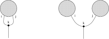
Figure 6: Contributions to $W_{1}^{(h)}$

The amplitudes shown in fig. 6 are uniquely connected by the loop equations to lower order terms given in fig. 7. (We select for the purpose of our argument a term with $k\neq i,j$ which does not give rise to short distance corrections at the extra vertex placed at $a_{k}$.)

Figure 7: Lower order amplitudes related to those of fig. 6

But for the latter amplitudes holds the inductive assumption and therefore also for all contributions to $\mathcal{F}^{(h)}$ which are not belonging to the local part $\widehat{\mathcal{F}}^{(h)}$ of $\mathcal{F}^{(h)}$. It is then in particular true that the local vertices making up $\mathcal{F}^{(h)}$ are those which were already present in $\mathcal{F}^{(h-1)}$ (covered by the inductive assumption) and the new local vertex for $\widehat{\mathcal{F}}^{(h)}$ (and then also for $\widehat{W}_{1}^{(h)},\mathcal{L}_{2}^{(h)},$ etc.). This concludes the argument.
The missing part for a full proof of the above theorem, that is, a control of symmetry numbers in 2 loop order and beyond, requires a detailed combinatorical analysis and will be given in a separate forthcoming publication [19].

5 Summary and conclusions

The purpose of the paper was to develop a Lagrangean formalism of Hermitean 1-matrix models taking as starting point Eynard’s technique [4] encoded in the hyperelliptic Riemann surface associated as spectral surface to the matrix model. Eynard’s approach is based on 2 ingredients: 1.) The differential 1-form attached to the defining equation of the hyperelliptic surface and 2.) the two-differential, the Bergmann kernel, on the reduced surface. Those ingredients are found to show up in the solution of the loop equations for the connected correlation function of resolvent operators given by an iterative nested system of Cauchy contour integrals. We resolved this nested system into the rules for an effective Lagrange of a scalar field propagating on the reduced surface, s.t. the propagation is by the Bergmann kernel with multiple self-interactions of the scalar field taking place at the branch points. The interactions are represented as a formal infinite power series in powers of the scalar fields and its derivatives and are subject to short distance corrections—due to the singularity of the Bergmann kernel at coinciding points—at all orders of the topological expansion. Our motivation for the endeavour to construct a Lagrange formalism is to find a new approach to critical behaviour via the renormalization group. The test of the usefulness of the formalism in this context is still ahead of us.
Evidently, the formalism reveals an abundantly rich true Lagrangean structure behind Eynard’s trivalent graphical representation.

References

• [1] E. Brezin, C. Itzykson, G. Parisi and J.B. Zuber, Planar Diagrams, Comm. Math. Phys. 59 (1978) 35
• [2] P. Di Francesco, P. Ginsparg and J. Zinn-Justin, 2D gravity and random matrices, Phys. Rept. 254 (1995) 1
• [3] G. Akemann, Higher genus correlators for the hermitian matrix model with multiple cuts, Nucl. Phys. B482 (1996) 403
• [4] B. Eynard, Topological expansion for the 1-hermitian matrix model correlation functions, JHEP 0411 (2004) 031
• [5] L. Chekhov and B. Eynard, Hermitian matrix model free energy: Feynman graph technique for all genera, JHEP 0603 (2006) 014
• [6] B. Eynard, Large N expansion of the 2-matrix model, multicut case, arXiv:math-ph/0307052
• [7] B. Eynard and N. Orantin, Topological expansion of the 2-matrix model correlation functions: diagrammatic rules for a residue formula, JHEP 0512 (2005) 034
• [8] B. Eynard and N. Orantin, Invariants of algebraic curves and topological expansion, arXiv:math-ph/0702045
• [9] M. Kontsevich, Intersection theory on the moduli space of curves and the matrix Airy function, Comm. Math. Phys. 147 (1992) 1
• [10] M. Mari$\tilde{\rm n}$o, Open string amplitudes and large order behavior in topological string theories, JHEP 0803 (2008) 060
• [11] B. Eynard, M. Mari$\tilde{\rm n}$o and N. Orantin, Holomorphic anomaly and matrix models, JHEP 0706 (2007) 058
• [12] V. Bouchard, A. Klemm, M. Mari$\tilde{\rm n}$o and Sara Pasquetti, Remodeling the B-model, arXiv:0709.1453 [hep-th]
• [13] R. Dijkgraaf and C. Vafa, Two Dimensional Kodaira-Spencer Theory and Three Dimensional Chern-Simons Gravity, arXiv:0711.1932 [hep-th]
• [14] B. Eynard and N. Orantin, Weil-Petersson volume of moduli spaces, Mirzakhani’s recursion and matrix models, arXiv:0705.3600 [math-ph]
• [15] B. Eynard, Recursion between Mumford volumes of moduli spaces, arXiv:0706.4403 [math.AG]
• [16] V. Bouchard and M. Mari$\tilde{\rm n}$o, Hurwitz numbers, matrix models and enumerative geometry, arXiv:0709.1458 [math.AG]
• [17] L. Chekhov, A. Marshakov, A. Mironov and D. Vasiliev, Complex Geometry of Matrix Models, arXiv:hep-th/0506075
• [18] H.E. Rauch, Weierstrass points, branch points, and moduli of Riemann sufaces, Comm. Pure Appl. Math. 12 (1959) 543
• [19] J. Grossehelweg, Rechnungen am 1-Matrixmodell, diploma thesis, Bonn IB-2006-12 (2006)
• [20] A. Klitz, in preparation
• [21] L. Chekhov, Genus one correlation to multi-cut matrix model solutions, Theor. Math. Phys. 141 (2004) 1640