NNLO QCD contributions to the flavor nonsinglet sector of
Abstract
We present the results of our QCD analysis for nonsinglet unpolarized quark distributions and structure function . New parameterizations are derived for the nonsinglet quark distributions for the kinematic wide range of and . The analysis is based on the Jacobi polynomials expansion of the structure function. The higher twist contributions of proton and deuteron structure function are obtained in the large region. Our calculations for nonsinglet unpolarized quark distribution functions based on the Jacobi polynomials method are in good agreement with the other theoretical models. The values of and are determined.
pacs:
13.60.Hb, 12.39.-x, 14.65.BtI Introduction
The deep-inelastic lepton-nucleon scattering is the source of important information about the nucleons structure. New and very precise data on nucleon structure functions have had a profound impact on our knowledge of parton distributions, in the small and large region. During the last years the accuracy of the obtained experimental data has extensively grown up enough to study in detail the status of the comparison of the available data with the theoretical predictions of quantum chromodynamics (QCD) in the different regions of momentum transfer.
The importance of deep-inelastic scattering (DIS) for QCD goes well beyond the measurement of Altarelli:2008fd . In the past it played a crucial role in establishing the reality of quarks and gluons as partons and in promoting QCD as the theory of strong interactions. Nowadays it still generates challenges to QCD as, for example, in the domain of structure functions at small Altarelli:2008aj ; Altarelli:2008xp or of polarized structure functions Atashbar Tehrani:2007be or of generalized parton densities Khorramian:2006wg and so on.
All calculations of high energy processes with initial hadrons, whether within the standard model or exploring new physics, require parton distribution functions (PDF’s) as an essential input. The reliability of these calculations, which underpins both future theoretical and experimental progress, depends on understanding the uncertainties of the PDF’s. The assessment of PDF’s, their uncertainties and extrapolation to the kinematics relevant for future colliders such as the LHC is an important challenge to high energy physics in recent years.
The PDF’s are derived from global analysis of experimental data from a wide range of hard processes in the framework of perturbative QCD. In this work this important problem is studied with the help of the method of the structure function reconstruction over their Mellin moments, which is based on the expansion of the structure function in terms of Jacobi polynomials. This method was developed and applied for QCD analysis parisi ; Barker ; Krivokhizhin:1987rz ; Krivokhizhin:1990ct ; Chyla:1986eb ; Barker:1980wu ; Kataev:1997nc ; Kataev:1998ce ; Kataev:1999bp ; Kataev:2001kk ; Khorramian:2007zz . The same method has also been applied in polarized case in Refs. Leader:1997kw and Atashbar Tehrani:2007be ; Khorramian:2007gu ; Khorramian:2007zza ; Mirjalili:2007ep ; Mirjalili:2006hf .
In this paper we use the deep-inelastic world data for nonsinglet QCD analysis to obtain the parton distribution function up to next-to-next-to-leading order (NNLO) approximations. The results of the present analysis is based on the Jacobi polynomials expansion of the nonsinglet structure function.
The plan of the paper is to give an introduction of the Jacobi polynomials approach in Sec. II. The method of the QCD analysis of nonsinglet structure function, based on Jacobi polynomials are written down in this section. In Section III we present a brief review of the theoretical formalism of the QCD analysis. A description of the procedure of the QCD fit of data are illustrated in Sec. IV. Section V contains final results of the QCD analysis. Our conclusions are summarized in Sec. VI.
II Jacobi polynomials approach
The evolution equations allow one to calculate the -dependence of the parton distributions provided at a certain reference point . These distributions are usually parameterized on the basis of plausible theoretical assumptions concerning their behavior near the end points .
One of the simplest and fastest possibilities in the structure function reconstruction from the QCD predictions for its Mellin moments is Jacobi polynomials expansion. The Jacobi polynomials are especially suitable for this purpose since they allow one to factor out an essential part of the -dependence of the structure function into the weight function parisi . Thus, given the Jacobi moments , a structure function may be reconstructed in a form of the series Barker ; Krivokhizhin:1987rz ; Krivokhizhin:1990ct ; Chyla:1986eb ; Barker:1980wu
| (1) |
where is the number of polynomials and are the Jacobi polynomials of order ,
| (2) |
where are the coefficients expressed through functions and satisfy the orthogonality relation with the weight as in the following:
| (3) |
For the moment, we note that the dependence is entirely contained in the Jacobi moments
| (4) | |||||
obtained by inverting Eq. (1), using Eqs. (2,
3) and also definition of moments,
.
Using Eqs. (1-4) now, one can relate the
structure function with its Mellin moments
| (5) | |||||
where are the moments determined in the next section. , and have to be chosen so as to achieve the fastest convergence of the series on the right-hand side of Eq. (5) and to reconstruct with the required accuracy. In our analysis we use , and . The same method has been applied to calculate the nonsinglet structure function from their moments Kataev:1997nc ; Kataev:1998ce ; Kataev:1999bp ; Kataev:2001kk and for polarized structure function Atashbar Tehrani:2007be ; Leader:1997kw ; Khorramian:2007gu .
Obviously the -dependence of the polarized structure function is defined by the -dependence of the moments.
III Theoretical formalism of the QCD analysis
In the common factorization scheme the relevant structure function as extracted from the DIS process can be, up to NNLO, written as ref3 ; ref4 ; ref5 ; Gluck:2006pm
| (6) |
The nonsinglet structure function for three active (light) flavors has the representation
| (7) | |||||
The flavor singlet and gluon contributions in Eq. (6) reads
| (8) | |||||
| (9) | |||||
The symbol denotes the Mellin convolution
| (10) |
In Eq. (7) and , where . Also in Eq. (8) . Notice that in the above equations denotes the strong coupling constant and are the Wilson coefficients Vermaseren:2005qc .
The combinations of parton densities in the nonsinglet regime and the valence region for in LO is
| (11) |
where , and , since sea quarks can be neglected in the region . So in the -space we have
| (12) |
In the above region the combinations of parton densities for are also given by
| (13) |
where and .
In the region for the difference of the proton and deuteron data we use
| (14) | |||||
where now since sea quarks cannot be neglected for smaller than about 0.3. In our calculation we supposed the distribution
| (15) |
at GeV2 which gives a good description of the Drell-Yan dimuon production data E866 . In our analysis we used the above distribution for considering the symmetry breaking of sea quarks ref19 ; Blumlein:2004pr . By using the solution of the nonsinglet evolution equation for the parton densities to 3 loop order Blumlein:2006be , the nonsinglet structure functions are given by
| (16) | |||||
Here and denotes the three above cases, i.e. proton, deuteron and nonsinglet structure function. are the nonsinglet Wilson coefficients in which can be found in FP ; NS2 ; Vermaseren:2005qc and denote also the Mellin transforms of the loop splitting functions.
The strong coupling constant plays a more central role in the present paper to the evolution of parton densities. At the scale dependence of is given by
| (17) |
The expansion coefficients of the -function of QCD are known up to , i.e., N2LO Tarasov:1980au ; Larin:1993tp
| (18) |
here stands for the number of effectively massless quark flavors. The strong coupling constant up to NNLO is as followings Vogt:2004ns :
| (19) |
where , , and is the QCD scale parameter.
IV The Procedure of the QCD Fits of Data
In the present analysis we choose the following parametrization for the valence quark densities
| (20) |
in the input scale of GeV2 and the normalizations and being fixed by and , respectively. By QCD fits of the world data for , we can extract valence quark densities using the Jacobi polynomials method. For the nonsinglet QCD analysis presented in this paper we use the structure function data measured in charged lepton proton and deuteron deep-inelastic scattering. The experiments contributing to the statistics are BCDMS BCDMS , SLAC SLAC , NMC NMC , H1 H1 , and ZEUS ZEUS . In our QCD analysis we use three data samples : , in the nonsinglet regime and the valence quark region and in the region .
The valence quark region may be parameterized by the nonsinglet combinations of parton distributions, which are expressed through the parton distributions of valence quarks. Only data with were included in the analysis and a cut in the hadronic mass of was applied in order to widely eliminate higher twist (HT) effects from the data samples. After these cuts we are left with 762 data points, 322 for , 232 for , and 208 for . By considering the additional cuts on the BCDMS () and on the NMC data( GeV2) the total number of data points available for the analysis reduce from 762 to 551.
The simplest possible choice for the function would be
| (21) |
where is the error associated with data point . Through , is a function of the theory parameters. Minimization of would identify parameter values for which the theory fits the data. However, the simple form is appropriate only for the ideal case of a uniform data set with uncorrelated errors. For data used in the global analysis, most experiments combine various systematic errors into one effective error for each data point, along with the statistical error. Then, in addition, the fully correlated normalization error of the experiment is usually specified separately. For this reason, it is natural to adopt the following definition for the effective Stump:2001gu :
| (22) | |||||
| (23) |
For the experiment, , , and denote the data value, measurement uncertainty (statistical and systematic combined), and theoretical value for the data point. is the experimental normalization uncertainty and is an overall normalization factor for the data of experiment . The factor is a possible weighting factor(with default value). However, we allowed for a relative normalization shift between the different data sets within the normalization uncertainties quoted by the experiments. For example the normalization uncertainty of the NMC(combined) data is estimated to be 2.5%. The normalization shifts were fitted once and then kept fixed.
The number of data points for the nonsinglet QCD analysis with their and ranges, and the normalization shifts determined are summarized in Table. I. In this table the first column gives (in parentheses) the beam momentum in GeV of the respective data set (number), a flag whether the data come from a combined analysis of all beam momenta (comb) or whether the data are taken at high momentum transfer (hQ2). The and range indicate in the second and third columns, respectively. The fourth column () contains the number of data points according to the cuts: , , for and and for . The reduction of the number of data points by the additional cuts on the BCDMS data () and on the NMC data () are given in the fifth column (). The last column () contains the normalization shifts.
Now the sums in run over all data sets and in each data set over all data points. The minimization of the above value to determine the best parametrization of the unpolarized parton distributions is done using the program MINUIT MINUIT .
| Experiment | |||||
|---|---|---|---|---|---|
| BCDMS (100) | 0.35 – 0.75 | 11.75 – 75.00 | 51 | 29 | 1.005 |
| BCDMS (120) | 0.35 – 0.75 | 13.25 – 75.00 | 59 | 32 | 0.998 |
| BCDMS (200) | 0.35 – 0.75 | 32.50 – 137.50 | 50 | 28 | 0.998 |
| BCDMS (280) | 0.35 – 0.75 | 43.00 – 230.00 | 49 | 26 | 0.998 |
| NMC (comb) | 0.35 – 0.50 | 7.00 – 65.00 | 15 | 14 | 1.000 |
| SLAC (comb) | 0.30 – 0.62 | 7.30 – 21.39 | 57 | 57 | 1.013 |
| H1 (hQ2) | 0.40 – 0.65 | 200 – 30000 | 26 | 26 | 1.020 |
| ZEUS (hQ2) | 0.40 – 0.65 | 650 – 30000 | 15 | 15 | 1.007 |
| proton | 322 | 227 |
(a) Number of data points.
Experiment
BCDMS (120)
0.35 – 0.75
13.25 – 99.00
59
32
1.001
BCDMS (200)
0.35 – 0.75
32.50 – 137.50
50
28
0.998
BCDMS (280)
0.35 – 0.75
43.00 – 230.00
49
26
1.003
NMC (comb)
0.35 – 0.50
7.00 – 65.00
15
14
1.000
SLAC (comb)
0.30 – 0.62
10.00 – 21.40
59
59
0.990
deuteron
232
159
(b) Number of data points.
Experiment
BCDMS (120)
0.070 – 0.275
8.75 – 43.00
36
30
0.983
BCDMS (200)
0.070 – 0.275
17.00 – 75.00
29
28
0.999
BCDMS (280)
0.100 – 0.275
32.50 – 115.50
27
26
0.997
NMC (comb)
0.013 – 0.275
4.50 – 65.00
88
53
1.000
SLAC (comb)
0.153 – 0.293
4.18 – 5.50
28
28
0.994
nonsinglet
208
165
(c) Number of data
points.
The one error for the parton density as given by Gaussian error propagation is Blumlein:2006be
| (24) |
where the sum runs over all fitted parameters. The functions are the derivatives of with respect to the fit parameter , and are the elements of the covariance matrix. The derivatives can be calculated analytically at the input scale . Their values at are given by evolution which is performed in Mellin- space.
V Results
In the QCD analysis of the present paper we used three data sets: the structure functions and in the region of and the combination of these structure functions in the region of . Notice that we take into account the cuts GeV2, GeV2 for our QCD fits to determine some unknown parameters. In Fig.(1) the proton data for are shown in the nonsinglet regime and the valence quark region indicating the above cuts by a vertical dashed line. The solid lines correspond to the NNLO QCD fit.
Now, it is possible to take into account the target mass effects in our calculations. The perturbative form of the moments is derived under the assumption that the mass of the target hadron is zero (in the limit ). At intermediate and low this assumption will begin to break down and the moments will be subject to potentially significant power corrections, of order , where is the mass of the nucleon. These are known as target mass corrections (TMCs) and when included, the moments of flavor nonsinglet structure function have the form Georgi:1976ve ; Gluck:2006yz
| (25) | |||||
where higher powers than are negligible for the relevant region. By inserting Eq. (25) in Eq. (5) we have
| (26) |
where are the moments determined by Eq. (25). In Fig.(1) the dashed lines correspond to the NNLO QCD fit adding target mass corrections.
Despite the kinematic cuts ( GeV2, GeV2) used for our analysis, we also take into account higher twist corrections to and in the kinematic region in order to learn whether nonperturbative effects may still contaminate our perturbative analysis. For this purpose we extrapolate the QCD fit results obtained for to the region and form the difference between data and theory, applying target mass corrections in addition. Now by considering higher twist correction (HT)
| (27) |
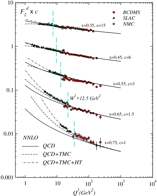
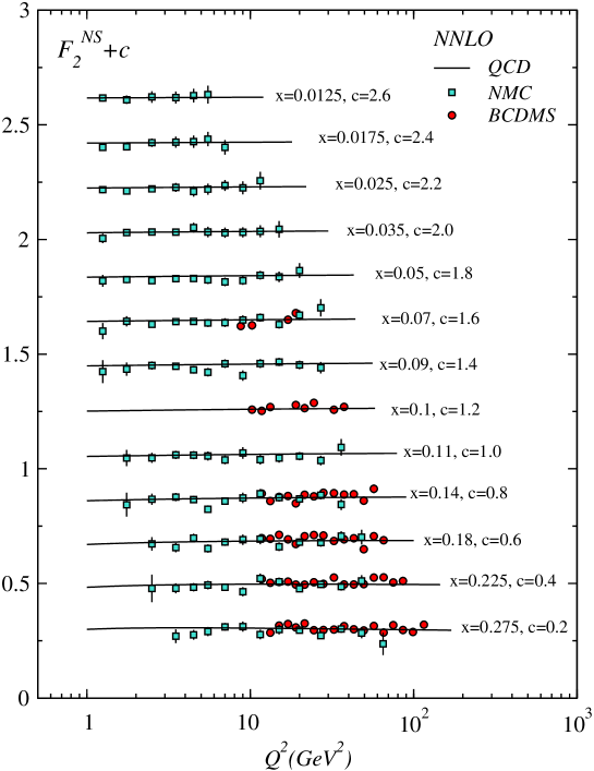
the higher twist coefficient can be extract. Here the operation denotes taking the target mass corrections of the twist–2 contributions to the respective structure function. The coefficients are determined in bins of and and are then averaged over . We extrapolate our QCD fits to the region in Fig.(1). The dashed-dotted lines in this figure correspond to the NNLO QCD fit adding target mass and higher twist corrections. There, at higher values of a clear gap between the data and the QCD fit is seen. Figure (2) shows the corresponding results for the deuteron data. Figure (3) shows the result of the pure QCD fit for the nonsinglet structure function in NNLO.
| LO | NLO | NNLO | ||
| 0.6698 0.0073 | 0.7434 0.009 | 0.7772 0.009 | ||
| 3.5104 0.042 | 3.8907 0.040 | 4.0034 0.033 | ||
| 0.1990 | 0.1620 | 0.1000 | ||
| 1.498 | 1.2100 | 1.1400 | ||
| 0.6850 0.035 | 0.7369 0.040 | 0.7858 0.043 | ||
| 3.1685 0.192 | 3.5051 0.225 | 3.6336 0.244 | ||
| 0.5399 | 0.3899 | 0.1838 | ||
| -1.4000 | -1.3700 | -1.2152 | ||
| , MeV | 213.2 28 | 263.8 30 | 239.9 27 | |
| 538/546 = 0.9853 | 523/546 = 0.9578 | 506/546 = 0.9267 | ||
| LO | |||||
|---|---|---|---|---|---|
| 5.2810-5 | |||||
| 1.6510-4 | 1.7310-3 | ||||
| -7.3910-5 | -4.5510-4 | 1.2310-3 | |||
| -2.6410-4 | -2.1210-3 | 6.1510-3 | 3.6710-2 | ||
| 1.9010-5 | -8.3410-4 | 2.3910-5 | -3.1610-4 | 7.7910-4 | |
| NLO | |||||
| 8.8710-5 | |||||
| 2.3910-4 | 1.6310-3 | ||||
| -1.3410-4 | -7.8610-4 | 1.6110-3 | |||
| -5.1010-4 | -4.1910-3 | 8.3310-3 | 5.0710-2 | ||
| 8.7110-5 | -5.3910-4 | 8.0910-5 | 2.5710-4 | 8.8010-4 | |
| NNLO | |||||
| 7.6110-5 | |||||
| 1.7310-4 | 1.1010-3 | ||||
| -8.4110-5 | -6.6210-4 | 1.8510-3 | |||
| -2.7310-4 | -3.7310-3 | 9.7910-3 | 5.9810-2 | ||
| 1.0810-4 | -2.7410-4 | 1.0610-4 | 4.1910-4 | 7.4110-4 |
In Table (2) we summarize the LO, NLO, and NNLO fit results without HT contributions for the parameters of the parton densities , and . The resulted value of is 0.9853 at LO, 0.9578 at NLO, and 0.9267 at NNLO. Our results for covariance matrix for LO, NLO, and NNLO are presented in Table(3).
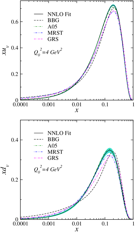
Figure (4) illustrates our fit results for , at at NNLO with correlated errors. We compare with the results of Blumlein:2006be ; Alekhin:2005gq ; Gluck:2006yz and a very recent analysis Martin:2007bv . Our results for and are in good agreement with the other theoretical model at the one level.
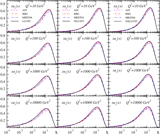
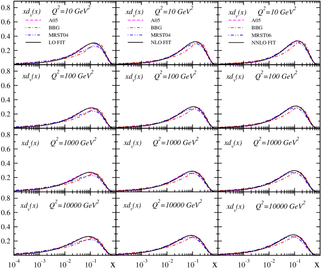
In Figs. (5) and (6) we show the evolution of the valence quark distributions and from to in the region up to NNLO. We also compared with other QCD analysis Alekhin:2005gq ; Blumlein:2006be ; Martin:2007bv ; MRST04 . With rising values of the distributions flatten at large values of and rise at low values.
Another way to compare the NNLO fit results consists in forming moments of the distributions and . In Table 4 we present the lowest non-trivial moments of these distributions at in NNLO and compare to the respective moments obtained for the parameterizations Blumlein:2006be ; MRST04 ; A02 ; Alekhin:2006zm .
| NNLO | BBG | MRST04 | A02 | A06 | ||
|---|---|---|---|---|---|---|
| 2 | 0.3056 0.0023 | 0.2986 0.0029 | 0.285 | 0.304 | 0.2947 | |
| 3 | 0.0871 0.0009 | 0.0871 0.0011 | 0.082 | 0.087 | 0.0843 | |
| 4 | 0.0330 0.0004 | 0.0333 0.0005 | 0.032 | 0.033 | 0.0319 | |
| 2 | 0.1235 0.0023 | 0.1239 0.0026 | 0.115 | 0.120 | 0.1129 | |
| 3 | 0.0298 0.0008 | 0.0315 0.0008 | 0.028 | 0.028 | 0.0275 | |
| 4 | 0.0098 0.0004 | 0.0105 0.0004 | 0.009 | 0.010 | 0.0092 |
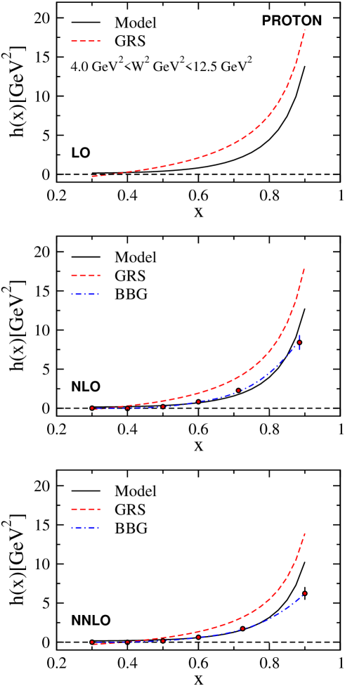
To perform higher twist QCD analysis of the nonsinglet world data up to NNLO, we consider the cuts. The number of data points in the above range for proton and deuteron is 279 and 278, respectively. The extracted distributions for up to NNLO are depicted in Fig.(7) for the nonsinglet case considering scattering off the proton target. According to our results the coefficient grows towards large . Also in this figure HT contributions have the tendency to decrease form LO to NLO, NNLO. This effect was observed for the first time in the case of fits of DIS data in Kataev:1997nc and then studied in more detail in Kataev:1999bp ; Kataev:2001kk .
This similar effect was also observed in the fits of charge lepton-nucleon DIS data Yang:1999xg ; Blumlein:2006be ; Gluck:2006yz ; Blumlein:2008kz . To compare, we also present the reported results of the early NNLO analysis Blumlein:2008kz ; Gluck:2006yz in Fig.(7). Note that the results for in LO are not presented in the BBG model Blumlein:2006be ; Blumlein:2008kz . In Ref. Gluck:2006yz , the functional form for is chosen by
| (28) |
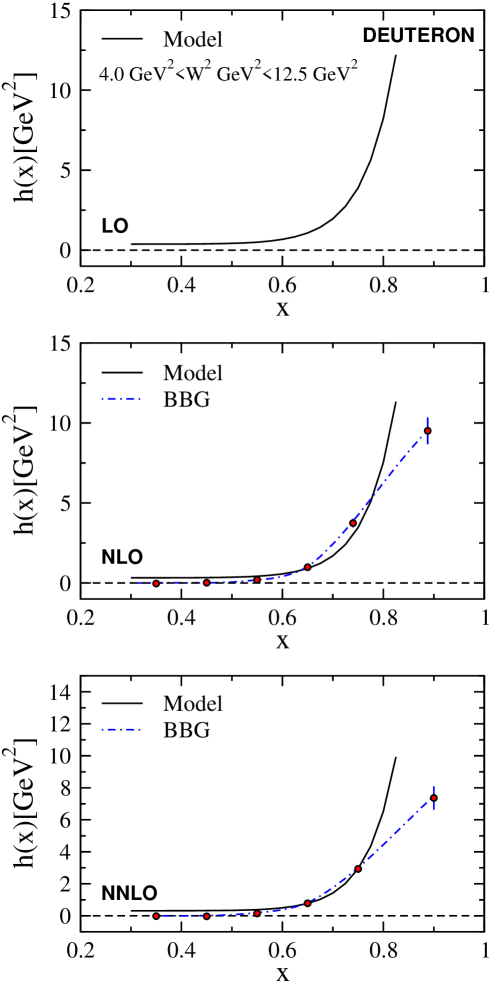
and it is possible to compare results even in LO. Fig.(8) shows our results for and for the deuteron target up to NNLO. Also we compare the results for the BBG model Blumlein:2008kz . The same as the proton, HT contributions for the deuteron have the tendency to decrease form LO to NLO, NNLO. As seen from Fig.(7) and Fig.(8) is widely independent of the target comparing the results for deeply inelastic scattering off protons and deuterons. Our results in low- are also in good agreement with Blumlein:2006be ; Blumlein:2008kz .
VI Discussion
We have performed a QCD analysis of the flavor nonsinglet unpolarized deep–inelastic charged lepton–nucleon scattering data to next–to–leading order and derived parameterizations of valence quark distributions at a starting scale together with the QCD–scale by using the Jacobi polynomial expansions.
The analysis was performed using the Jacobi polynomials–method to determine the parameters of the problem in a fit to the data. A new aspect in comparison with previous analysis is that we determine the parton densities and the QCD scale up to NNLO by using the Jacobi polynomial expansion method. The benefit of this approach is the possibility to determine nonsinglet parton distributions analytically and not numerically. In Ref. Program:summary we arrange the MATHEMATICA program to extract and .
In this paper the flavor asymmetric combination of light parton distributions of Eq. (15) are fixed at 4 GeV2, as GRS Gluck:2006yz and BBG Blumlein:2004pr ; Blumlein:2006be applied, and gives a good description of the Drell-Yan dimuon production data Towell:2001nh . The first clear evidence for the flavor asymmetry of the nucleon sea in nature came from the analysis of NMC at CERN Amaudruz:1991at . In order to have the link with NMC data, we want to study the compatibility of the with the NMC result for the Gottfried sum rule (GSR)Gottfried:1967kk . This sum rule is still actively discussed in problems of deep-inelastic scattering. The GSR, , can be expressed in terms of the parton distribution functions as
| (29) | |||||
In the derivation of the above equation, the asymmetry of nucleon sea was assumed. The NMC measurement Amaudruz:1991at implies at GeV2
| (30) |
which was the first indication that there are more down antiquarks in the proton than up antiquarks. On the other hand this value is reported at GeV2 E866 . Now it is interesting to obtain this value for the parametrization of Eq. (15) which we used in our QCD analysis. By integration of this distribution we obtain which is smaller than the reported results in the literature. However, the NMC Collaboration gives the experimental value at GeV2 Amaudruz:1991at
| (31) |
By using Eq. (29) we obtain the GSR value about 0.267 with which the existing measurements are almost compatible within error. It seems that although the value of is smaller than the values in the literature, the parametrization of Eq. (15) can give a good description of the E866 experimental data E866 . Also we should notice that the GSR does not belong to the strict sum rules in QCD and it is necessary to receive not only QCD corrections but anomalous dimensions as well Kataev:2007jz ; Kataev:2003en ; Kataev:2003xp ; Broadhurst:2004jx ; Broadhurst:2004kh ; Kataev:2004wv .
Now it is interesting to compare the NNLO theoretical QCD theoretical prediction for the Gottfried sum rule Broadhurst:2004jx with NMC data. The recent step in this direction was done in Abbate:2005ct . According to this paper we add the QCD two-loop correction to the Gottfried sum rule and we refine the GSR value to about . Also we obtain the value of which is well compatible with the neural parametrization results, e.g. Abbate:2005ct within errors.
In the QCD analysis we parameterized the strong coupling constant in terms of four massless flavors determining . The LO, NLO, and NNLO results fitting the data, are
| (32) |
These results can be expressed in terms of :
| (33) |
Note that in above results we use the matching between and flavor couplings calculated in Ref. Chetyrkin:1997sg . To be capable to compare with other measurement of we adopt this prescription.
The values can be compared with results from other QCD analysis of inclusive deep–inelastic scattering data in NLO
| A02 A02 : | =0.1171 | 0.0015 | ||
|---|---|---|---|---|
| ZEUS ZEUS_Ch : | =0.1166 | 0.0049 | ||
| H1 H1 : | =0.1150 | 0.0017 | ||
| BCDMS BCDMS : | =0.110 | 0.006 | ||
| GRS Gluck:2006yz : | =0.112 | |||
| CTEQ6 CTEQ_P : | =0.1165 | 0.0065 | ||
| MRST03 MRST03 : | =0.1165 | 0.0020 | ||
| BBG Blumlein:2006be : | =0.1148 | 0.0019 | ||
| KK05 Krivokhizhin:2005pt : | =0.1153 | 0.0013() | ||
| 0.0022() 0.0012() | ||||
| BB (pol)BB02 : | =0.113 | 0.004 | ||
| AK (pol) Atashbar Tehrani:2007be : | =0.1141 | 0.0036 |
The NNLO values of can also be compared with results from other QCD analysis
| A02 A02 : | =0.1143 | 0.0014 | ||
|---|---|---|---|---|
| GRS Gluck:2006yz : | =0.111 | |||
| MRST03 MRST03 : | = 0.1153 | 0.0020 | ||
| SY01(ep) SY : | =0.1166 | 0.0013 | ||
| SY01(N) SY : | =0.1153 | 0.0063 | ||
| A06 Alekhin:2006zm : | =0.1128 | 0.0015 | ||
| BBG Blumlein:2006be : | =0.1134 | |||
| BM07 Brooks:2006wh : | =0.1189 | 0.0019 | ||
| KPS00() Kataev:1999bp : | =0.118 | 0.002 () 0.005 () | ||
| 0.003 () | ||||
| KPS03() Kataev:2001kk : | =0.119 | 0.002 () 0.005 () | ||
| 0.002 () () |
and with the value of the current world average
| (34) |
which has been extracted in Bethke:2006ac recently.
We hope our results of QCD analysis of structure functions in terms of Jacobi polynomials could be able to describe more complicated hadron structure functions. We also hope to be able to consider the N3LO corrections and massive quark contributions by using the structure function expansion in terms of the Jacobi polynomials.
Acknowledgements.
We are especially grateful to G. Altarelli and J. Blümlein for guidance and critical remarks. A.N.K. is grateful to S. Albino for useful discussions. We would like to thank M. Ghominejad and Z. Karamloo for reading the manuscript of this paper. A.N.K. thanks Semnan University for partial financial support of this project. We acknowledge the Institute for Studies in Theoretical Physics and Mathematics (IPM) for financially supporting this project.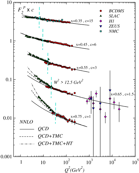
References
- (1) G. Altarelli, arXiv:0804.4147 [hep-ph].
- (2) G. Altarelli, R. D. Ball and S. Forte, Nucl. Phys. B 799, 199 (2008) [arXiv:0802.0032 [hep-ph]].
- (3) G. Altarelli, R. D. Ball and S. Forte, PoS RADCOR2007, 028 (2007) [arXiv:0802.0968 [hep-ph]].
- (4) S. Atashbar Tehrani and A. N. Khorramian, JHEP 0707, 048 (2007) [arXiv:0705.2647 [hep-ph]].
- (5) A. N. Khorramian and S. Atashbar Tehrani, JHEP 0703, 051 (2007) [arXiv:hep-ph/0610136].
-
(6)
G. Parisi and N. Sourlas,
Nucl. Phys. B151 (1979) 421;
I. S. Barker, C. B. Langensiepen and G. Shaw, Nucl. Phys. B186 (1981) 61. -
(7)
I. S. Barker, B. R. Martin and G. Shaw,
Z. Phys. C19 (1983) 147;
I. S. Barker and B. R. Martin, Z. Phys. C24 (1984) 255;
S. P. Kurlovich, A. V. Sidorov and N. B. Skachkov, JINR Report E2-89-655, Dubna, 1989. - (8) V. G. Krivokhizhin, S. P. Kurlovich, V. V. Sanadze, I. A. Savin, A. V. Sidorov and N. B. Skachkov, Z. Phys. C 36 (1987) 51.
- (9) V. G. Krivokhizhin et al., Z. Phys. C 48, 347 (1990).
- (10) J. Chyla and J. Rames, Z. Phys. C 31 (1986) 151.
- (11) I. S. Barker, C. S. Langensiepen and G. Shaw, Nucl. Phys. B 186 (1981) 61.
- (12) A. L. Kataev, A. V. Kotikov, G. Parente and A. V. Sidorov, Phys. Lett. B 417, (1998) 374 [arXiv:hep-ph/9706534].
- (13) A. L. Kataev, G. Parente and A. V. Sidorov, arXiv:hep-ph/9809500.
- (14) A. L. Kataev, G. Parente and A. V. Sidorov, Nucl. Phys. B 573, (2000) 405 [arXiv:hep-ph/9905310].
-
(15)
A. L. Kataev, G. Parente and A. V. Sidorov,
Phys. Part. Nucl. 34, (2003) 20
[arXiv:hep-ph/0106221];
A. L. Kataev, G. Parente and A. V. Sidorov, Nucl. Phys. Proc. Suppl. 116 (2003) 105 [arXiv:hep-ph/0211151]. - (16) A. N. Khorramian, S. A. Tehrani and M. Ghominejad, Acta Phys. Polon. B 38, 3551 (2007).
- (17) E. Leader, A. V. Sidorov and D. B. Stamenov, Int. J. Mod. Phys. A 13, 5573 (1998) [arXiv:hep-ph/9708335].
- (18) A. N. Khorramian and S. A. Tehrani, arXiv:0712.2373 [hep-ph].
- (19) A. N. Khorramian and S. Atashbar Tehrani, AIP Conf. Proc. 915, 420 (2007).
- (20) A. Mirjalili, A. N. Khorramian and S. Atashbar-Tehrani, Nucl. Phys. Proc. Suppl. 164, 38 (2007).
- (21) A. Mirjalili, S. Atashbar Tehrani and A. N. Khorramian, Int. J. Mod. Phys. A 21, 4599 (2006) [arXiv:hep-ph/0608224].
- (22) W.L. van Neerven, A. Vogt, Nucl. Phys. B568, 263 (2000)
- (23) W.L. van Neerven, A. Vogt, Nucl. Phys. B588, 345 (2000) and arXiv:hep-ph/0006154 (corrected)
- (24) J. Blümlein, A. Vogt, Phys. Rev. D58, 014020 (1998).
- (25) M. Gluck, C. Pisano and E. Reya, Eur. Phys. J. C 50, 29 (2007) [arXiv:hep-ph/0610060].
- (26) J. A. M. Vermaseren, A. Vogt and S. Moch, Nucl. Phys. B 724 (2005) 3 [arXiv:hep-ph/0504242].
- (27) R.S. Towell et al., E866 Collab., Phys. Rev. D64 (2001) 052002.
- (28) A.D. Martin et al., Eur. Phys. J. C23 (2002) 73.
- (29) J. Blümlein, H, Böttcher, and A. Guffanti, Nucl. Phys. B (Proc. Suppl.) 135 (2004) 152.
- (30) J. Blumlein, H. Bottcher and A. Guffanti, Nucl. Phys. B 774, 182 (2007) [arXiv:hep-ph/0607200].
- (31) W. Furmanski and R. Petronzio, Z. Phys. C 11 (1982) 293.
-
(32)
W. L. van Neerven and E. B. Zijlstra,
Phys. Lett. B 272 (1991) 127;
E. B. Zijlstra and W. L. van Neerven, Nucl. Phys. B 383 (1992) 525. - (33) O. V. Tarasov, A. A. Vladimirov and A. Y. Zharkov, Phys. Lett. B 93, 429 (1980).
- (34) S. A. Larin and J. A. M. Vermaseren, Phys. Lett. B 303, 334 (1993) [arXiv:hep-ph/9302208].
- (35) A. Vogt, Comput. Phys. Commun. 170, 65 (2005) [arXiv:hep-ph/0408244].
-
(36)
A.C. Benvenuti et al. [BCDMS Collaboration],
Phys. Lett. B 237 (1990) 592;
A.C. Benvenuti et al. [BCDMS Collaboration], Phys. Lett. B223 (1989) 485; Phys. Lett. B237 (1990) 592.
A.C. Benvenuti et al. [BCDMS Collaboration], Phys. Lett. B 237 (1990) 599. - (37) L. W. Whitlow, E. M. Riordan, S. Dasu, S. Rock and A. Bodek, Phys. Lett. B 282 (1992).
- (38) M. Arneodo et al. [New Muon Collaboration], Nucl. Phys. B 483 (1997) 3 [arXiv:hep-ph/9610231].
-
(39)
C. Adloff et al. [H1 Collaboration],
Eur. Phys. J. C 21 (2001) 33
[arXiv:hep-ex/0012053];
C. Adloff et al. [H1 Collaboration], Eur. Phys. J. C 30 (2003) 1 [arXiv:hep-ex/0304003]. -
(40)
J. Breitweg et al. [ZEUS Collaboration],
Eur. Phys. J. C 7 (1999) 609
[arXiv:hep-ex/9809005];
S. Chekanov et al. [ZEUS Collaboration], Eur. Phys. J. C 21 (2001) 443 [arXiv:hep-ex/0105090]. - (41) D. Stump et al., Phys. Rev. D 65, 014012 (2002) [arXiv:hep-ph/0101051].
- (42) F. James, CERN Program Library, Long Writeup D506 (MINUIT).
- (43) H. Georgi and H. D. Politzer, Phys. Rev. D 14 (1976) 1829.
- (44) M. Gluck, E. Reya and C. Schuck, Nucl. Phys. B 754, 178 (2006) [arXiv:hep-ph/0604116].
- (45) S. Alekhin, JETP Lett. 82, 628 (2005) [Pisma Zh. Eksp. Teor. Fiz. 82, 710 (2005)] [arXiv:hep-ph/0508248].
- (46) A. D. Martin, W. J. Stirling, R. S. Thorne and G. Watt, Phys. Lett. B 652, 292 (2007) [arXiv:0706.0459 [hep-ph]].
- (47) A. D. Martin, R. G. Roberts, W. J. Stirling and R. S. Thorne, Phys. Lett. B 604 (2004) 61 [arXiv:hep-ph/0410230].
- (48) S. Alekhin, Phys. Rev. D 68 (2003) 014002 [arXiv:hep-ph/0211096].
- (49) S. Alekhin, K. Melnikov and F. Petriello, Phys. Rev. D 74, 054033 (2006) [arXiv:hep-ph/0606237].
- (50) U. K. Yang and A. Bodek, Eur. Phys. J. C 13, 241 (2000) [arXiv:hep-ex/9908058].
- (51) J. Blumlein and H. Bottcher, Phys. Lett. B 662, 336 (2008) [arXiv:0802.0408 [hep-ph]].
- (52) Program summary URL: http://particles.ipm.ir/QCD.htm.
- (53) R. S. Towell et al. [FNAL E866/NuSea Collaboration], Phys. Rev. D 64, 052002 (2001) [arXiv:hep-ex/0103030].
- (54) P. Amaudruz et al. [New Muon Collaboration], Phys. Rev. Lett. 66, 2712 (1991); M. Arneodo et al. [New Muon Collaboration], Phys. Rev. D 50, 1 (1994); M. Arneodo et al. [New Muon Collaboration], Nucl. Phys. B 487, 3 (1997) [arXiv:hep-ex/9611022].
- (55) K. Gottfried, Phys. Rev. Lett. 18 (1967) 1174.
- (56) A. L. Kataev and G. Parente, Phys. Lett. B 566, 120 (2003) [arXiv:hep-ph/0304072].
- (57) A. L. Kataev, arXiv:hep-ph/0311091.
- (58) D. J. Broadhurst, A. L. Kataev and C. J. Maxwell, Phys. Lett. B 590, 76 (2004) [arXiv:hep-ph/0403037].
- (59) D. J. Broadhurst, A. L. Kataev and C. J. Maxwell, arXiv:hep-ph/0410058.
- (60) A. L. Kataev, Phys. Part. Nucl. 36, S168 (2005) [arXiv:hep-ph/0412369].
- (61) A. L. Kataev, PoS A CAT2007, 072 (2007) [arXiv:0707.2855 [hep-ph]].
- (62) R. Abbate and S. Forte, Phys. Rev. D 72, 117503 (2005) [arXiv:hep-ph/0511231].
- (63) K. G. Chetyrkin, B. A. Kniehl and M. Steinhauser, , Phys. Rev. Lett. 79 (1997) 2184 [arXiv:hep-ph/9706430]; S. Bethke, , J. Phys. G 26 (2000) R27 [arXiv:hep-ex/0004021]; W. Bernreuther and W. Wetzel, Nucl. Phys. B 197, 228 (1982) [Erratum-ibid. B 513, 758 (1998)].
- (64) S. Chekanov et al. [ZEUS Collaboration], Phys. Rev. D 67 (2003) 012007 [arXiv:hep-ex/0208023].
- (65) J. Pumplin, D. R. Stump, J. Huston, H. L. Lai, P. Nadolsky and W. K. Tung, JHEP 0207 (2002) 012 [arXiv:hep-ph/0201195].
- (66) A. D. Martin, R. G. Roberts, W. J. Stirling and R. S. Thorne, arXiv:hep-ph/0307262.
- (67) V. G. Krivokhizhin and A. V. Kotikov, Phys. Atom. Nucl. 68, 1873 (2005) [Yad. Fiz. 68, 1935 (2005)];
- (68) J. Blümlein and H. Böttcher, Nucl. Phys. B 636 (2002) 225 [arXiv:hep-ph/0203155].
- (69) J. Santiago and F. J. Yndurain, Nucl. Phys. B 611 (2001) 447 [arXiv:hep-ph/0102247].
- (70) P. M. Brooks and C. J. Maxwell, Nucl. Phys. B 780, 76 (2007) [arXiv:hep-ph/0610137].
- (71) S. Bethke, Prog. Part. Nucl. Phys. 58, 351 (2007) [arXiv:hep-ex/0606035].