Diffusion conductivity and weak localization in two-dimensional structures with electrostatically induced random antidots array

Abstract

Results of experimental study of the weak localization phenomenon in 2D system with artificial inhomogeneity of potential relief are presented. It is shown that the shape of the magnetoconductivity curve is determined by the statistics of closed paths. The area distribution function of closed paths has been obtained using the Fourier transformation of the magnetoconductivity curves taken at different temperatures. The experimental results are found in a qualitative agreement with the results of computer simulation.

The transport properties of the semiconductor two-dimensional (2D) structures with antidots array were intensively studied both experimentallyexper ; exper0 ; exper1 ; exper2 ; exper3 ; exper4 ; exper5 ; exper6 ; exper7 ; exper8 ; exper9 and theoreticallyTheory ; Theory0 ; Theory1 ; Theory2 ; Theory3 in last 10–15 years. The main concern was with the investigations of the ballistic systems, in which $l>d,\,D$, where $l$ is the mean free path, $d$ and $D$ are the size of antidots and period of the antidots array, respectively. The rich diversity of the transport phenomena, such as commensurable oscillations, the peculiarities due to the trajectories rolling along the array of antidots was observed. The antidots array structures in the diffusion regime ($l<d,D$) were not studied essentially. Such structures are interesting in some aspects. First of all, the quantum corrections to the conductivity due to weak localization (WL) and electron-electron (e-e) interaction have to reveal the specific features when the phase breaking length, $L_{\phi}=\sqrt{{\cal D}\tau_{\phi}}$, where ${\cal D}$ is the diffusion coefficient and $\tau_{\phi}$ is phase breaking time, or the temperature length, $L_{T}=\sqrt{{\cal D}/T}$, become larger than $d,D$ at decreasing temperature (hereafter we set $k_{B}=1$, $\hbar=1$). Secondly, the large enough negative gate voltage has to deplete the channels between the antidots (the channel width $w_{0}$ is about $D-d$) and as a result to lead to crossover to the hopping conductivity. Besides, from the transport properties standpoint the antidots arrays are the fine model of the granular media. In contrast to the granular metallic film, the parameters of the “granules” and “barriers” are reliably known and can be changed continuously within wide range.

In this paper we report the results of the experimental study of the weak localization correction to the conductivity in the structure with the random array of antidots. We show that the change of the magnetoresistance at arising of the antidots and increase of the antidots size results from the change of statistics of closed paths. Namely, the contribution of the trajectories with the large enclosed area is strongly suppressed. The experimental area distribution function is in a reasonable agreement with the function obtained from the computer simulation.

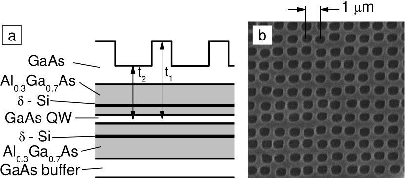
Figure 1: The sketch (a) and electron microscope image (b) of the structure investigated.

The random antidots array was made on the single quantum well heterostructure with the electron density $n=1.5\times 10^{12}$ cm^-2 and mobility $\mu=19000$ cm²/(V s) grown by the molecular beam epitaxy. It consists of a 250 nm-thick undoped GaAs buffer layer grown on semiinsulator GaAs, a 50 nm Al_0.3Ga_0.7As barrier, Si $\delta$ layer, a 6 nm spacer of undoped Al_0.3Ga_0.7As, a 8 nm GaAs well, a 6 nm spacer of undoped Al_0.3Ga_0.7As, a Si $\delta$ layer, a 50 nm Al_0.3Ga_0.7As barrier, and $150$ nm cap layer of undoped GaAs [Fig. 1(a)]. The samples were etched into standard Hall bars. The holes in the cap layer [see Fig. 1(b)] were fabricated with the use of electron beam lithography and wet etching. Their depth measured by atomic force microscope (AFM) consists of about $85$ nm. Note that this depth is less than the cap layer thickness before etching. The holes of $0.7$-$\mu$m-diameter were shifted randomly on the value $\approx 0.1$ $\mu$m from the sites of the square lattice with the period of about $1$ $\mu$m. This shift destroys all oscillations in the galvanomagnetic effects resulted from the commensurability between the cyclotron orbits and the lattice period and from the trajectories rolling along the array of antidots. After etching an Al gate electrode was deposited by thermal evaporation onto the cap layer.

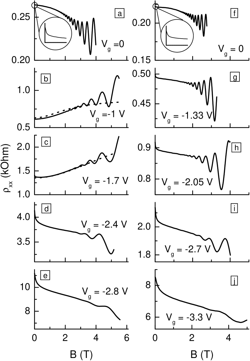
Figure 2: The magnetic field dependences of $\rho_{xx}$ for pattern (left column) and unpattern (right column) structures for $T=4.2$ K. The dotted lines in (b) and (c) are calculated from the standard classical formula for two types of carriers with the electron densities found from Eqs. (1) and (2), and $\mu_{1}=12600$ cm²/(V s), $\mu_{2}=3400$ cm²/(V s) for $V_{g}=-1$ V, and $\mu_{1}=8600$ cm²/(V s), $\mu_{2}=1300$ cm²/(V s) for $V_{g}=-2.4$ V that corresponds to the model described in the text.

The magnetic field dependences of the longitudinal resistance ($\rho_{xx}$) for the pattern structure together with that for the unpattern one for some gate voltages are shown in Fig. 2. It is seen that they are rather complicated. Following the sharp magnetoresistivity in low magnetic field, which results from the suppression of the interference quantum correction, the relatively smooth negative or positive magnetoresistivity against the background of the Shubnikov-de Haas (SdH) oscillations is observed.

Let us first consider the range of high magnetic field. At $V_{g}=0$ the magnetoresistance in the pattern and unpattern structures are very close to each other [see Figs. 2(a) and 2(f)]. In both cases the paraboliclike negative magnetoresistance resulting from the e-e interaction correction (for more detail see Ref. our1, ) and the SdH oscillations of close frequency are observed. Such the behavior is not surprising since the difference in local electron densities in quantum well under the holes and out of them, $\delta n$, is relatively small at $V_{g}=0$. It can be estimated as $\delta n\approx(C_{2}-C_{1})V_{s}/|e|$, where $V_{s}$ is the surface potential, $C_{1,2}=\varepsilon\varepsilon_{0}/t_{1,2}$ is the local capacity, $t_{1,2}$ is the distance between 2D gas and gate electrode in different locations of the structure [see Fig. 1(a)], $\varepsilon_{0}$ is dielectric constant of free space. With the use of $V_{s}\simeq 0.7$ V, $t_{1}=85$ nm, $t_{2}=125$ nm, and $\varepsilon=12.5$ we obtain $\delta n/n\approx 0.1$. However, $\delta n$ strongly increases with the lowering gate voltage that leads to the positive magnetoresistance evident in the pattern sample within the gate voltage range from $-1$ V to $-1.8$ V. The rise of the positive magnetoresistance is a sequence of the comparable contributions to the conductivity from the regions under the holes and out of them. For the first approximation the transport in such inhomogeneous media can be considered as determined by two types of carriers with the different mobility and density.footn1 The dotted curves in Figs. 2(b) and 2(c) are the magnetoresistivity calculated in the framework of this simple model with parameters determined below. At $V_{g}<-1.8$ V, the negative magnetoresistance is restored because the dielectric holes in 2D gas are formed and the conductivity of the structure is determined by the channels between the antidots.

As figure 2 shows the SdH oscillations in the pattern structure are observed down to $V_{g}=-2.8$ V. The periods of the oscillations in the pattern and unpattern structures at given $V_{g}$ are close to each other [see Fig. 3(a)] and the gate voltage dependence of the electron density calculated from the oscillations is well described by the expression

$$n_{1}(V_{g})=n(V_{g})=(1.52+0.33\,V_{g})\times 10^{12},\,\text{cm}^{-2}.$$ (1)

The facts that the oscillations of only one period are observed in the pattern sample and the dependences $n_{1}(V_{g})$ and $n(V_{g})$ are practically the same mean that only the areas of 2D gas located out of the holes contribute to the SdH oscillations. The areas under various holes have probably different electron density due to the different depths of the holes and, therefore, the corresponding oscillations are very broadened. The $V_{g}$ dependence of the electron density under the holes $n_{2}(V_{g})$ can be obtained from the geometric consideration. With the use of the local cap layer thickness $t_{2}=125$ nm we have

$$n_{2}(V_{g})=(1.35+0.55\,V_{g})\times 10^{12},\,\text{cm}^{-2}.$$ (2)

In Fig. 3(a) this dependence is shown by dashed line.

Thus analyzing the high-field magnetoresistance we reason that: (i) at $V_{g}<-1.8$ V the conductivity is mainly determined by the channels; (ii) the electron density out of the dielectric holes remains more or less homogeneous in this $V_{g}$ range.

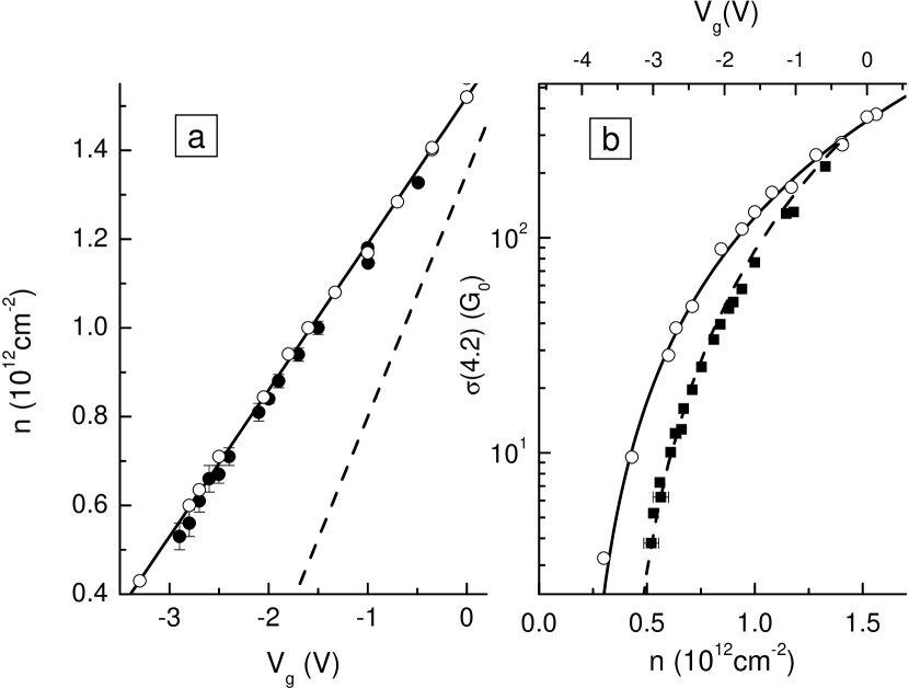
Figure 3: (a) The gate voltage dependence of the electron density found from the SdH oscillations for the pattern (solid symbols) and unpattern (open symbols) structure. Solid and dashed lines are drawn according to Eqs. (1) and (2), respectively. (b) The electron density dependences of the conductivity measured at $T=4.2$ K for the pattern (solid symbols) and unpattern (open symbols).

Let us compare the behavior of the conductivity for pattern ($\sigma_{patt}$) and unpattern ($\sigma_{unpatt}$) samples at $B=0$. The values of $\sigma_{patt}$ and $\sigma_{unpatt}$ measured at $T=4.2$ K are plotted against the electron density found from the SdH oscillations in Fig 3(b). It is seen that the conductivity of the pattern structure significantly steeper falls down with decreasing $n$ than that of unpattern sample. Qualitatively such a behavior is transparent. This is because that the 2D gas under the holes in the pattern sample is depleted faster with lowering $V_{g}$ than that out of them due to thinner cap layer in these locations. If this is the case we can obtain the geometrical parameters of the conducting areas knowing the experimental value of the ratio $\sigma_{unpatt}/\sigma_{patt}$ referred below as $K$. Using the data obtained for the unpattern structure we obtain the mean free path, $l\simeq 0.03\ldots 0.3$ $\mu$m depending on the gate voltage, being less than the characteristic scales of the holes and channels, $\sim 0.5$ $\mu$m [see Fig. 1(b)]. Therefore, one can deal with the local conductivity. If one additionally neglects the randomness in the antidots position, we can write out the following approximate expression for the conductivity of the pattern structure:

$$\sigma_{patt}\simeq\left\{\int_{0}^{D}\frac{dy}{\sigma_{1}w(y)+\sigma_{2}[D-w(y)]}\right\}^{-1}.$$ (3)

where $\sigma_{1}$ and $\sigma_{2}$ stand for the local conductivity of the 2D gas out of and under the holes (in the insert of Fig. 4(a) these areas labeled as 1 and 2, respectively), $w(y)$ is the $y$-dependent width of the area 1. In what follows we suppose the area 2 being round in the shape. The above equation gives the result, which coincides with the exact solution with the accuracy better than $20$ percent when $w_{0}/D>0.1$, where $w_{0}=w(D/2)$. In order to calculate the dependence $K(V_{g})$ it is natural to suppose that the local conductivity $\sigma_{1}$ and $\sigma_{2}$ is fully determined by the local electron density $n_{1}$ and $n_{2}$, respectively, and the $\sigma_{i}$-vs-$n_{i}$ behavior is just the same as that for the unpattern sample $\sigma_{1}(n_{1})$, $\sigma_{2}(n_{2})=\sigma_{unpatt}(n)$ [shown by open symbols in Fig. 3(b)].

In Fig. 4(a) we present the $K$-vs-$n_{1}$ dependences as they have been obtained experimentally and calculated from Eq. (3) with $d=0.7$ $\mu$m obtained from AFM. It is seen that the above simple model well describes the experimental results down to $n_{1}\simeq 8.5\times 10^{11}$ cm^-2 that corresponds to $V_{g}\simeq-2$ V. The reason for the discrepancy which is clearly evident at lower electron density is transparent. For the fixed $d$ value, the saturation of the calculated $K$-vs-$n_{1}$ dependence at $n_{1}<8.5\times 10^{11}$ cm^-2 ($V_{g}\lesssim-2$ V) results from the fact that $\sigma_{2}$ becomes much less than $\sigma_{1}$. The enhance of $K$ obtained experimentally for these gate voltages is sequence of the depletion of the area outside the antidots, i.e., of an increase of the antidots size $d$ and decrease of the channel width $w_{0}=D-d$. Thus knowing the experimental value of $K$ and using Eq. (3) we are able to find the channel width $w_{0}$ when $n_{1}\lesssim 8.5\times 10^{11}$ cm^-2 . The results are depicted in Fig. 4(b). It is seen that the separation between antidots $w_{0}$ decreases with $n_{1}$ decrease. Extrapolating the $w_{0}$-vs-$n_{1}$ plot to $w_{0}=0$ one obtains that the antidots close when $n_{1}\simeq 4\times 10^{11}$ cm^-2 [$V_{g}=-(3.4\ldots 3.2)$ V].

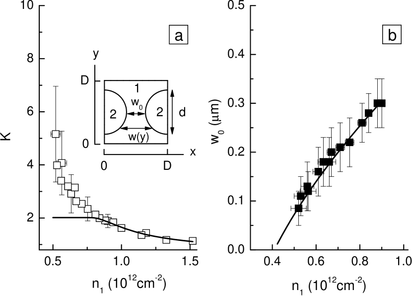
Figure 4: (a) The $K$-vs-$n_{1}$ dependence obtained experimentally (symbols) and calculated from Eq. (3) (lines) for $d=0.7$ $\mu$m and $D=1$ $\mu$m. Insert shows one period of the antidots array. (b) The $n_{1}$ dependence of the channel width $w_{0}$ obtained from the experimental values of $K$ at low $V_{g}$ with the help of Eq. (3). The line is provided as a guide for the eye.

Thus, the gate voltage dependence of the conductivity and the high magnetic field magnetoresistance are reasonably described within the following simple model. At $V_{g}\simeq(0\ldots-2)$ V the conductivity is determined both by the areas under holes and out of the them. These areas are characterized by the different electron density, which determines the local conductivity. At $V_{g}\simeq-(2\ldots 3)$ V the antidots are formed and the conductivity of structure is determined by the channels between the antidots with local conductivity $\sigma_{1}$ equal to the conductivity $\sigma$ of the unpattern sample at the same electron density. Finally, at $V_{g}=-(3.4\ldots 3.2)$ V the channels are collapsed and most likely the crossover to the hopping conductivity should occur.

Let us now inspect the low magnetic field negative magnetoresistivity which results from suppression of the WL correction. We focus our consideration on the results obtained within the second range of the gate voltages: $V_{g}\simeq-(2\ldots 3)$ V. The magnetic field dependences of the local conductivity measured in units of $G_{0}=e^{2}/(2\pi^{2}\hbar)\simeq 1.23\times 10^{-3}$ $\Omega^{-1}$ are presented for different temperatures in Fig. 5(a). For comparison, the analogous dependences for the unpattern structure measured at close conductivity value are shown in Fig. 5(b). For the first sight the magnetoresistance curves in the panels are very similar. However, this impression is wrong. The difference in magnetoresistivity shape for these structures is more pronounced when comparing the results of data treatment performed in a standard manner.

The shape of low-field positive magnetoconductivity $\Delta\sigma(B)=\rho_{xx}^{-1}(B)-\rho_{xx}^{-1}(0)$ caused by suppression of the weak localization in homogeneous 2D gas is described by the Hikami-Larkin-Nagaoka (HLN) expressionhik ; schm

$$\Delta\sigma(B) = \alpha\,G_{0}\,{\cal H}\left(\frac{\tau}{\tau_{\phi}},\frac{B}{B_{tr}}\right),$$

$${\cal H}(x,y) = \psi\left(\frac{1}{2}+\frac{x}{y}\right)-\psi\left(\frac{1}{2}+\frac{1}{y}\right)-\ln{x},$$ (4)

where $B_{tr}=\hbar/(2el^{2})$ is the transport magnetic field, $\tau$ is the momentum relaxation time, $\psi(x)$ is a digamma function, and $\alpha$ is the prefactor, which is equal to unity in the diffusion regime ($B<B_{tr}$, $\tau\ll\tau_{\phi}$) and at high conductivity ($\sigma\gg G_{0}$).

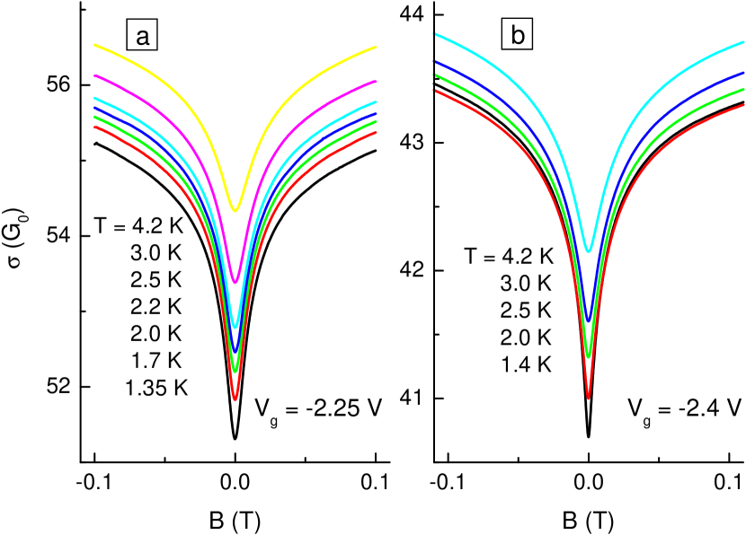
Figure 5: (Color online) The low-field magnetoconductivity for different temperatures for the pattern (a) and unpattern (b) structure. The local conductivity is shown in panel (a).

We have used this expression to fit each experimental curve within different range of magnetic field with $\alpha$ and $\tau_{\phi}$ as the fitting parameters. The results are shown in Fig. 6. How the fitting parameters $\tau_{\phi}$ and $\alpha$ depend on the range of magnetic field is shown in Figs. 6(a) and 6(b), whereas their temperature dependence is shown in Figs. 6(c) and 6(d). One can see that the parameters found for the unpattern structure behave themselves reasonable. Their values only slightly depend on the fitting interval.footn2 The prefactor is close to unity and practically independent of temperature. The temperature dependence of $\tau_{\phi}$ is close to the theoretical one $\tau_{\phi}\propto 1/T$. Thus, the HLN expression well describes $\Delta\sigma(B)$ for the unpattern sample.

In contrast to this, the strong sensitivity of the fitting parameters to the fitting interval takes place for the pattern sample. Therewith the value of $\alpha$ is significantly larger than unity and strongly dependent on the temperature. The value of the fitting parameter $\tau_{\phi}$ is much less than that for the unpattern structure and it saturates with the decreasing temperature. All of this means that the WL correction for the pattern structure is not described by Eq. (4) and the determination of the phase breaking time by the standard way is impossible.footn3

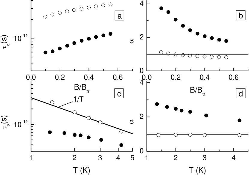
Figure 6: The magnetic field and temperature dependences of the fitting parameters $\tau_{\phi}$ and $\alpha$ for pattern (solid symbols) and unpattern (open symbols) structures. The data in (a) and (b) are shown for the lowest temperatures, the data in (c) and (d) are obtained for the fitting interval from 0 up to $0.25B_{tr}$.

The strong dependence of the fitting parameters on the fitting interval of the magnetic field indicates that the role of dielectric antidots in 2D gas is not reduced to arising of the prefactor $\exp{(-\tau_{E}/\tau_{\phi})}$ with $\tau_{E}$ as the Ehrenfest time, which suppresses the weak localization in the 2D gas with hard discs as scatterersaleiner9697 ; whit08 ; exper4 .

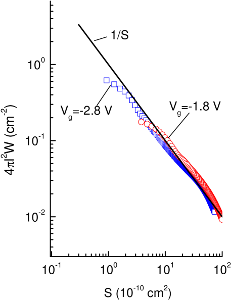
Figure 7: (Color online) The area distribution function $W(S)$ obtained experimentally for the unpattern samples for two gate voltages (symbols). Line is the diffusion limit: $4\pi l^{2}W=1/S$.

Specific features of the weak localization in the pattern sample can be understood by considering the quasiclassic interpretation of this phenomenon. Within quasiclassic approximation the conductivity correction is expressed through the classical quasiprobability for an electron to return to the area of the order $\lambda_{F}l$ ($\lambda_{F}=2\pi/k_{F}$, $k_{F}$ is the Fermi wave vector) around the start pointgork ; chak ; dyak ; dmit

$$\delta\sigma=-\sigma_{0}\frac{\lambda_{F}l}{\pi}{\cal W},$$ (5)

where $\sigma_{0}=\pi k_{F}lG_{0}$ is the Drude conductivity, and ${\cal W}$ stands for the quasiprobability density of return (quasi- means that ${\cal W}$ includes not only the classical probability density, but the interference destruction due to an external magnetic field and inelastic scattering processes). With taking these effects into account Eq. (5) can be rewritten as followsour2

$$\delta\sigma(b) = -2\pi l^{2}G_{0}\int_{-\infty}^{\infty}dS\ \biggl{\{}W(S)$$ (6)

$$\exp\left[-\frac{\overline{L}(S)}{l_{\phi}}\right]\cos\left(\frac{bS}{l^{2}}\right)\biggr{\}},$$

where $l_{\phi}$ is the phase breaking length connected with $\tau_{\phi}$ through the Fermi velocity, $l_{\phi}=v_{F}\tau_{\phi}$, $W(S)$ and $\overline{L}(S)$ are the algebraic area distribution function of closed paths and the area dependence of the average length of closed paths respectively (for more detail see Sec. II of Ref. our2, ). This equation shows that the shape of the magnetoconductivity curve is determined by the statistics of the closed paths, namely by the area distribution function $W(S)$ and by function $\overline{L}(S)$. It is clear that the existence of dielectric dots in 2D gas should change the statistics of closed paths resulting in the change of the shape of the magnetoconductivity curve. In Ref. our3, , there is shown how the analysis of the Fourier transform of the negative magnetoresistance provides the information on the function $W(S)$. The short of the matter is clear from Eq. (6). It is seen that the Fourier transform of $\delta\sigma(B)$

$$\Phi(S)=\frac{1}{\Phi_{0}}\int_{-\infty}^{\infty}dB\ \delta\sigma(B)\cos\left(\frac{2\pi BS}{\Phi_{0}}\right)$$

is equal to

$$\Phi(S)=-2\pi l^{2}G_{0}W(S)\exp\left(-\frac{\overline{L}(S)}{l_{\phi}}\right),$$ (7)

where $\Phi_{0}=\pi\hbar/e$ is the elementary flux quantum. Since $l_{\phi}$ tends to infinity when $T\to 0$, the extrapolation of $\Phi(S,T)$ to $T=0$ should give the value of $2\pi l^{2}G_{0}W(S)$. It is ideal situation. In the reality, such the approach allows us to obtain experimentally the area distribution function of the trajectories which length is less than approximately $2\,l^{\prime}_{\phi}$, where $l^{\prime}_{\phi}$ is the phase relaxation length at lowest temperature of the experiment, because the contribution of longer trajectories to the magnetoconductivity is very small.

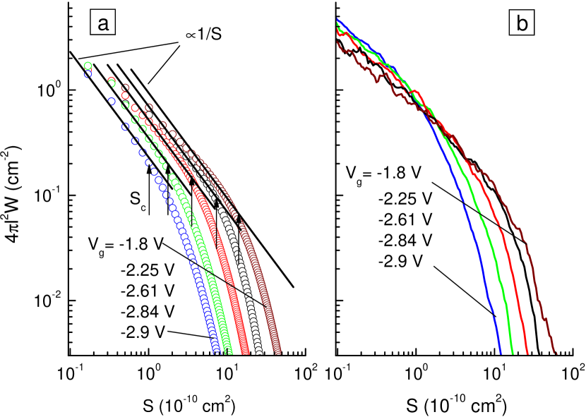
Figure 8: (Color online) (a) The function $4\pi l^{2}W(S)$ obtained experimentally for the pattern sample for different gate voltages. Arrows indicates where the plots deviate from $1/S$-dependence. (b) The function $4\pi l^{2}W(S)$ obtained from the simulation procedure carried out with parameters corresponding to the gate voltages in panel (a).

The results of the data processing for the unpattern and pattern samples are shown in Figs. 7 and 8(a), respectively (note the scales in these figures are identical). It is seen that not only the $W$-vs-$S$ dependences are drastically different for the pattern and unpattern samples but their responses to the change of the gate voltage as well. The area distribution function for the unpattern sample is very close to that predicted theoretically for 2D homogeneous systems in the diffusion regime, $4\pi l^{2}W=S^{-1}$, $S>l^{2}$ (see Refs. our2, and our3, ), it is practically insensitive to the gate voltage (Fig. 7). As for the pattern sample, it is seen that the curves follow near the $1/S$ dependence only at low $S<S_{c}$ values. At higher areas, $S>S_{c}$, $W$ decreases with $S$ increase much steeper than $S^{-1}$; the lower gate voltage is the lower areas $S_{c}$ at which this deviation occurs [Fig. 8(a)].

Before to interpret such the behavior of $W(S)$ for the pattern sample let us clarify the meaning of this quantity for this case. Because our system is inhomogeneous due to dielectric inclusions under the holes in the cap layer, Eq. (6) should be rederived. This is because the function $W(S)$ is not universal now, it should depend on the position of starting point. If one neglects as above the aperiodicity of the antidots array, we obtains the following expression connecting the correction to the conductivity of the antidots array and local correction $\delta\sigma_{l}$:

$$\delta\sigma(b)=\frac{\displaystyle\int\frac{dy}{[w(y)]^{2}}\int dx\,\delta\sigma_{l}(x,y,b)}{\left[\displaystyle\int\frac{dy}{\displaystyle w(y)}\right]^{2}}.$$ (8)

Here, the integration runs over the intervals given by the border of conducting area, $w(y)$ is the $y$ dependence of width of conducting area, and the quantity $\sigma_{l}(x,y,b)$ is given by the expression analogous to Eq. (6):

$$\delta\sigma_{l}(x,y,b) = -2\pi l^{2}G_{0}\int_{-\infty}^{\infty}dS\ \biggl{\{}\mathfrak{W}(x,y,S)$$ (9)

$$\exp\left[-\frac{\overline{L}(x,y,S)}{l_{\phi}}\right]\cos\left(\frac{bS}{l^{2}}\right)\biggr{\}},$$

in which $\mathfrak{W}(x,y,S)$ is determined in such a way that $\mathfrak{W}(x,y,S)dS$ gives the density probability of return to the starting point with the coordinates $(x,y)$ with the enclosed algebraic area in the interval $(S,S+dS)$.

Thus, the above described procedure, which for the homogeneous 2D gas allows us to obtain the area distribution function of closed paths, being applied to the data obtained for the pattern sample gives the effective area distribution function:

$$W(S)=\frac{\displaystyle\int\frac{dy}{[w(y)]^{2}}\int\mathfrak{W}(x,y,S)\,dx}{\left[\displaystyle\int\frac{dy}{\displaystyle w(y)}\right]^{2}}.$$ (10)

Now we are in position to discuss the behavior of $W(S)$ for the pattern sample [Fig. 8(a)]. In order to understand main features we have performed the computer simulation of a particle motion over 2D plane with scatterers. The details can be found in Refs. our2, ; our4, ; our5, , below is outline only and important features. The 2D plane is represented as a lattice with scatterers of two types placed in a part of lattice site. The scatterers of the first type with isotropic differential cross-section correspond to ionized impurity. The scatterers of the second type are hard discs with specular reflection from the boundaries. Particle motion is forbidden within the disks. They correspond to the areas of 2D gas under the holes. A particle is launched from some point with $x,y$ as coordinates, then it moves with a constant velocity along straight lines, which happen to be terminated by collisions with the scatterers. After collision it changes the motion direction. If the particle passes near the starting point at the distance less than some prescribed value $a/2\ll l$, the path is perceived as being closed. Its length and enclosed algebraic area are calculated and kept in memory. The particle walks over the plane until the path traversed is longer than $2l^{\prime}_{\phi}$, where $l^{\prime}_{\phi}$ is the phase relaxation time obtained at lowest temperature on the unpattern sample for the same $V_{g}$ value. As mentioned above namely the statistics of such closed paths can be reliably obtained from the weak localization experiments. When the path becomes longer than this value another particle is launched and all is repeated. After large number of launches from the starting point with given $x,y$ coordinates $\mathfrak{W}(x,y,S)$ is calculated as

$$\mathfrak{W}(x,y,S)=\frac{n_{S}}{N\,l\,a\,\Delta S},$$ (11)

where $N$ is the number of starts from this point, $n_{S}$ is the number of returns along the trajectory with enclosed area in the interval $(S,S+\Delta S)$. Launching the particle from different starting points, we are able to calculate numerically the function $W(S)$ using Eq. (10) in the discrete form.

Shown in Fig. 8(b) are the results of simulation procedure carried out with the parameters corresponding to the gate voltages from Fig. 8(a). It is clearly seen that the results of computer simulation are in qualitative agreement with those of real experiment.

Analysis of the simulation results gives an insight into why the experimental $W$-vs-$S$ dependence is steeper for the pattern sample. This can be done if one considers how the paths with the given area enclosed are distributed over the length. This distribution is characterized by the function $w_{S}(L)$ determined in such a way that $w_{S}(L)dS$ gives the density probability of return along a trajectory with the length $L$ and area in the interval $(S,S+dS)$. In Fig. 9 we show the functions $w_{S}(L)$ obtained from the simulation procedure for the patternfootn4 and unpattern samples (all the paths including those for which $L>2\,l^{\prime}_{\phi}$ are taken into account here). Qualitatively, the functions are similar. They have a peak which position characterizes the typical length of closed paths. In both cases, the larger area enclosed the longer trajectories. The $w_{S}$-vs-$L$ plot for the unpattern sample is well described by the expression

$$w_{S}(L)=\frac{1}{(2\,l\,L)^{2}}\cosh^{-2}\left(\frac{\pi S}{l\,L}\right)$$ (12)

obtained analytically within the diffusion approximation for the ordinary 2D systemour2 that justifies the validity of simulation procedure. An important point is that the closed paths in the pattern sample are significantly longer than the paths in the unpattern sample with the same area enclosed. If, in correspondence with the experimental situation, one restricts the consideration by short trajectories, $L\lesssim 2\,l^{\prime}_{\phi}$, we obtain

$$W(S)=\int_{0}^{2\,l^{\prime}_{\phi}}w_{S}(L)\frac{dL}{l}.$$ (13)

approximately the same for the both samples when $S$ is relatively small [Figs. 9(a)], and much less in the pattern sample when $S$ is sufficiently large [Fig. 9(c)]. Thus, the different length distribution of closed paths is the reason of the different behavior of the area distribution function obtained experimentally for the pattern and unpattern samples.

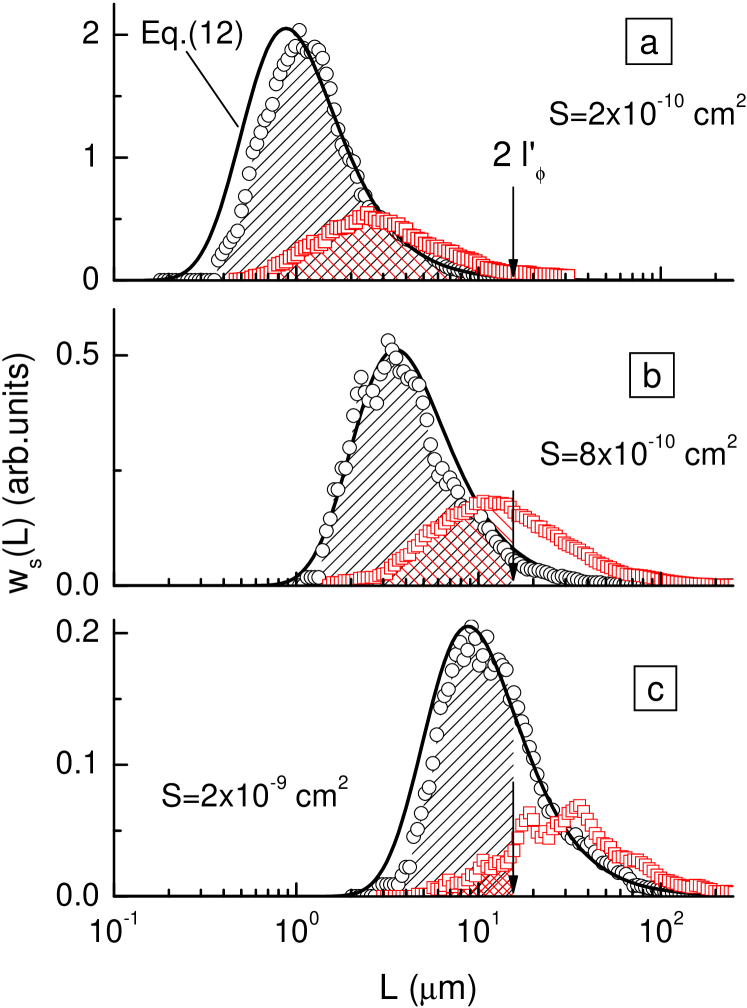
Figure 9: (Color online) The length distribution functions of closed paths with different area enclosed obtained from the simulation procedure with parameters corresponding to the unpattern (circles) and pattern (squares) samples for $V_{g}=-2.84$ V. Lines are calculated from Eq. (12) with corresponding $S$-values and $l=0.06$ $\mu$m. Hatched areas are the $W$ value for paths with $L\leq 2\,l^{\prime}_{\phi}$.

Let us return to the magnetoconductivity caused by suppression of the interference quantum correction. The simulation procedure allows us to calculate $\delta\sigma(b)$ for the model system. This can be done with the use of Eq. (8) in the discrete form and of $\delta\sigma_{l}(x,y,b)$ calculated as

$$\delta\sigma_{l}(x_{i},y_{i},b)=\frac{2\pi lG_{0}}{d\,N_{i}}\sum_{k}\cos\left(\frac{bS_{i}^{k}}{l^{2}}\right)\exp{\left(-\frac{l_{i}^{k}}{l_{\phi}}\right)},$$ (14)

where summation runs over all closed trajectories among a total number of trajectories $N_{i}$ starting from the point with $x_{i}$ and $y_{i}$ as coordinates, $S_{i}^{k}$ and $l_{i}^{k}$ stand for algebraic area and length respectively of the $k$-th trajectory.

In Fig. 10 we compare the simulation and experimental results. Symbols are the experimental plot obtained for the pattern sample at $V_{g}=-2.25$ V. Solid lines are the simulated magnetic field dependences of $\Delta\sigma=\delta\sigma(B)-\delta\sigma(0)$. The values of $\tau_{\phi}=1.9\times 10^{-11}$ s for $T=1.35$ K and $\tau_{\phi}=6.8\times 10^{-12}$ s for $T=4.2$ K correspond to the best accordance with the experimental data. It is significant that they are close to that obtained for the unpattern sample [see Fig. 6(c)]. If one calculates $\Delta\sigma(B)$ from Eq. (4) with the same parameters and $\alpha=1$ we obtain drastic disagreement with the experimental magnetoconductance (see dashed lines Fig. 10).

Thus, the simulation approach allows us to understand qualitatively the main features of the low-field magnetoconductivity in the pattern samples, which are determined by peculiarities of statistics of closed paths.

It would serve no purpose to make more detailed comparison between the experimental and simulation results because our model is rather crude. So, we supposed that the areas forbidden for classical motion had the form of hard disks. As seen from Fig. 1(b) it is not exactly. Moreover, it was suggested that the mean free path and Fermi velocity are constant over all the conducting area that should not be fulfilled in the real structures.

In summary, we have studied the weak localization in the 2D electron gas with potential electrostatic relief forming the insulating antidots array. It has been shown that the use of the standard procedure for the obtaining of the phase relaxation time from the shape of the magnetoconductivity curve is inadequate when it is applied to the antidots array structure in the diffusion regime. To understand the main features of the weak localization in these systems the alternative approach based on the analysis of the statistics of closed paths has been used. We have shown that the main peculiarities of the WL phenomenon in the pattern structure are due to the specific statistics of closed paths. The paths of actual areas in system with antidots are characterized by significantly larger lengths as compared with the usual 2D systems.

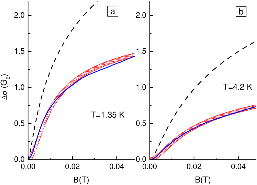
Figure 10: (Color online) The low-field magnetoconductance for the pattern sample for $T=1.35$ K (a) and $4.2$ K(b), $V_{g}=-2.25$ V. Symbols are the measured dependences. Solid and dashed lines are the simulation results and Eq. (4) obtained with $\tau_{\phi}=1.9\times 10^{-11}$ s (a) and $\tau_{\phi}=6.8\times 10^{-12}$ s (b).

References

- (1) K. Enslin and P. M. Petrov, Phys. Rev. B 41, 12307 (1990).
- (2) D. Weiss, M. L. Roukes, A. Menschig, P. Grambow, K. von Klitzing, and G. Weimann, Phys. Rev. Lett. 66, 2790 (1991).
- (3) A. M. Chang, H. U. Baranger, L. N. Preffer, and K. W. West, Phys. Rev. Lett. 73, 2111 (1994).
- (4) M. V.Budantsev, Z. D.Kvon, A. G.Pogosov, G. M. Gusev, J. C. Portal, D. K. Maude, N. T. Moshegov, and A. I. Toropov, Phisica B, 256-258, 595 (1998).
- (5) Oleg Yevtushenko, Gerd Lutjering, Dieter Weiss, and Klaus Richter, Phys. Rev. Lett. 84, 542 (2000).
- (6) J. A. Folk, C. M. Marcus and J. S. Harris, Phys. Rev. Lett. 87, 206802 (2001).
- (7) A. Pouydebasque, A. G. Pogosov, M. V. Budantsev, A. E. Plotnikov, A. I. Toropov, D. K. Maude, and J. C. Portal, Phys. Rev. B 64, 245306 (2001).
- (8) Z. D. Kvon, Pis’ma Zh. Eksp. Teor. Fiz. 76, 619 (2002) [JETP Lett. 76, 537 (2002)].
- (9) August Dorn, Thomas Ihn, Klaus Ensslin, Werner Wegscheider, and Max Bichler, Phys. Rev. B 70, 205306 (2004).
- (10) M. Ferrier, L. Angers, A. C. H. Rowe, S. Gueron, H. Bouchiat, C. Texier, G. Montambaux, and D. Mailly, Phys. Rev. Lett. 93, 246804 (2004).
- (11) B. Hackens, S. Faniel, C. Gustin, X. Wallart, S. Bollaert, A. Cappy, and V. Bayot, Phys. Rev. Lett. 94, 146802 (2005).
- (12) I. L. Aleiner, A. I. Larkin, Phys. Rev. B 54, 14423 (1996).
- (13) D. G. Polyakov, F. Evers, A. D. Mirlin, and P. Wölfle, Phys. Rev. B 64, 205306 (2001).
- (14) P. W. Brouwer, J. N. H. J. Cremers, and B. I. Halperin, Phys. Rev. B 65, 081302 (2002).
- (15) D.S. Golubev and A.D. Zaikin, Phys. Rev. B 74, 245329 (2006).
- (16) Iva Bezinová, Christoph Stampfer, Ludger Wirtz, Stefan Rotter, Joachim Burgdörfer, Phys. Rev. B 77, 165321 (2008).
- (17) G. M. Minkov, A. V. Germanenko, O. E. Rut, A. A. Sherstobitov, V. A. Larionova, A. K. Bakarov, and B. N. Zvonkov, Phys. Rev. B 74, 045314 (2006).
- (18) Another way of description of the positive magnetoresistance is considering of interplay between short and long range disorder in the magnetic field.Theory1
- (19) S. Hikami, A. Larkin and Y. Nagaoka, Prog. Theor. Phys. 63, 707 (1980).
- (20) H.-P. Wittman and A. Schmid, J. Low. Temp. Phys. 69, 131 (1987).
- (21) Some rise of with extending fitting interval evident in Fig. 6(a) is a sequence of the fact that the magnetic field dependence of is not take into account in Eq. (4) [see for details A. V. Germanenko, V. A. Larionova, I. V. Gornyi, and G. M. Minkov, Int. J. Nanosci. 6, 261 (2007)].
- (22) I. L. Aleiner and A. I. Larkin, Phys. Rev. B 54, 14423 (1996); Chaos Solitons Fractals 8, 1179 (1997).
- (23) Robert S. Whitney, Philippe Jacquod, and Cyril Petitjean, Phys. Rev. B 77, 045315 (2008).
- (24) In this connection the low- saturation of reported in some paper for granular metal films [see, e.g., X.X. Zhang, Chuncheng Wan, H. Liu, Z.Q. Li, and Ping Sheng, Phys. Rev. Lett. 86, 5562 (2001)] is questionable.
- (25) L. P. Gorkov, A. I. Larkin, and D. E. Khmelnitskii, Pis’ma Zh. Eksp. Teor. Fiz. 30, 248 (1979) [JETP Lett. 30, 228 (1979)].
- (26) S. Chakravarty and A. Schmid, Phys. Reports 140, 193 (1986).
- (27) M. I. Dyakonov, Solid St. Comm. 92, 711 (1994).
- (28) I. V. Gornyi, A. P. Dmitriev, and V. Yu. Kachorovskii, Phys. Rev. B 56, 9910 (1997).
- (29) G. M. Minkov, A. V. Germanenko, V. A. Larionova, and S. A. Negashev, and I. V. Gornyi, Phys. Rev. B 61, 13164 (2000).
- (30) G. M. Minkov, S. A. Negashev, O. E. Rut, A. V. Germanenko, O. I. Khrykin, V. I. Shashkin, and V. M. Danil tsev, Phys. Rev. B 61, 13172 (2000).
- (31) A. V. Germanenko, G. M. Minkov, and O. E.Rut, Phys.Rev.B 64, 165404 (2001).
- (32) A. V. Germanenko, G. M. Minkov, A. A. Sherstobitov, and O. E. Rut Phys. Rev. B 73, 233301 (2006).
- (33) For the pattern sample, the effective length distribution function defined by analogy with Eq. (10) is presented.