The Ginibre ensemble of real random matrices and its scaling limits

Abstract

We give a closed form for the correlation functions of ensembles of a class of asymmetric real matrices in terms of the Pfaffian of an antisymmetric matrix formed from a $2\times 2$ matrix kernel associated to the ensemble. We apply this result to the real Ginibre ensemble and compute the bulk and edge scaling limits of its correlation functions as the size of the matrices becomes large.

1 Introduction

The principal subject of this paper is the Ginibre ensemble of real random matrices — square real valued matrices with i.i.d. normal entries. Random matrix models have been very successful in describing various physical phenomena. (See e.g. [16] and references therein). Physical applications of the Ginibre ensembles are described in [13], [17] and [12]. Mathematically, the ability to analyze spectra of random matrices is largely based on determinental or Pfaffian formulas for spectral correlations that have been derived for a variety of models. The real Ginibre ensemble is one of the few models for which such formulas remained unavailable for over 40 years (the model was introduced by Ginibre in 1965 [14]). The goal of this paper is to prove Pfaffian formulas for all the correlation functions of the real Ginibre ensemble and to evaluate their bulk and edge scaling limits.

The algebraic techniques that we use were developed in a recent work of the second author [21]. Starting from that paper, Forrester and Nagao [12] have independently obtained similar Pfaffian formulas for correlations and constructed certain skew-orthogonal polynomials necessary for the asymptotic analysis. We take the next step and obtain the asymptotics of the correlation functions using these polynomials.

In the algebraic part of this paper we consider a general class of probability measures that includes the real Ginibre ensembles and ensembles arising in the study of Mahler measure of polynomials; the latter are of interest in number theory, see [22]. We show that the correlation functions for an ensemble from this class can be expressed as the Pfaffian of a block matrix whose entries are expressed in terms of a $2\times 2$ matrix kernel associated to the ensemble. We find much inspiration from Tracy and Widom’s paper on correlation and cluster functions of Hermitian and related ensembles [26]. However, instead of using properties of the Fredholm determinant to calculate the correlation functions via the cluster functions, we use the notion of the Fredholm Pfaffian to determine the correlation functions directly. A Pfaffian analog of the Cauchy-Binet formula introduced by Rains [20] lies at the heart of our proof. For completeness we will include Rains’ proof here. In place of the identities of de Bruijn [7] used by Tracy and Widom we will use an identity of the second author [21] to compute the correlation functions for ensembles of asymmetric matrices. Rains’ Cauchy-Binet formula has applicability in a wider context than just the determination of the correlation function for ensembles of asymmetric matrices, and we will use it to give a simplified proof of the correlation function of Hermitian ensembles of random matrices when $\beta=1$ and $\beta=4$.

We then apply our theory to the real Ginibre ensemble. It is known (see [15] [2] [9] [8]) that the density functions of real and complex eigenvalues is approximately constant on $(-\sqrt{N},\sqrt{N})$ and the disc of radius $\sqrt{N}$ respectively (here $N$ is the size of the matrices). We study the local correlations of eigenvalues in four different regions: near a real point $u\sqrt{N}$ with $-1<u<1$ (real bulk), near $\pm\sqrt{N}$ (real edge), near a (non-real) complex point $u\sqrt{N}$ with $|u|<\sqrt{N}$ (complex bulk), and near $u\sqrt{N}$ with $|u|=\sqrt{N},$ $\mathrm{Im}(u)\neq 0$ (complex edge). Four different limit processes arise, and we compute their correlation functions explicitly. The complex bulk and edge limits turn out to be the same as in the case of the much simpler complex Ginibre ensembles. The correlations of real eigenvalues in the real bulk region were obtained in [12] and the density functions were computed earlier using different techniques [8] [9]. All other results appear to be new.

The paper is organized as follows. Section 2 introduces necessary notation. In Section 3, we introduce a class of ensembles relevant for our study. In Section 4 we show that the real Ginibre ensemble and the ensemble related to Mahler measure fall into this class. In Section 5, we introduce the correlation functions. In Section 6 we construct the correlation kernel, and in Section 7 we state how the correlation functions are expressed through that kernel. Section 8 contains statements of asymptotic results as well as the limiting correlation kernels. Section 9 contains the proofs. Appendix A shows how to apply Rains’ Cauchy-Binet formula to the $\beta=1,4$ Hermitian random matrix ensembles. Appendix B contains the proof of Rains’ formula. In Appendix C we compute the bulk and edge limits of the complex Ginibre ensemble. (We were unable to locate this material in the literature). Appendix D provides plots of the first and second correlation functions in various limit regimes.

Acknowledgments. We thank Percy Deift for helpful early discussions and for introducing the authors to each other. The second author would also like to thank Brian Rider for many helpful discussions regarding the Ginibre real ensemble. We are grateful to Eric Rains for allowing us to include his proof of the the Pfaffian Cauchy-Binet formula (Appendix B). Finally we would like to thank Peter Forrester for keeping us updated about his work. The first named author (A.B.) was partially supported by the NSF grant DMS-0707163.

2 Point Processes on the Space of Eigenvalues of $\mathbb{R}^{N\times N}$

We start rather generally since the results in this manuscript can be used to describe not only the statistics of eigenvalues of ensembles of real matrices but also the statistics of roots of certain ensembles of real polynomials. We begin with random point processes on two-component systems.

Let $X$ be the set of finite multisets of the closed upper half plane $\overline{H}\subset\mathbb{C}$. An element $\xi\in X$ is called a configuration, and $X$ is called the configuration space of $\overline{H}$. Given a Borel set $A$ of $\overline{H}$, we define the function $\mathcal{N}_{A}:X\rightarrow\mathbb{Z}^{\geq 0}$ by specifying that $\mathcal{N}_{A}(\xi)$ be the cardinality (as a multiset) of $(\xi\cap A)$. We define $\Sigma$ to be the sigma-algebra on $X$ generated by $\{\mathcal{N}_{A}:A\subseteq\overline{H}\mbox{ Borel}\}$. A probability measure $\mathcal{P}$ defined on $\Sigma$ is called a random point process on $X$.

For each pair of non-negative integers $(L,M)$ we define $X_{L,M}$ to be the subset of $X$ consisting of those configurations $\xi$ which consist of exactly $L$ real points and $M$ points in the open upper half plane $H$. That is,

$$X_{L,M}:=\big{\{}\xi\in X:\mathcal{N}_{\mathbb{R}}(\xi)=L\mbox{ and }\mathcal{N}_{H}(\xi)=M\big{\}}.$$

Clearly, $X_{L,M}$ is measurable and $X$ can be written as the disjoint union

$$X=\bigcup_{L\geq 0,M\geq 0}X_{L,M}.$$

Given a point process $\mathcal{P}$ on $X$, we may define the measure $\mathcal{P}_{L,M}$ on $X$ by $\mathcal{P}_{L,M}(B):=\mathcal{P}(B\cap X_{L,M})$ for each $B\in\Sigma$ . The measure $\mathcal{P}_{L,M}$ induces a measure on $X_{L,M}$ (and we will also use the symbol $\mathcal{P}_{L,M}$ for this measure).

Given a matrix $\mathbf{Y}\in\mathbb{R}^{N\times N}$ there must be a pair of non-negative integers $(L,M)$ with $L+2M=N$ such that, counting multiplicities, $\mathbf{Y}$ has $L$ real eigenvalues and $M$ non-real complex conjugate pairs of eigenvalues. By representing each pair of complex conjugate eigenvalues by its representative in $H$, we may identify all possible multisets of eigenvalues of matrices in $\mathbb{R}^{N\times N}$ with the disjoint union

$$X_{N}:=\bigcup_{(L,M)\atop L+2M=N}X_{L,M}.$$ (2.1)

Similarly, we may identify all possible multisets of roots of degree $N$ real polynomials with this disjoint union. Thus, when studying the statistics of eigenvalues of ensembles of asymmetric real matrices (respectively of the roots of degree $N$ real polynomials) we may restrict ourselves to random point processes on $H$ which are supported on the disjoint union given in (2.1). That is, the eigenvalue statistics of an ensemble of real matrices is determined by a set of finite measures $\mathcal{P}_{L,M}$ on $X_{L,M}$ for each pair of non-negative integers $(L,M)$ with $L+2M=N$. In this situation we will say that $\mathcal{P}$ is a random point process on $X_{N}$ associated to the family of finite measures $\{\mathcal{P}_{L,M}:L+2M=N\}$.

From here forward we will assume that $L,M$ and $N$ are non-negative integers such that $L+2M=N$, and a sum indexed over $(L,M)$ will be taken to be a sum over all pairs satisfying this condition. Moreover, when we refer to a point process we will always mean a point process on $X_{N}$.

3 Point Processes on $X_{N}$ Associated to Weights

In this section we will introduce an important class of point processes associated to Borel measures on $\mathbb{C}$. We will be particularly interested in measures which are a sum of two mutually singular measures: one of which is absolutely continuous with respect to Lebesgue measure on $\mathbb{R}$ and one which is absolutely continuous with respect to Lebesgue measure on $\mathbb{C}$. The corresponding densities with respect to Lebesgue measure will allow us to construct a weight function which uniquely determines the associated point process on $X_{N}$. Point processes of this sort arise in the study of asymmetric random matrices and the range of multiplicative functions on polynomials with real coefficients.

It will be useful to distinguish non-real complex numbers and we set $\mathbb{C}_{\ast}=\mathbb{C}\setminus\mathbb{R}$.

We start rather generally by constructing measures on $X_{L,M}$ from measures on $\mathbb{R}^{L}\times\mathbb{C}_{\ast}^{M}$. The benefit in doing this is that it allows us to express important quantities associated to point processes (averages, correlation functions, etc.) as rather pedestrian integrals over $\mathbb{R}^{L}\times\mathbb{C}_{\ast}^{M}$. To each $(\boldsymbol{\alpha},\boldsymbol{\beta})\in\mathbb{R}^{L}\times\mathbb{C}_{\ast}^{M}$ we associate a configuration in $X_{L,M}$ given by

$$\{\boldsymbol{\alpha},\boldsymbol{\beta}\}:=\{\alpha_{1},\ldots,\alpha_{L},\widehat{\beta}_{1},\ldots,\widehat{\beta}_{M}\},\quad\mbox{where}\quad\widehat{\beta_{m}}=\{\beta_{m},\overline{\beta_{m}}\}\cap H.$$

A given configuration $\xi\in X_{L,M}$ may correspond to several vectors in $\mathbb{R}^{L}\times\mathbb{C}_{\ast}^{M}$ and we will call $\{(\boldsymbol{\alpha},\boldsymbol{\beta}):\{\boldsymbol{\alpha},\boldsymbol{\beta}\}=\xi\}$ the set of configuration vectors of $\xi$.

A function $F$ on $X_{L,M}$ induces a function on $\mathbb{R}^{L}\times\mathbb{C}_{\ast}^{M}$ specified by $(\boldsymbol{\alpha},\boldsymbol{\beta})\mapsto F\{\boldsymbol{\alpha},\boldsymbol{\beta}\}$, and given a measure $\nu_{L,M}$ on $\mathbb{R}^{L}\times\mathbb{C}_{\ast}^{M}$ there exists a unique measure $\mathcal{P}_{L,M}$ on $X_{L,M}$ specified by demanding that

$$\int_{X_{L,M}}F(\xi)\,d\mathcal{P}_{L,M}(\xi)=\frac{1}{L!M!2^{M}}\int_{\mathbb{R}^{L}\times\mathbb{C}_{\ast}^{M}}F\{\boldsymbol{\alpha},\boldsymbol{\beta}\}\,d\nu_{L,M}(\boldsymbol{\alpha},\boldsymbol{\beta}),$$ (3.1)

for every $\Sigma$-measurable function $F$ on $X$. The normalization constant $L!M!2^{M}$ arises since a generic element $\xi\in X_{L,M}$ corresponds to $L!M!2^{M}$ configuration vectors. By specifying measures $\nu_{L,M}$ on $\mathbb{R}^{L}\times\mathbb{C}_{\ast}^{M}$ for all pairs $(L,M)$ and normalizing so that the total measure of $X_{N}$ is 1, we define a point process on $X_{N}$.

A very important class of point processes arises when we demand that the various $\nu_{L,M}$ are all related to a single measure on $\mathbb{C}$. Given a measure $\nu_{1}$ on $\mathbb{R}$ and a measure $\nu_{2}$ on $\mathbb{C}_{\ast}$, we set $\nu$ to be the measure $\nu_{1}+\nu_{2}$ on $\mathbb{C}$. We will write $\nu_{L}$ for the product measure of $\nu_{1}$ on $\mathbb{R}^{L}$ and $\nu_{2M}$ will be the product measure of $\nu_{2}$ on $\mathbb{C}^{M}$. By combining $\nu_{L}$ and $\nu_{2M}$ with a certain Vandermonde determinant we will arrive at the desired measures on $\mathbb{R}^{L}\times\mathbb{C}_{\ast}^{M}$. Given a vector $\boldsymbol{\gamma}\in\mathbb{C}^{N}$ we define $V(\boldsymbol{\gamma})$ to be the $N\times N$ matrix whose $n,n^{\prime}$ entry is given by $\gamma_{n}^{n^{\prime}-1}$. We will denote the determinant of $V(\boldsymbol{\gamma})$ by $\Delta(\boldsymbol{\gamma})$, and define the function $\Delta:\mathbb{R}^{L}\times\mathbb{C}^{M}\rightarrow\mathbb{C}$ by

$$\Delta(\boldsymbol{\alpha},\boldsymbol{\beta}):=\Delta(\alpha_{1},\ldots,\alpha_{L},\beta_{1},\overline{\beta_{1}},\ldots,\beta_{M},\overline{\beta_{M}}).$$

Using these definitions we set $\nu_{L,M}$ to be the measure on $\mathbb{R}^{L}\times\mathbb{C}_{\ast}^{M}$ given by

$$\frac{d\nu_{L,M}}{d(\nu_{L}\times\nu_{2M})}(\boldsymbol{\alpha},\boldsymbol{\beta})=2^{M}|\Delta(\boldsymbol{\alpha},\boldsymbol{\beta})|,$$ (3.2)

and we will write $\mathcal{P}_{L,M}^{\nu}$ for the measure on $X_{L,M}$ given specified by $\nu_{L,M}$ as in (3.1). If $\mathcal{P}^{\nu}_{L,M}$ is finite for each pair $(L,M)$, then we set

$$\mathcal{P}^{\nu}:=\frac{1}{Z^{\nu}}\sum_{(L,M)}\mathcal{P}^{\nu}_{L,M}\qquad\mbox{where}\qquad Z^{\nu}:=\sum_{(L,M)}\mathcal{P}_{L,M}^{\nu}(X_{L,M}).$$

We will call $\mathcal{P}^{\nu}$ the point process on $X_{N}$ associated to the weight measure $\nu$ and $Z^{\nu}$ will be referred to as the partition function of $\mathcal{P}^{\nu}$.

We set $\lambda_{1}$ and $\lambda_{2}$ to be Lebesgue measure on $\mathbb{R}$ and $\mathbb{C}$ respectively and let $\lambda:=\lambda_{1}+\lambda_{2}$. If there exists a function $w:\mathbb{C}\rightarrow[0,\infty)$ such that $\nu=w\lambda$ (by which we mean $d\nu/d\lambda=w$), then we will call $w$ the weight function of $\mathcal{P}^{\nu}$. In this situation we set $\mathcal{P}_{L,M}^{w}:=\mathcal{P}_{L,M}^{\nu}$ and define $\mathcal{P}^{w}$ and $Z^{w}$ analogously. If $P^{\nu}$ has weight function $w$ then

$$\frac{d\nu_{L,M}}{d(\lambda_{L}\times\lambda_{2M})}(\boldsymbol{\alpha},\boldsymbol{\beta})=2^{M}\bigg{\{}\prod_{\ell=1}^{L}w(\alpha_{\ell})\prod_{m=1}^{M}w(\beta_{m})\bigg{\}}\big{|}\Delta(\boldsymbol{\alpha},\boldsymbol{\beta})\big{|},$$ (3.3)

and we define $\Omega_{L,M}:\mathbb{R}^{L}\times\mathbb{C}^{M}$ to be the function given on the right hand side of (3.3). The collection $\{\Omega_{L,M}:L+2M=N\}$ plays the role of the joint eigenvalue probability density function, and we will call $\Omega_{L,M}$ the $L,M$-partial joint eigenvalue probability density function of $\mathcal{P}^{w}$.

4 Examples of Point Processes Associated to Weights

Point processes on $X_{N}$ associated to weights arise in a variety of contexts. It is often the case that the weight function $w$ is invariant under complex conjugation. In this situation, there necessarily exists some function $\rho:\mathbb{C}\rightarrow[0,\infty)$ such that

$$w(\gamma):=\left\{\begin{array}[]{ll}\rho(\gamma)&\quad\mbox{if }\gamma\in\mathbb{R};\\ &\\ \rho(\gamma)\rho(\overline{\gamma})&\quad\mbox{if }\gamma\in\mathbb{C}_{\ast}.\end{array}\right.$$

When it exists, we will cal $\rho$ the root or eigenvalue function of $\mathcal{P}^{w}$ (depending on whether $\mathcal{P}^{w}$ models the roots of random polynomials or eigenvalues of random matrices). The root/eigenvalue function is often a more natural descriptor of $\mathcal{P}^{w}$ than $w$. In this situation we will write $\mathcal{P}^{[\rho]}$ and $Z^{[\rho]}$ for $\mathcal{P}^{w}$ and $Z^{w}$.

4.1 The Real Ginibre Ensemble

In 1965 J. Ginibre introduced three ensembles of random matrices whose entries were respectively chosen with Gaussian density from $\mathbb{R}$, $\mathbb{C}$ and Hamilton’s quaternions [14]. The real Ginibre ensemble is given by $\mathbb{R}^{N\times N}$ together with the probability measure $\eta$ given by

$$d\eta(\mathbf{Y})=(2\pi)^{-N^{2}/2}e^{-\operatorname{Tr}(\mathbf{Y}^{\mathrm{T}}\mathbf{Y})/2}\,d\lambda_{N\times N}(\mathbf{Y}),$$

where $\lambda_{N\times N}$ is Lebesgue measure on $\mathbb{R}^{N\times N}$. This ensemble has since been named GinOE due to certain similarities with the Gaussian Orthogonal Ensemble. Among Ginibre’s original goals was to produce a formula for the partial joint eigenvalue probability density functions of GinOE. He was only able to do this for the subset of matrices with all real eigenvalues. In the 1990s Lehmann and Sommers [18] and later Edelman [8] proved that the $L,M$-partial eigenvalue probability density function of GinOE is given by $\Omega_{L,M}$ for the eigenvalue function

$$\mathrm{Gin}(\gamma):=\exp(-\gamma^{2}/2)\sqrt{\operatorname{erfc}(\sqrt{2}|\mathrm{Im}(\gamma)|)}.$$

Consequently, the investigation of the eigenvalue statistics of GinOE reduces to the study of $\mathcal{P}^{[\mathrm{Gin}]}$.

4.2 The Range of Mahler measure

The Mahler measure of a polynomial

$$f(x)=\sum_{n=0}^{N}a_{n}x^{N-n}=a_{0}\prod_{n=1}^{N}(x-\gamma_{n})$$ (4.1)

is given by

$$\mu(f)=\exp\left\{\int_{0}^{1}\log\big{|}f(e^{2\pi i\theta})\big{|}\,d\theta\right\}=|a_{0}|\prod_{n=1}^{N}\max\{1,|\gamma_{n}|\}.$$

The second equality comes from Jensen’s formula. Mahler measure arises in a number of contexts, i.e. ergodic theory, potential theory and Diophantine geometry and approximation (a good reference covering the many aspects of Mahler measure is [10]). One problem in the context of the geometry of numbers is to estimate the number of degree $N$ integer polynomials with Mahler measure bounded by $T>0$ as $T\rightarrow\infty$. Chern and Vaaler produced such an estimate in [6] using the general principal that the number of lattice points in a ‘reasonable’ domain in $\mathbb{R}^{N+1}$ is roughly equal to the volume (Lebesgue measure) of the domain. That is, if we identify degree $N$ polynomials with their vector of coefficients in $\mathbb{R}^{N+1}$ and use the approximation

$$\#\{g(x)\in\mathbb{Z}[x]:\deg g=N,\mu(g)\leq T\} \approx\lambda_{N+1}\{g(x)\in\mathbb{R}[x]:\deg g=N,\mu(g)\leq T\}$$

$$=T^{N+1}\lambda_{N+1}\{g(x)\in\mathbb{R}[x]:\deg g=N,\mu(g)\leq 1\},$$

then the main term in the asymptotic estimate Chern and Vaaler were interested in can be expressed in terms of the volume of the degree $N$ star body of Mahler measure,

$$\mathcal{U}_{N}=\{g(x)\in\mathbb{R}[x]:\deg g=N,\mu(g)\leq 1\}.$$ (4.2)

The volume of this set is given by

$$\frac{2}{N+1}Z^{[\psi]}$$ (4.3)

where $\psi(\gamma)=\max\{1,|\gamma|\}^{-N-1}$ [6]. Consequently, the volume of the star body which leads to an asymptotic estimate of interest in Diophantine geometry is essentially equals the partition function for the random point process $\mathcal{P}^{[\psi]}$.

4.3 The Range of Other Multiplicative Functions on Polynomials

We can generalize Mahler measure by replacing the function $\gamma\mapsto\max\{1,|\gamma|\}$ with other functions of $\gamma$. Given a continuous function $\phi:\mathbb{C}\rightarrow(0,\infty)$ which satisfies the asymptotic formula,

$$\phi(\gamma)\sim|\gamma|\qquad\mbox{as}\qquad|\gamma|\rightarrow\infty,$$ (4.4)

we define the function $\Phi:\mathbb{C}[x]\rightarrow[0,\infty)$ by

$$\Phi:a_{0}\prod_{n=1}^{N}(x-\gamma_{n})\mapsto|a_{0}|\prod_{n=1}^{N}\phi(\gamma_{n}).$$

The function $\Phi$ is known as a multiplicative distance function (so named because it is a distance functions in the sense of the geometry of numbers on finite dimensional subspaces of $\mathbb{C}[x]$). The asymptotic condition in (4.4) ensures that $\Phi$ is continuous on finite dimensional subspaces of $\mathbb{C}[x]$ (one of the axioms of a distance functions).

We define the degree $N$ starbody of $\Phi$ in analogy with (4.2):

$$\mathcal{U}_{N}(\Phi)=\{g(x)\in\mathbb{R}[x]:\deg g=N,\Phi(g)\leq 1\}.$$

In this situation the volume of $\mathcal{U}_{N}(\Phi)$ equals

$$\lambda_{N+1}(\mathcal{U}_{N}(\Phi))=\frac{2}{N+1}Z^{[\psi]},\qquad\mbox{where}\qquad\psi(\gamma)=\phi(\gamma)^{-N-1}.$$

We may discover Further information about the range of values $\Phi$ takes on degree $N$ real polynomials by considering the point process on $X_{N}$ corresponding to the root function $\psi(\gamma)=\phi(\gamma)^{-\sigma}$ for $\sigma>N$. The partition function of $\mathcal{P}^{[\psi]}$ is therefore a function of $\sigma$, and $Z^{[\psi]}(\sigma)$ is known as the degree $N$ moment function of $\Phi$. In fact, we may extend the domain of a real moment functions to a function of a complex variable $s$ on the half-plane $\mathrm{Re}(s)>N$. Moreover, in this domain $Z^{[\psi]}(s)$ is analytic. Any analytic continuation beyond this half-plane gives information about the range of values of $\Phi$ which may not be realizable by other methods. For instance, when $\psi(\gamma)=\max\{1,|\gamma|\}^{-s}$, Chern and Vaaler discovered that $Z^{[\psi]}(s)$ has an analytic continuation to a rational function of $s$ with rational coefficients and poles at positive integers $\leq N$ [6]. Similar results have been found for moment functions of other multiplicative distance functions; see [22].

5 Correlation Measures and Functions

Suppose $\ell$ and $m$ are non-negative integers, not both equal to 0. Then, given a function $f:\mathbb{R}^{\ell}\times\mathbb{C}_{\ast}^{m}\rightarrow\mathbb{C}$ we define the function $F_{f}:X_{N}\rightarrow\mathbb{C}$ by

$$F_{f}(\xi)=\sum_{\{\mathbf{x},\mathbf{z}\}\subseteq\xi}f(\mathbf{x},\mathbf{z}),$$

where the sum is over all $(\mathbf{x},\mathbf{z})\in\mathbb{R}^{\ell}\times\mathbb{C}_{\ast}^{m}$ such that $\{\mathbf{x},\mathbf{z}\}\subseteq\xi$. We take an empty sum to equal 0, and thus if $\xi\in X_{L,M}$ with $L\leq\ell$ or $M\leq m$, then $F_{f}(\xi)=0$.

Given a point process $\mathcal{P}$ on $X_{N}$, if there exists a measure $\rho_{\ell,m}$ on $\mathbb{R}^{\ell}\times\mathbb{C}_{\ast}^{m}$ such that for all Borel measurable functions $f$,

$$\int_{\mathbb{R}^{\ell}\times{\mathbb{C}_{\ast}^{m}}}f(\mathbf{x},\mathbf{z})\,d\rho_{\ell,m}(\mathbf{x},\mathbf{z})=\int_{X_{N}}F_{f}(\xi)\,d\mathcal{P}(\xi),$$ (5.1)

then we call $\rho_{\ell,m}$ the $(\ell,m)$–correlation measure of $\mathcal{P}$. Furthermore, if $\rho_{\ell,m}$ has a density with respect to $\lambda_{\ell}\times\lambda_{2m}$ then we will call this density the $\ell,m$–correlation function of $\mathcal{P}$ and denote it by $R_{\ell,m}$. By convention we will take $R_{0,0}$ to be the constant 1.

Proposition 1.

${\displaystyle\frac{d\rho_{\ell,m}}{d(\nu_{\ell}\times\nu_{2m})}(\mathbf{x},\mathbf{z})}$ equals

$$\frac{2^{m}}{Z^{\nu}}\sum_{(L,M)\atop L\geq\ell,M\geq m}\frac{1}{(L-\ell)!(M-m)!}\int\limits_{\mathbb{R}^{L-\ell}}\int\limits_{\mathbb{C}^{M-m}}|\Delta(\mathbf{x}\!\vee\!\boldsymbol{\alpha},\mathbf{z}\!\vee\!\boldsymbol{\beta})|\,d\nu_{L-\ell}(\boldsymbol{\alpha})\,d\nu_{2(M-m)}(\boldsymbol{\beta}),$$

where $\mathbf{x}\vee\boldsymbol{\alpha}\in\mathbb{R}^{L}$ is the vector formed by concatenating the vectors $\mathbf{x}\in\mathbb{R}^{\ell}$ and $\boldsymbol{\alpha}\in\mathbb{R}^{L-\ell}$ (and similarly for $\mathbf{z}\!\vee\!\boldsymbol{\beta}\in\mathbb{C}^{M}$).

Corollary 2.

If $\nu=w\lambda$, then $R_{\ell,m}(\mathbf{x},\mathbf{z})$ equals

$$\frac{1}{Z^{w}}\sum_{(L,M)\atop L\geq\ell,M\geq m}\frac{1}{(L-\ell)!(M-m)!2^{M-m}}\int\limits_{\mathbb{R}^{L-\ell}}\int\limits_{\mathbb{C}^{M-m}}\Omega_{L,M}(\mathbf{x}\!\vee\!\boldsymbol{\alpha},\mathbf{z}\!\vee\!\boldsymbol{\beta})\,d\lambda_{L-\ell}(\boldsymbol{\alpha})\,d\lambda_{2(M-m)}(\boldsymbol{\beta}).$$

Proof of Proposition 1.

Assume that $L\geq\ell$ and $M\geq m$, from (3.1) and (3.2),

$$\int_{X_{L,M}}F_{f}(\xi)\,d\mathcal{P}^{\nu}_{L,M}(\xi)=\frac{1}{L!M!}\int_{\mathbb{R}^{L}}\int_{\mathbb{C}_{\ast}^{M}}F_{f}\{\boldsymbol{\alpha},\boldsymbol{\beta}\}\,|\Delta(\boldsymbol{\alpha},\boldsymbol{\beta})|\,d\nu_{L}(\boldsymbol{\alpha})\,d\nu_{2M}(\boldsymbol{\beta}),$$ (5.2)

The function $(\boldsymbol{\alpha},\boldsymbol{\beta})\mapsto|\Delta(\boldsymbol{\alpha},\boldsymbol{\beta})|$ is invariant under any permutation of the coordinates of $\boldsymbol{\alpha}$ and $\boldsymbol{\beta}$, since such a permutation merely permutes the columns of the Vandermonde matrix. Similarly, replacing any of the coordinates of $\boldsymbol{\beta}$ with their complex conjugates merely transposes pairs of columns of the Vandermonde matrix. That is, if $(\boldsymbol{\alpha},\boldsymbol{\beta})$ and $(\boldsymbol{\alpha^{\prime}},\boldsymbol{\beta}^{\prime})$ are elements in $\mathbb{R}^{L}\times\mathbb{C}_{\ast}^{M}$ such that $\{\boldsymbol{\alpha},\boldsymbol{\beta}\}=\{\boldsymbol{\alpha}^{\prime},\boldsymbol{\beta}^{\prime}\}$, then $|\Delta(\boldsymbol{\alpha},\boldsymbol{\beta})|=|\Delta(\boldsymbol{\alpha}^{\prime},\boldsymbol{\beta}^{\prime})|$. Moreover, if any of the $\beta$ are real, then the Vandermonde matrix has two identical columns and is therefore zero. We may thus replace the domain of integration on the right hand side of (5.2) with $\mathbb{R}^{L}\times\mathbb{C}^{M}$. In fact, we may assume that the domain of integration on the right hand side is over the subset of $\mathbb{R}^{L}\times\mathbb{C}^{M}$ consisting of those vectors with distinct coordinates.

Now,

$$F_{f}\{\boldsymbol{\alpha},\boldsymbol{\beta}\}=\sum_{\{\mathbf{x},\mathbf{z}\}\subseteq\{\boldsymbol{\alpha},\boldsymbol{\beta}\}}f(\mathbf{x},\mathbf{z}).$$

Assuming that the coordinates of $(\boldsymbol{\alpha},\boldsymbol{\beta})$ are distinct, and if $(\mathbf{x},\mathbf{z})\in\mathbb{R}^{\ell}\times\mathbb{C}^{m}$ is such that $\{\mathbf{x},\mathbf{z}\}\subseteq\{\boldsymbol{\alpha},\boldsymbol{\beta}\}$ we may find a vector $(\mathbf{a},\mathbf{b})\in\mathbb{R}^{L-\ell}\times\mathbb{C}^{M-m}$ such that $(\mathbf{x}\vee\mathbf{a},\mathbf{z}\vee\mathbf{b})$ is given by permuting the coordinates of $(\boldsymbol{\alpha},\boldsymbol{\beta})$. Clearly $|\Delta(\boldsymbol{\alpha},\boldsymbol{\beta})|=|\Delta(\mathbf{x}\vee\mathbf{a},\mathbf{z}\vee\mathbf{b})|$ and

$$d\nu_{L}(\boldsymbol{\alpha})\,d\nu_{2M}(\boldsymbol{\beta})=d\nu_{\ell}(\mathbf{x})\,d\nu_{L-\ell}(\mathbf{a})\,d\nu_{m}(\mathbf{z})\,d\nu_{M-m}(\mathbf{b}).$$

These observations together with an application of Fubini’s Theorem imply that (5.2) can be written as

$$\frac{1}{L!M!}\int_{\mathbb{R}^{\ell}}\int_{\mathbb{C}^{m}}\sum_{\{\mathbf{x},\mathbf{z}\}}f(\mathbf{x},\mathbf{z})\Bigg{\{}\int\limits_{\mathbb{R}^{L-\ell}}\int\limits_{\mathbb{C}^{M-m}}|\Delta(\mathbf{x}\!\vee\!\mathbf{a},\mathbf{z}\!\vee\!\mathbf{b})|\,d\nu_{L-\ell}(\mathbf{a})\,d\nu_{M-m}(\mathbf{b})\Bigg{\}}\,d\nu_{\ell}(\mathbf{x})\,d\nu_{m}(\mathbf{z}).$$

Now, it is easily seen that there are

$$2^{m}{L\choose\ell}\ell!{M\choose m}m!$$

vectors corresponding to each $\{\mathbf{x},\mathbf{z}\}$, and thus we find

$$\int_{X_{L,M}}F_{f}(\xi)\,d\mathcal{P}^{\nu}_{L,M}(\xi)=\int_{\mathbb{R}^{\ell}}\int_{\mathbb{C}^{m}}f(\mathbf{x},\mathbf{z})$$

$$\qquad\times\Bigg{\{}\frac{2^{m}}{(L-\ell)!(M-m)!}\int\limits_{\mathbb{R}^{L-\ell}}\int\limits_{\mathbb{C}^{M-m}}|\Delta(\mathbf{x}\!\vee\!\mathbf{a},\mathbf{z}\!\vee\!\mathbf{b})|\,d\nu_{L-\ell}(\mathbf{a})\,d\nu_{M-m}(\mathbf{b})\Bigg{\}}\,d\nu_{\ell}(\mathbf{x})\,d\nu_{m}(\mathbf{z}).$$

The proposition follows since

$$\int_{X}F_{f}(\xi)\,d\mathcal{P}^{\nu}(\xi)=\frac{1}{Z^{\nu}}\sum_{(L,M)}\int_{X_{L,M}}F_{f}(\xi)\,d\mathcal{P}^{\nu}_{L,M}(\xi).\qed$$

From here forward, and unless otherwise stated, $(\ell,m)$ will represent an ordered pair of non-negative integers such that $\ell+2m\leq N$.

6 A Matrix Kernel for Point Processes on $X_{N}$

From here forward we will assume that $N$ is even.

Let $\mathcal{P}^{\nu}$ be the point process on $X_{N}$ associated to the weight $w$, and as before let $\nu=\nu_{1}+\nu_{2}$. We define the operator $\epsilon_{\nu}$ on the Hilbert space $L^{2}(\nu)$ by

$$\epsilon_{\nu}g(\gamma):=\left\{\begin{array}[]{ll}{\displaystyle\frac{1}{2}\int_{\mathbb{R}}g(y)\operatorname{sgn}(y-\gamma)\,d\nu_{1}(y)}&\quad\mbox{if}\quad\gamma\in\mathbb{R},\\ &\\ {\displaystyle ig(\overline{\gamma})\operatorname{sgn}(\mathrm{Im}(\gamma))}&\quad\mbox{if}\quad\gamma\in\mathbb{C}_{\ast},\end{array}\right.$$

and we use this to define the skew-symmetric bilinear form on $L^{2}(\nu)$ given by $\langle\cdot|\cdot\rangle_{\nu}$

$$\langle g|h\rangle_{\nu}:=\int_{\mathbb{C}}g(\gamma)\epsilon_{\nu}h(\gamma)-\epsilon_{\nu}g(\gamma)h(\gamma)\,d\nu(\gamma).$$

If $\nu=w\lambda$ then $\langle g|h\rangle_{\nu}=\langle\widetilde{g}|\widetilde{h}\rangle_{\lambda}$ where, for instance, $\widetilde{h}(\gamma):=h(\gamma)w(\gamma)$.

Theorem 3.

Let $\mathbf{q}=\{q_{0}(\gamma),q_{2}(\gamma),\ldots,q_{N-1}(\gamma)\}\subseteq\mathbb{R}[\gamma]$ be such that each $q_{n}$ is monic and $\deg q_{n}=n$. Then,

$$Z^{\nu}=\operatorname{Pf}\mathbf{U}^{\nu}_{\mathbf{q}},$$ (6.1)

the Pfaffian of $\mathbf{U}^{\nu}_{\mathbf{q}}$, where

$$\mathbf{U}^{\nu}_{\mathbf{q}}:=[\langle q_{n}|q_{n^{\prime}}\rangle_{\nu}];\qquad n,n^{\prime}=0,1,\ldots,N-1.$$

We will call $\mathbf{q}$ a complete family of monic polynomials.

Remark.

It is at this point that it is necessary that $N$ be even, since the Pfaffian is only defined for antisymmetric matrices with an even number of rows and columns. A similar formula to (6.1) exists for $Z^{\nu}$ in the case when $N$ is odd; see [21]. However, we have not pursued the subsequent analysis necessary to recover the correlation functions in this case.

Theorem 3 follows from results proved in [21]. In fact, [21] gives a formula for the average of a multiplicative class function over the point process on $X_{N}$ determined by the weight function of the real Ginibre ensemble. However, the combinatorics necessary to arrive at such averages is independent of any specific feature of ${\mathrm{Gin}}(\gamma)$ and the measure on $\mathbb{C}$ specified by ${\mathrm{Gin}(\gamma)}d\lambda(\gamma)$ can formally be replaced by any measure $\nu$.

In order to express the correlation functions for the point process $\mathcal{P}^{w}$ associated to the weight $w$ we will define $\eta$ to be a measure on $\mathbb{C}$ given by a linear combination of point masses, and then use the definition of the partition function and properties of Pfaffians to expand both sides of the equation

$$\frac{Z^{w(\lambda+\eta)}}{Z^{w}}=\frac{1}{Z^{w}}\operatorname{Pf}\mathbf{U}_{\mathbf{q}}^{w(\lambda+\eta)}$$ (6.2)

The coefficients in the linear combination defining $\eta$ appear again in terms on both sides of the expanded equation, and after identifying like coefficients on both sides of the expanded equation we will be able to read off a closed form for the correlation functions in terms of the Pfaffian of a matrix whose entries depend on a $2\times 2$ matrix kernel.

In order to define the $2\times 2$ matrix kernel for $\mathcal{P}^{w}$, we let $\mathbf{q}$ be a complete family of monic polynomials, and we define

$$\widetilde{q}_{n}(\gamma):=q_{n}(\gamma)w(\gamma)\qquad n=0,1,\ldots,N-1.$$ (6.3)

We then define

$$S_{N}(\gamma,\gamma^{\prime}):=2\sum_{n=0}^{N-1}\sum_{n^{\prime}=0}^{N-1}\mu_{n,n^{\prime}}\,\widetilde{q}_{n}(\gamma)\,\epsilon_{\lambda}\widetilde{q}_{n^{\prime}}(\gamma^{\prime}),$$

where we define $\mu_{n,n^{\prime}}$ to be the $n,n^{\prime}$ entry of $(\mathbf{U}^{w}_{\mathbf{q}})^{-\mathsf{T}}$. Similarly we define,

$$IS_{N}(\gamma,\gamma^{\prime}):=2\sum_{n=0}^{N-1}\sum_{n^{\prime}=0}^{N-1}\mu_{n,n^{\prime}}\,\epsilon_{\lambda}\widetilde{q}_{n}(\gamma)\,\epsilon_{\lambda}\widetilde{q}_{n^{\prime}}(\gamma^{\prime})$$

and

$$DS_{N}(\gamma,\gamma^{\prime}):=2\sum_{n=0}^{N-1}\sum_{n^{\prime}=0}^{N-1}\mu_{n,n^{\prime}}\,\widetilde{q}_{n}(\gamma)\,\widetilde{q}_{n^{\prime}}(\gamma^{\prime}).$$

Remark.

The functions $S_{N},IS_{N}$ and $DS_{N}$ can be shown to be independent of the family $\mathbf{q}$. By setting $\mathbf{q}$ to be skew-orthogonal with respect to the bilinear form $\langle\cdot|\cdot\rangle_{\lambda}$ we arrive at particularly simple representations for these expressions.

Finally, in order to define the matrix kernel $\mathcal{P}^{w}$ we define the function $\mathcal{E}:\mathbb{C}^{2}\rightarrow\{-\frac{1}{2},0,\frac{1}{2}\}$ by

$$\mathcal{E}(\gamma,\gamma^{\prime}):=\left\{\begin{array}[]{ll}{\displaystyle\frac{1}{2}\operatorname{sgn}(\gamma-\gamma^{\prime})}&\quad\mbox{if }\gamma,\gamma^{\prime}\in\mathbb{R};\\ &\\ 0&\quad\mbox{otherwise.}\end{array}\right.$$

The matrix kernel of $\mathcal{P}^{w}$ is then given by

$$K_{N}(\gamma,\gamma^{\prime}):=\begin{bmatrix}DS_{N}(\gamma,\gamma^{\prime})&S_{N}(\gamma,\gamma^{\prime})\\ -S_{N}(\gamma^{\prime},\gamma)&IS_{N}(\gamma,\gamma^{\prime})+\mathcal{E}(\gamma,\gamma^{\prime})\end{bmatrix}.$$ (6.4)

Remark.

The explicit $N$-dependence of $K_{N}$ and its constituents is traditional, since one is often interested in the $N\rightarrow\infty$ asymptotics of $K_{N}$.

7 Correlation Functions in Terms of the Matrix Kernel

We may state one of the main result of this manuscript.

Theorem 4.

The $\ell,m$–correlation function of $\mathcal{P}^{w}$ is given by

$$R_{\ell,m}(\mathbf{x},\mathbf{z})=\operatorname{Pf}\begin{bmatrix}K_{N}(x_{j},x_{j^{\prime}})&K_{N}(x_{j},z_{k^{\prime}})\\ K_{N}(z_{k},x_{j^{\prime}})&K_{N}(z_{k},z_{k^{\prime}})\end{bmatrix};\qquad\begin{array}[]{ll}j,j^{\prime}=1,2,\ldots,\ell;\\ k,k^{\prime}=1,2,\ldots,m.\end{array}$$

Remark.

The matrix on the right hand side of this expression is composed of $2\times 2$ blocks, so that, for instance, the first row of $2\times 2$ blocks is given by

$$\big{[}K_{N}(x_{1},x_{1})\quad\ldots\quad K_{N}(x_{1},x_{\ell})\quad K_{N}(x_{1},z_{1})\quad\ldots\quad K_{N}(x_{1},z_{m})\big{]}.$$

We define the measure $\delta$ on $\mathbb{C}$ to be the measure with unit point mass at 0. Given $U$ real numbers $x_{1},x_{2},\ldots,x_{U}$ and $V$ non-real complex numbers, $z_{1},z_{2},\ldots,z_{V}$, we define the measure $\eta$ by

$$d\eta(\gamma):=\sum_{u=1}^{U}a_{u}\,d\delta(\gamma-x_{u})+\sum_{v=1}^{V}b_{v}\,\big{(}d\delta(\gamma-z_{v})+d\delta(\gamma-\overline{z_{v}})\big{)},$$

where $a_{1},a_{2},\ldots,a_{U}$ and $b_{1},b_{2},\ldots,b_{V}$ are indeterminants. It does no harm to assume that $U$ and $V$ are both greater than $N$. By reordering and renaming the $x,z,a$ and $b$ we will also write

$$d\eta(\gamma):=\sum_{t=1}^{T}c_{t}\,d\widehat{\delta}(\gamma-y_{t}),$$

where we define

$$d\widehat{\delta}(\gamma-y)=\left\{\begin{array}[]{ll}d\delta(\gamma-y)&\quad\mbox{if }y\in\mathbb{R};\\ &\\ d\delta(\gamma-y)+d\delta(\gamma-\overline{y})&\quad\mbox{if }y\in\mathbb{C}_{\ast}.\end{array}\right.$$

Clearly $T=U+V$.

As we alluded to previously, the proof of Theorem 4 relies on expanding $Z^{w(\lambda+\eta)}/Z^{w}$ in two different ways and then equating the coefficients of certain products of $c_{1},c_{2},\ldots,c_{T}$. One of the expansions of $Z^{w(\lambda+\eta)}/Z^{w}$ comes from Theorem 3, while the other comes directly from the definition of the partition function.

Proposition 5.

$$\frac{Z^{w(\lambda+\eta)}}{Z^{w}}=\operatorname{Pf}\big{(}\mathbf{J}+\big{[}\sqrt{c_{t}c_{t^{\prime}}}K_{N}(y_{t},y_{t^{\prime}})\big{]}\big{)};\qquad t,t^{\prime}=1,2,\ldots,T,$$ (7.1)

where $\mathbf{J}$ is defined to be the $2T\times 2T$ matrix consisting of $2\times 2$ blocks given by

$$\mathbf{J}:=\left[\delta_{t,t^{\prime}}\begin{bmatrix}0&1\\ -1&0\end{bmatrix}\right];\qquad t,t=1,2,\ldots,T.$$

Remark.

The Pfaffian which appears in (7.1) is an example of a Fredholm Pfaffian. This is the Pfaffian formulation of the notion of a Fredholm determinant and is discussed in [20].

We defer the proof of Proposition 5 and Proposition 6 until Section 9.

For each $(\ell,m)$ and $(L,M)$ we define the $\ell,m,L,M$-partial correlation function of $\mathcal{P}^{w}$ to be $R_{\ell,m,L,M}:\mathbb{R}^{\ell}\times\mathbb{C}^{m}\rightarrow[0,\infty)$ where

$$R_{\ell,m,L,M}(\mathbf{x},\mathbf{z}):=$$

$$\qquad\frac{1}{(L-\ell)!(M-m)!2^{M-m}}\int\limits_{\mathbb{R}^{L-\ell}}\int\limits_{\mathbb{C}^{M-m}}\Omega_{L,M}(\mathbf{x}\vee\boldsymbol{\alpha},\mathbf{z}\vee\boldsymbol{\beta})\,d\lambda_{L-\ell}(\boldsymbol{\alpha})\,d\lambda_{2(M-m)}(\boldsymbol{\beta}).$$

When $\ell=m=0$, we take $\mathbf{x}\vee\boldsymbol{\alpha}=\boldsymbol{\alpha}$ and $\mathbf{z}\vee\boldsymbol{\beta}=\boldsymbol{\beta}$, so that $R_{0,0,L,M}$ is a constant equal to $\mathcal{P}_{L,M}(X_{L,M})$. The partial correlation functions are related to the correlations functions by the formula

$$R_{\ell,m}(\mathbf{x},\mathbf{z})=\frac{1}{Z^{w}}\sum_{(L,M)\atop L\geq\ell,M\geq m}R_{\ell,m,L,M}(\mathbf{x},\mathbf{z}),$$ (7.2)

and thus the partial correlation functions are one path to the correlation functions. Equation (7.2) is still valid when $\ell=m=0$, though the constituent correlation ‘functions’ are actually constants.

The partial correlation functions of $\mathcal{P}^{[\mathrm{Gin}]}$ of the special forms $R_{L,M,0,M}$ and $R_{0,N,0,n}$ have been studied by Akemann and Kanzieper in [1] and [17]. For general weight function $w$, the partial correlation functions of the form $R_{N,0,n,0}$ are (up to normalization) equal to the correlation functions of the $\beta=1$ Hermitian ensemble with weight $w$. This connection will be exploited in A.

Before stating the next proposition we need a bit of notation. Given non-negative integers $n$ and $W$, we define $\mathfrak{I}_{n}^{W}$ to be the set of increasing functions from $\{1,2,\ldots,n\}$ into $\{1,2,\ldots,W\}$. Clearly if $W<n$ then $\mathfrak{I}_{n}^{W}$ is empty. Given a vector $\mathbf{a}\in\mathbb{C}^{W}$ and an element $\mathfrak{u}\in\mathfrak{I}_{n}^{W}$, we define the vector $\mathbf{a}_{\mathfrak{u}}\in\mathbb{C}^{n}$ by $\mathbf{a}_{\mathfrak{u}}=\{a_{\mathfrak{u}(1)},a_{\mathfrak{u}(2)},\ldots,a_{\mathfrak{u}(n)}\}$.

Proposition 6.

For each pair $(L,M)$,

$$\frac{1}{L!M!2^{M}}\int_{\mathbb{R}^{L}}\int_{\mathbb{C}^{M}}\Omega_{L,M}(\boldsymbol{\alpha},\boldsymbol{\beta})\,d(\lambda+\eta)_{L}(\boldsymbol{\alpha})\,d(\lambda+\eta)_{2M}(\boldsymbol{\beta})=$$

$$\hskip 85.35826pt\sum_{\ell=0}^{L}\sum_{m=0}^{M}\sum_{\mathfrak{u}\in\mathfrak{I}_{\ell}^{U}}\sum_{\mathfrak{v}\in\mathfrak{I}_{m}^{V}}\bigg{\{}\prod_{j=1}^{\ell}a_{\mathfrak{u}(j)}\prod_{k=1}^{m}b_{\mathfrak{v}(k)}\bigg{\}}R_{\ell,m,L,M}(\mathbf{x}_{\mathfrak{u}},\mathbf{z}_{\mathfrak{v}}).$$

Remark.

We will use the convention that

$$\sum_{\mathfrak{u}\in\mathfrak{I}_{0}^{U}}\prod_{j=1}^{0}a_{\mathfrak{u}(j)}=\sum_{\mathfrak{v}\in\mathfrak{I}_{0}^{V}}\prod_{k=1}^{0}b_{\mathfrak{v}(k)}=1.$$

This will allow us to keep from having to deal with the pathological correlation ‘functions’ $R_{0,0,L,M}$ and $R_{0,0}$ separately.

Proposition 7.

Suppose $K:\{1,2,\ldots,T\}\times\{1,2,\ldots,T\}\rightarrow\mathbb{R}^{2\times 2}$ is such that

$$K(t,t^{\prime})=-K(t^{\prime},t)^{\mathsf{T}},$$

and define $\mathbf{K}$ to be the $2T\times 2T$ block antisymmetric matrix whose $t,t^{\prime}$ entry is given by $K(t,t^{\prime})$. Then,

$$\operatorname{Pf}[\mathbf{J}+\mathbf{K}]=1+\sum_{S=1}^{T}\sum_{\mathfrak{t}\in\mathfrak{I}_{S}^{T}}\operatorname{Pf}\mathbf{K}_{\mathfrak{t}},$$ (7.3)

where for each $\mathfrak{t}\in\mathfrak{I}_{S}^{T}$, $\mathbf{K}_{\mathfrak{t}}$ is the $2S\times 2S$ antisymmetric matrix given by

$$\mathbf{K}_{\mathfrak{t}}=[K(\mathfrak{t}(s),\mathfrak{t}(s^{\prime}))];\qquad s,s^{\prime}=1,2,\ldots,S.$$

Proof.

This is a special case of the formula for the Pfaffian of the sum of two antisymmetric matrices. See [22] or [23] for a proof. ∎

Using these lemmas we may complete the proof of Theorem 4. First notice that Proposition 6 and (7.2) imply that

$$\frac{Z^{w(\lambda+\eta)}}{Z^{w}}=\sum_{(l,m)}\sum_{\mathfrak{u}\in\mathfrak{I}_{\ell}^{U}}\sum_{\mathfrak{v}\in\mathfrak{I}_{m}^{V}}\bigg{\{}\prod_{j=1}^{\ell}a_{\mathfrak{u}(j)}\prod_{k=1}^{m}b_{\mathfrak{v}(k)}\bigg{\}}R_{\ell,m}(\mathbf{x}_{\mathfrak{u}},\mathbf{z}_{\mathfrak{v}}).$$ (7.4)

This follows by summing both sides of the expression in Proposition 7 over all $(L,M)$ and then reorganizing the sums over $(L,M)$, $\ell$ and $m$.

Given $\mathfrak{u}\in\mathfrak{I}_{\ell}^{U}$ and $\mathfrak{v}\in\mathfrak{I}_{m}^{V}$ we define $(\mathfrak{u}\!:\!\mathfrak{v})$ to be the element in $\mathfrak{I}_{\ell+m}^{U+V}$ given by

$$(\mathfrak{u}\vee\mathfrak{v})(n):=\left\{\begin{array}[]{ll}\mathfrak{u}(n)&\quad\mbox{if }n\leq\ell\\ \ell+\mathfrak{v}(n)&\quad\mbox{if }n>\ell.\end{array}\right.$$

Notice that each $\mathfrak{t}\in\mathfrak{I}_{S}^{T}$ is equal to $(\mathfrak{u}\vee\mathfrak{v})$ for some $\mathfrak{u}\in\mathfrak{I}_{\ell}^{U}$ and $\mathfrak{v}\in\mathfrak{I}_{m}^{V}$ with $\ell+m=S$. (This does not preclude the possibility that either $U$ or $V$ equals 0, in which case $\mathfrak{t}=\mathfrak{v}$ or $\mathfrak{t}=\mathfrak{u}$). It follows that we can rewrite (7.3) as

$$\operatorname{Pf}(\mathbf{J}+\mathbf{K})=\sum_{(\ell,m)\atop\ell+m\leq T}\sum_{\mathfrak{u}\in\mathfrak{I}_{\ell}^{U}}\sum_{\mathfrak{v}\in\mathfrak{I}_{m}^{V}}\operatorname{Pf}\mathbf{K}_{(\mathfrak{u}\vee\mathfrak{v})}.$$

If we set $K_{t,t^{\prime}}(t,t^{\prime})=\sqrt{c_{t}c_{t^{\prime}}}\,K_{N}(y_{t},y_{t^{\prime}})$, then

$$\operatorname{Pf}\mathbf{K}_{(\mathfrak{u}\vee\mathfrak{v})}=\bigg{\{}\prod_{j=1}^{\ell}a_{\mathfrak{u}(j)}\prod_{k=1}^{m}b_{\mathfrak{v}(k)}\bigg{\}}\operatorname{Pf}\begin{bmatrix}K_{N}(x_{\mathfrak{u}(k)},x_{\mathfrak{u}(k^{\prime})})&K_{N}(x_{\mathfrak{u}(k)},z_{\mathfrak{v}(n^{\prime})})\\ K_{N}(z_{\mathfrak{v}(n)},x_{\mathfrak{u}(k^{\prime})})&K_{N}(z_{\mathfrak{v}(n)},z_{\mathfrak{v}(n^{\prime})})\end{bmatrix},$$

where $k$ and $k^{\prime}$ are indices that run from 1 to $\ell$ and $n$ and $n^{\prime}$ are indices which run from 1 to $m$. Thus, $\operatorname{Pf}(\mathbf{J}+\mathbf{K})$ equals

$$\sum_{(\ell,m)\atop\ell+m\leq T}\sum_{\mathfrak{u}\in\mathfrak{I}_{\ell}^{U}}\sum_{\mathfrak{v}\in\mathfrak{I}_{m}^{V}}\bigg{\{}\prod_{j=1}^{\ell}a_{\mathfrak{u}(j)}\prod_{k=1}^{m}b_{\mathfrak{v}(k)}\bigg{\}}\operatorname{Pf}\begin{bmatrix}K_{N}(x_{\mathfrak{u}(k)},x_{\mathfrak{u}(k^{\prime})})&K_{N}(x_{\mathfrak{u}(k)},z_{\mathfrak{v}(n^{\prime})})\\ K_{N}(z_{\mathfrak{v}(n)},x_{\mathfrak{u}(k^{\prime})})&K_{N}(z_{\mathfrak{v}(n)},z_{\mathfrak{v}(n^{\prime})})\end{bmatrix},$$ (7.5)

and Theorem 4 follows by equating the coefficients of $\prod_{j=1}^{\ell}a_{j}\prod_{k=1}^{m}b_{k}$ in (7.4) and (7.5).

8 Limiting Correlation Functions for the Real Ginibre Ensemble

We now turn to the large $N$ asymptotics of the matrix kernel for the Ginibre ensemble of real matrices. In fact, we maintain our restriction to the case where $N=2M$ is even, and consider the asymptotics of $K_{2M}$ as $M\rightarrow\infty$. Throughout this section we will take $\phi$ to be the function given by

$$\phi(\gamma)=\exp(-\gamma^{2}/4-\overline{\gamma}^{2}/4)\sqrt{\operatorname{erfc}\big{(}\sqrt{2}|\mathrm{Im}(\gamma)|\big{)}}.$$

Notice that, since $\operatorname{erfc}(0)=1$, when $\gamma\in\mathbb{R}$ this reduces to $\exp(-\gamma^{2}/2)$.

The skew-orthogonal polynomials for this weight are reported in [12] to be

$$\pi_{2m}(\gamma)=\gamma^{2m}\qquad\pi_{2m+1}(\gamma)=\gamma^{2m+1}-2m\gamma^{2m-1}$$

with normalization $\langle\pi_{2m}|\pi_{2m+1}\rangle_{\nu}=2\sqrt{2\pi}(2m)!$. A detailed account of the derivation of these skew-orthogonal polynomials will appear in [11].

The skew-orthogonality of these polynomials and formulas from Section 6 imply that

$$S_{2M}(\gamma,\gamma^{\prime}) =\frac{1}{\sqrt{2\pi}}\sum_{m=0}^{M-1}\frac{\widetilde{\pi}_{2m}(\gamma)\epsilon_{\lambda}\widetilde{\pi}_{2m+1}(\gamma^{\prime})-\widetilde{\pi}_{2m+1}(\gamma)\epsilon_{\lambda}\widetilde{\pi}_{2m}(\gamma^{\prime})}{(2m)!},$$ (8.1)

$$DS_{2M}(\gamma,\gamma^{\prime}) =\frac{1}{\sqrt{2\pi}}\sum_{m=0}^{M-1}\frac{\widetilde{\pi}_{2m}(\gamma)\widetilde{\pi}_{2m+1}(\gamma^{\prime})-\widetilde{\pi}_{2m+1}(\gamma)\widetilde{\pi}_{2m}(\gamma^{\prime})}{(2m)!},$$ (8.2)

$$IS_{2M}(\gamma,\gamma^{\prime}) =\frac{1}{\sqrt{2\pi}}\sum_{m=0}^{M-1}\frac{\epsilon_{\lambda}\widetilde{\pi}_{2m}(\gamma)\epsilon_{\lambda}\widetilde{\pi}_{2m+1}(\gamma^{\prime})-\epsilon_{\lambda}\widetilde{\pi}_{2m+1}(\gamma)\epsilon_{\lambda}\widetilde{\pi}_{2m}(\gamma^{\prime})}{(2m)!}.$$ (8.3)

The correlation functions are all of the form $\operatorname{Pf}\mathbf{K}$ for an appropriate matrix $\mathbf{K}$ whose entries are given in terms of (8.1), (8.2) and (8.3). If $\mathbf{D}$ is a square matrix such that the product $\mathbf{D}\mathbf{K}\mathbf{D}^{\mathsf{T}}$ makes sense, then $\operatorname{Pf}(\mathbf{D}\mathbf{K}\mathbf{D}^{\mathsf{T}})=\operatorname{Pf}\mathbf{K}\cdot\det\mathbf{D}$. And thus, if $\det\mathbf{D}=1$ we have $\operatorname{Pf}\mathbf{K}=\operatorname{Pf}(\mathbf{D}\mathbf{K}\mathbf{D}^{\mathsf{T}})$. That is, we may alter (and potentially simplify) the presentation of the Pfaffian representation of the correlation functions by modifying $\mathbf{K}$ in this manner by a matrix with determinant 1. When $\mathbf{D}$ is diagonal, the process of modifying $\mathbf{K}$ by $\mathbf{D}$ preserves the block structure of $\mathbf{K}$. That is, the effect of modifying $\mathbf{K}$ by $\mathbf{D}$ affects changes at the kernel level and the correlation functions can be represented as the Pfaffian of a block matrix (cf. Theorem 4) with respect to a new matrix kernel $\widetilde{K}_{N}$ dependent on $K_{N}$ and $\mathbf{D}$. This will allow us to write the correlation functions of the real Ginibre ensemble in the simplest manner possible by ‘factoring’ unnecessary terms out of the kernel.

It will be convenient to define $c_{M},s_{M}$ and $e_{M}$ to be the degree $2M-2$ Taylor polynomials for $\cosh$, $\sinh$ and $\exp$ respectively. Explicitly,

$$c_{M}(\gamma):=\sum_{m=0}^{M-1}\frac{\gamma^{2m}}{(2m)!},\qquad s_{M}(\gamma):=\sum_{m=1}^{M-1}\frac{\gamma^{2m-1}}{(2m-1)!}$$

and

$$e_{M}(\gamma):=c_{M}(\gamma)+s_{M}(\gamma)=\sum_{m=0}^{2M-2}\frac{\gamma^{m}}{m!}.$$

Theorem 8.

The $\ell,m$–correlation function of the real Ginibre ensemble of $2M\times 2M$ matrices is given by

$$R_{\ell,m}(\mathbf{x},\mathbf{z})=\operatorname{Pf}\begin{bmatrix}\widetilde{K}_{2M}(x_{j},x_{j^{\prime}})&\widetilde{K}_{2M}(x_{j},z_{k^{\prime}})\\ \widetilde{K}_{2M}(z_{k},x_{j^{\prime}})&\widetilde{K}_{2M}(z_{k},z_{k^{\prime}})\end{bmatrix};\qquad\begin{array}[]{ll}j,j^{\prime}=1,2,\ldots,\ell;\\ k,k^{\prime}=1,2,\ldots,m,\end{array}$$

where

$$\widetilde{K}_{2M}(\gamma,\gamma^{\prime})=\begin{bmatrix}\widetilde{DS}_{2M}(\gamma,\gamma^{\prime})&\widetilde{S}_{2M}(\gamma,\gamma^{\prime})\\ -\widetilde{S}_{2M}(\gamma^{\prime},\gamma)&\widetilde{IS}_{2M}(\gamma,\gamma^{\prime})+\mathcal{E}(\gamma,\gamma^{\prime})\end{bmatrix}$$

is given as follows. Let $x,x^{\prime}\in\mathbb{R}$ and $z,z^{\prime}\in\mathbb{C}^{\ast}$, then:

1. The entries in the real/real kernel, $\widetilde{K}_{2M}(x,x^{\prime})$, are given by

   • ${\displaystyle\widetilde{S}_{2M}(x,x^{\prime})=\frac{e^{-\frac{1}{2}(x-x^{\prime})^{2}}}{\sqrt{2\pi}}e^{-xx^{\prime}}e_{M}(xx^{\prime})+r_{M}(x,x^{\prime}),}$ where

     $$r_{M}(z,x)=\frac{e^{-z^{2}/2}}{\sqrt{2\pi}}\sqrt{\operatorname{erfc}\big{(}\sqrt{2}\mathrm{Im}(z)\big{)}}\frac{2^{M-3/2}}{(2M-2)!}\operatorname{sgn}(x)z^{2M-1}\cdot\gamma\!\left(M-\frac{1}{2},\frac{x^{2}}{2}\right),$$ (8.4)

     and $\gamma$ is the lower incomplete gamma function;

   • ${\displaystyle\widetilde{DS}_{2M}(x,x^{\prime})=\frac{e^{-\frac{1}{2}(x-x^{\prime})^{2}}}{\sqrt{2\pi}}(x^{\prime}-x)e^{-xx^{\prime}}e_{M}(xx^{\prime})}$;

   • $\widetilde{IS}_{2M}(x,x^{\prime})=$

     $$\frac{e^{-x^{2}/2}}{2\sqrt{\pi}}\operatorname{sgn}(x^{\prime})\int_{0}^{x^{\prime 2}/2}\frac{e^{-t}}{\sqrt{t}}c_{M}(x\sqrt{2t})\,dt-\frac{e^{-x^{\prime 2}/2}}{2\sqrt{\pi}}\operatorname{sgn}(x)\int_{0}^{x^{2}/2}\frac{e^{-t}}{\sqrt{t}}c_{M}(x^{\prime}\sqrt{2t})\,dt.$$

2. The entries in the complex/complex kernel, $\widetilde{K}_{2M}(z,z^{\prime})$, are given by

   • ${\displaystyle\widetilde{S}_{2M}(z,z^{\prime})=\frac{ie^{-\frac{1}{2}(z-\overline{z}^{\prime})^{2}}}{\sqrt{2\pi}}(\overline{z}^{\prime}-z)\sqrt{\operatorname{erfc}\big{(}\sqrt{2}\mathrm{Im}(z)\big{)}\operatorname{erfc}\big{(}\sqrt{2}\mathrm{Im}(z^{\prime})\big{)}}e^{-z\overline{z}^{\prime}}e_{M}(z\overline{z}^{\prime});}$

   • ${\displaystyle\widetilde{DS}_{2M}(z,z^{\prime})=\frac{e^{-\frac{1}{2}(z-z^{\prime})^{2}}}{\sqrt{2\pi}}(z^{\prime}-z)\sqrt{\operatorname{erfc}\big{(}\sqrt{2}\mathrm{Im}(z)\big{)}\operatorname{erfc}\big{(}\sqrt{2}\mathrm{Im}(z^{\prime})\big{)}}e^{-zz^{\prime}}e_{M}(zz^{\prime});}$

   • ${\displaystyle\widetilde{IS}_{2M}(z,z^{\prime})=-\frac{e^{-\frac{1}{2}(\overline{z}-\overline{z}^{\prime})^{2}}}{\sqrt{2\pi}}(\overline{z}^{\prime}\!-\overline{z})\sqrt{\operatorname{erfc}\big{(}\sqrt{2}\mathrm{Im}(z)\big{)}\!\operatorname{erfc}\big{(}\sqrt{2}\mathrm{Im}(z^{\prime})\big{)}}e^{-\overline{z}\overline{z}^{\prime}}\!e_{M}(\overline{z}\overline{z}^{\prime}).}$

3. The entries in the real/complex kernel, $\widetilde{K}_{2M}(x,z)$, are given by

   • ${\displaystyle\widetilde{S}_{2M}(x,z)=\frac{ie^{-\frac{1}{2}(x-\overline{z})^{2}}}{\sqrt{2\pi}}(\overline{z}-x)\sqrt{\operatorname{erfc}\big{(}\sqrt{2}\mathrm{Im}(z)\big{)}}e^{-x\overline{z}}e_{M}(x\overline{z});}$

   • ${\displaystyle\widetilde{S}_{2M}(z,x)=\frac{e^{-\frac{1}{2}(x-z)^{2}}}{\sqrt{2\pi}}\sqrt{\operatorname{erfc}\big{(}\sqrt{2}\mathrm{Im}(z)\big{)}}e^{-xz}e_{M}(xz)}+r_{M}(z,x).$

   • ${\displaystyle\widetilde{DS}_{2M}(x,z)=\frac{e^{-\frac{1}{2}(x-z)^{2}}}{\sqrt{2\pi}}(z-x)\sqrt{\operatorname{erfc}\big{(}\sqrt{2}\mathrm{Im}(z)\big{)}}e^{-xz}e_{M}(xz);}$

   • ${\displaystyle\widetilde{IS}_{2M}(x,z)=-\frac{ie^{-\frac{1}{2}(x-\overline{z})^{2}}}{\sqrt{2\pi}}\sqrt{\operatorname{erfc}\big{(}\sqrt{2}\mathrm{Im}(z)\big{)}}e^{-x\overline{z}}e_{M}(x\overline{z})-ir_{M}(\overline{z},x)}$

Theorem 8 allows us to derive the $M\rightarrow\infty$ limit of $\widetilde{K}_{2M}$.

Corollary 9 (Limit at the origin).

Let $x$ and $x^{\prime}$ be real numbers, and suppose $z$ and $z^{\prime}$ are complex numbers in the open upper half plane. We define ${\displaystyle K=\lim_{M\rightarrow\infty}\widetilde{K}_{2M}}$. Then, the limit exists, and

1. The limiting real/real kernel, $K(x,x^{\prime})$, is given by

   $$K(x,x^{\prime})=\begin{bmatrix}\frac{1}{\sqrt{2\pi}}(x^{\prime}-x)e^{-\frac{1}{2}(x-x^{\prime})^{2}}&\frac{1}{\sqrt{2\pi}}e^{-\frac{1}{2}(x-x^{\prime})^{2}}\\ -\frac{1}{\sqrt{2\pi}}e^{-\frac{1}{2}(x-x^{\prime})^{2}}&\frac{1}{2}\operatorname{sgn}(x-x^{\prime})\operatorname{erfc}\left(\frac{|x-x^{\prime}|}{\sqrt{2}}\right)\end{bmatrix}.$$

2. The limiting complex/complex kernel, $K(z,z^{\prime})$, is given by

   $$K(z,z^{\prime}) =\frac{1}{\sqrt{2\pi}}\sqrt{\operatorname{erfc}\big{(}\sqrt{2}\mathrm{Im}(z)\big{)}\operatorname{erfc}\big{(}\sqrt{2}\mathrm{Im}(z^{\prime})\big{)}}$$

   $$\hskip 85.35826pt\times\begin{bmatrix}(z^{\prime}-z)e^{-\frac{1}{2}(z-z^{\prime})^{2}}&i(\overline{z}^{\prime}-z)e^{-\frac{1}{2}(z-\overline{z}^{\prime})^{2}}\\ i(z^{\prime}-\overline{z})e^{-\frac{1}{2}(\overline{z}-z^{\prime})^{2}}&-(\overline{z}^{\prime}-\overline{z})e^{-\frac{1}{2}(\overline{z}-\overline{z}^{\prime})^{2}}\end{bmatrix}.$$

3. The limiting real/complex kernel, $K(x,z)$, is given by

   $$K(x,z)=\frac{1}{\sqrt{2\pi}}\sqrt{\operatorname{erfc}\big{(}\sqrt{2}\mathrm{Im}(z)\big{)}}\begin{bmatrix}(z-x)e^{-\frac{1}{2}(x-z)^{2}}&i(\overline{z}-x)e^{-\frac{1}{2}(x-\overline{z})^{2}}\\ -e^{-\frac{1}{2}(x-z)^{2}}&-ie^{-\frac{1}{2}(x-\overline{z})^{2}}\end{bmatrix}.$$

Remark.

Observe that all blocks of the kernel are invariant with respect to real shifts. That is, if $c\in\mathbb{R}$ and $\gamma,\gamma^{\prime}$ are in $\mathbb{C}$ then

$$K(\gamma+c,\gamma^{\prime}+c)=K(\gamma,\gamma^{\prime}).$$

8.1 In the Bulk

The circular law for $N\times N$ matrices with i.i.d Gaussian entries says that, when normalized by $N^{-1/2}$ the density of eigenvalues becomes uniform on the unit disk as $N\rightarrow\infty$ (See [15] for a proof of this fact when the entries are i.i.d. Gaussian, and [2] and [24] for more general results). This gives us the appropriate scaling when considering the matrix kernel in the bulk. Specifically, in this section we will be interested in the large $M$ limit of $\widetilde{K}_{2M}(u\sqrt{2M}+s,u\sqrt{2M}+s^{\prime})$ where $u$ is a point in the open unit disk, and $s$ and $s^{\prime}$ are complex numbers.

When $u$ is real we expect that the limiting kernel under this scaling should yield $\widetilde{K}(s,s^{\prime})$; indeed this is the case. When $u$ is nonreal a different kernel arises.

Theorem 10.

Let $-1<u<1$ be a real number, let $r_{1},r_{2},\ldots,r_{\ell}\in\mathbb{R}$ and $s_{1},s_{2},\ldots,s_{m}$ be in the open upper half plane. Set,

$$x_{j}=u\sqrt{2M}+r_{j}\qquad j=1,2,\ldots,\ell;\qquad\mbox{and}\qquad z_{k}=u\sqrt{2M}+s_{k}\qquad k=1,2,\ldots,m.$$

Then,

$$\lim_{M\rightarrow\infty}R_{\ell,m}(\mathbf{x},\mathbf{z})=\operatorname{Pf}\begin{bmatrix}K(r_{j},r_{j^{\prime}})&K(r_{j},s_{k^{\prime}})\\ K(s_{k},r_{j^{\prime}})&K(s_{k},s_{k^{\prime}})\end{bmatrix};\qquad\begin{array}[]{ll}j,j^{\prime}=1,2,\ldots,\ell;\\ k,k^{\prime}=1,2,\ldots,m,\end{array}$$

where $K$ is given as in Corollary 9.

Theorem 11.

Let $u$ be in the open upper half plane such that $|u|<1$ and suppose $s_{1},s_{2},\ldots,s_{m}\in\mathbb{C}$. Set,

$$z_{k}=u\sqrt{2M}+s_{k}\qquad k=1,2,\ldots,m.$$

Then,

$$\lim_{M\rightarrow\infty}R_{0,m}(-,\mathbf{z})=\det\left[\frac{1}{\pi}\exp\left(-\frac{|s_{k}|^{2}}{2}-\frac{|s_{k^{\prime}}|^{2}}{2}+s_{k}\overline{s}_{k^{\prime}}\right)\right]_{k,k^{\prime}=1}^{m}.$$

Remark.

The limiting correlation functions in the complex bulk are invariant with respect to any complex shift.

Remark.

The function

$$(s,s^{\prime})\mapsto\frac{1}{\pi}\exp\left(-\frac{|s|^{2}}{2}-\frac{|s^{\prime}|^{2}}{2}+s\overline{s}^{\prime}\right)$$

is, up to a factor of $1/2$, the limiting (scalar) kernel of the complex Ginibre ensemble. Thus, the limiting correlation functions in the bulk of the real Ginibre ensemble off the real line is almost identical to the limiting correlation functions in the bulk of the complex Ginibre ensemble. See Ginibre’s original paper [14], or [19, Section 15.1], for the derivation of the finite $N$ correlation functions for the complex Ginibre complex ensemble. We derive the large $N$ asymptotics of the correlation functions of Ginibre’s complex ensemble in Appendix C.

8.2 At the Edge

At the edge of the spectrum new kernels emerge.

Theorem 12.

Let $u=\pm 1$, let $r_{1},r_{2},\ldots,r_{\ell}\in\mathbb{R}$ and $s_{1},s_{2},\ldots,s_{m}$ be in the open upper half plane. Set

$$x_{j}=u\sqrt{2M}+r_{j}\qquad j=1,2,\ldots,\ell;\qquad\mbox{and}\qquad z_{k}=u\sqrt{2M}+s_{k}\qquad k=1,2,\ldots,m.$$

Then,

$$\lim_{M\rightarrow\infty}R_{\ell,m}(\mathbf{x},\mathbf{z})=\operatorname{Pf}\begin{bmatrix}K_{\mathrm{edge}}(r_{j},r_{j^{\prime}})&K_{\mathrm{edge}}(r_{j},s_{k^{\prime}})\\ K_{\mathrm{edge}}(s_{k},r_{j^{\prime}})&K_{\mathrm{edge}}(s_{k},s_{k^{\prime}})\end{bmatrix};\qquad\begin{array}[]{ll}j,j^{\prime}=1,2,\ldots,\ell;\\ k,k^{\prime}=1,2,\ldots,m,\end{array}$$

where

$$K_{\mathrm{edge}}(\gamma,\gamma^{\prime})=\begin{bmatrix}DS_{\mathrm{edge}}(\gamma,\gamma^{\prime})&S_{\mathrm{edge}}(\gamma,\gamma^{\prime})\\ -S_{\mathrm{edge}}(\gamma^{\prime},\gamma)&IS_{\mathrm{edge}}(\gamma,\gamma^{\prime})\end{bmatrix},$$

and:

1. The real/real kernel at the real edge, $K_{\mathrm{edge}}(r,r^{\prime})$, is given by

   • ${\displaystyle S_{\mathrm{edge}}(r,r^{\prime})=\frac{1}{2\sqrt{2\pi}}e^{-\frac{1}{2}(r-r^{\prime})^{2}}\operatorname{erfc}\left(u\frac{(r+r^{\prime})}{\sqrt{2}}\right)+\frac{1}{4\sqrt{\pi}}e^{-r^{2}}\operatorname{erfc}(-ur^{\prime})};$

   • ${\displaystyle DS_{\mathrm{edge}}(r,r^{\prime})=\frac{1}{2\sqrt{2\pi}}(r^{\prime}-r)e^{-\frac{1}{2}(r-r^{\prime})^{2}}\operatorname{erfc}\left(u\frac{(r+r^{\prime})}{\sqrt{2}}\right)};$

   • ${\displaystyle IS_{\mathrm{edge}}(r,r^{\prime})=\frac{1}{2}\operatorname{sgn}(r-r^{\prime})\operatorname{erfc}\left(\frac{|r-r^{\prime}|}{\sqrt{2}}\right).}$

2. The complex/complex kernel at the real edge, $K_{\mathrm{edge}}(s,s^{\prime})$, is given by

   • ${\displaystyle S_{\mathrm{edge}}(s,s^{\prime})=\frac{i}{2\sqrt{2\pi}}\sqrt{\operatorname{erfc}\big{(}\sqrt{2}\mathrm{Im}(s)\big{)}\operatorname{erfc}\big{(}\sqrt{2}\mathrm{Im}(s^{\prime})\big{)}}}$

     $$\hskip 85.35826pt\times(\overline{s}^{\prime}-s)e^{-\frac{1}{2}(s-\overline{s}^{\prime})^{2}}\operatorname{erfc}\left(u\frac{(s+\overline{s}^{\prime})}{\sqrt{2}}\right);$$

   • ${\displaystyle DS_{\mathrm{edge}}(s,s^{\prime})=\frac{1}{2\sqrt{2\pi}}\sqrt{\operatorname{erfc}\big{(}\sqrt{2}\mathrm{Im}(s)\big{)}\operatorname{erfc}\big{(}\sqrt{2}\mathrm{Im}(s^{\prime})\big{)}}}$

     $$\hskip 85.35826pt\times(s^{\prime}-s)e^{-\frac{1}{2}(s-s^{\prime})^{2}}\operatorname{erfc}\left(u\frac{(s+s^{\prime})}{\sqrt{2}}\right);$$

   • ${\displaystyle IS_{\mathrm{edge}}(s,s^{\prime})=-\frac{1}{2\sqrt{2\pi}}\sqrt{\operatorname{erfc}\big{(}\sqrt{2}\mathrm{Im}(s)\big{)}\operatorname{erfc}\big{(}\sqrt{2}\mathrm{Im}(s^{\prime})\big{)}}}$

     $$\hskip 85.35826pt\times(\overline{s}^{\prime}-\overline{s})e^{-\frac{1}{2}(\overline{s}-\overline{s}^{\prime})^{2}}\operatorname{erfc}\left(u\frac{(\overline{s}+\overline{s}^{\prime})}{\sqrt{2}}\right).$$

3. The real/complex kernel at the real edge, $K_{\mathrm{edge}}(r,s)$, is given by

   • ${\displaystyle S_{\mathrm{edge}}(r,s)=\frac{i}{2\sqrt{2\pi}}e^{-\frac{1}{2}(r-\overline{s})^{2}}\sqrt{\operatorname{erfc}\big{(}\sqrt{2}\mathrm{Im}(s)\big{)}}(\overline{s}-r)\operatorname{erfc}\left(u\frac{(r+\overline{s})}{\sqrt{2}}\right);}$

   • ${\displaystyle S_{\mathrm{edge}}(s,r)=\frac{1}{2\sqrt{2\pi}}e^{-\frac{1}{2}(r-s)^{2}}\sqrt{\operatorname{erfc}\big{(}\sqrt{2}\mathrm{Im}(s)\big{)}}\operatorname{erfc}\left(u\frac{(r+s)}{\sqrt{2}}\right)}$

     $$\hskip 142.26378pt+\frac{1}{4\sqrt{\pi}}e^{-s^{2}}\operatorname{erfc}(-ur);$$

   • ${\displaystyle DS_{\mathrm{edge}}(r,s)=\frac{1}{2\sqrt{2\pi}}e^{-\frac{1}{2}(r-s)^{2}}\sqrt{\operatorname{erfc}\big{(}\sqrt{2}\mathrm{Im}(s)\big{)}}(s-r)\operatorname{erfc}\left(u\frac{(r+s)}{\sqrt{2}}\right);}$

   • ${\displaystyle IS_{\mathrm{edge}}(r,s)=\frac{-i}{2\sqrt{2\pi}}e^{-\frac{1}{2}(r-\overline{s})^{2}}\sqrt{\operatorname{erfc}\big{(}\sqrt{2}\mathrm{Im}(s)\big{)}}\operatorname{erfc}\left(u\frac{(r+\overline{s})}{\sqrt{2}}\right)}$

     $$\hskip 142.26378pt-\frac{i}{4\sqrt{\pi}}e^{-\overline{s}^{2}}\operatorname{erfc}(-ur).$$

Remark.

The kernel when $u=-1$ is the image of the kernel at $u=1$ under the involution on the closed upper half plane given by $z\mapsto-\overline{z}$.

At the complex edge we have the following:

Theorem 13.

Let $u$ be in the open upper half plane such that $|u|=1$ and suppose $s_{1},s_{2},\ldots,s_{m}\in\mathbb{C}$. Set,

$$z_{k}=u\sqrt{2M}+s_{k}\qquad k=1,2,\ldots,m.$$

Then,

$$\lim_{M\rightarrow\infty}R_{0,m}(-,\mathbf{z})=\det\left[\frac{1}{\pi}\exp\left(-\frac{|s_{k}|^{2}}{2}-\frac{|s_{k^{\prime}}|^{2}}{2}+s_{k}\overline{s}_{k^{\prime}}\right)\operatorname{erfc}\left(\frac{s_{k}\overline{u}+\overline{s}_{k^{\prime}}u}{\sqrt{2}}\right)\right]_{k,k^{\prime}=1}^{m}.$$

Remark.

The kernel at the complex edge are identical to that of the kernel at the edge of the complex Ginibre complex ensemble.

9 Proofs

9.1 The Proofs of Proposition 5 and Proposition A.3

In the case of the real asymmetric ensembles $Y=\mathbb{C}$ and $b=1$. In the case of the Hermitian ensembles $Y=\mathbb{R}$ and $b=\sqrt{\beta}$. We start with

$$\langle q_{n}|q_{n^{\prime}}\rangle_{w(\lambda+\eta)}=\langle\widetilde{q}_{n}|\widetilde{q}_{n^{\prime}}\rangle_{\lambda+\eta}=\int_{Y}\big{(}\widetilde{q}_{n}(\gamma)\,\epsilon_{\lambda+\eta}\widetilde{q}_{n^{\prime}}(\gamma)-\epsilon_{\lambda+\eta}\widetilde{q}_{n}(\gamma)\,\widetilde{q}_{n^{\prime}}(\gamma)\big{)}\,d(\lambda+\eta)(\gamma).$$

An easy calculation reveals that this is equal to

$$\langle{q_{n}}|q_{n^{\prime}}\rangle_{w\lambda} +\frac{2}{b}\sum_{t=1}^{T}c_{t}\big{(}\widetilde{q}_{n}(y_{t})\epsilon_{\lambda}\widetilde{q}_{n^{\prime}}(y_{t})-\widetilde{q}_{n^{\prime}}(y_{t})\epsilon_{\lambda}\widetilde{q}_{n}(y_{u})\big{)}$$

$$\hskip 113.81102pt-\frac{2}{b}\sum_{t=1}^{T}\sum_{t^{\prime}=1}^{T}c_{t}c_{t^{\prime}}\widetilde{q}_{n}(y_{t})\widetilde{q}_{n^{\prime}}(y_{t^{\prime}})\,\mathcal{E}(y_{t},y_{t^{\prime}}).$$

Next we define $\mathbf{A}$ to be the $Nb\times 2T$ matrix given by

$$\mathbf{A}:=\left[\sqrt{\frac{2c_{t}}{b}}\,\widetilde{q}_{n}(y_{t})\quad\sqrt{\frac{2c_{t}}{b}}\,\epsilon_{\lambda}\widetilde{q}_{n}(y_{t})\right];\qquad n=0,1,\ldots,Nb-1\quad\mbox{and}\quad t=1,2,\ldots T,$$

and the $2T\times 2T$ matrix $\mathbf{B}$,

$$\mathbf{B}:=-\mathbf{J}+\begin{bmatrix}\sqrt{c_{t}c_{t^{\prime}}}\,\mathcal{E}(y_{t},y_{t^{\prime}})&0\\ 0&0\end{bmatrix};\qquad t,t^{\prime}=1,2,\ldots,T.$$

We define $\mathbf{C}$ to be the $Nb\times N$b matrix given by $\mathbf{C}=(\mathbf{U}_{\mathbf{q}}^{w\lambda})^{\mathsf{T}}$; the $n,n^{\prime}$ entry of $\mathbf{C}$ is $\mu_{n,n^{\prime}}$. A bit of matrix algebra reveals that

$$\frac{Z^{w(\lambda+\eta)}}{Z^{w}}=\frac{\operatorname{Pf}(\mathbf{C}^{-\mathsf{T}}-\mathbf{ABA}^{\mathsf{T}})}{\operatorname{Pf}(\mathbf{C}^{-\mathsf{T}})}=\frac{\operatorname{Pf}(\mathbf{B}^{-\mathsf{T}}-\mathbf{A}^{\mathsf{T}}\mathbf{BA})}{\operatorname{Pf}(\mathbf{B}^{-\mathsf{T}})},$$ (9.1)

where the second equality comes from the Pfaffian Cauchy-Binet formula (see B). Notice that

$$\mathbf{B}^{-\mathsf{T}}=-\mathbf{J}-\begin{bmatrix}0&0\\ 0&\sqrt{c_{t}c_{t^{\prime}}}\,\mathcal{E}(y_{t},y_{t^{\prime}})\end{bmatrix};\qquad t,t^{\prime}=1,2,\ldots,T.$$

And from Proposition 7, $\operatorname{Pf}(\mathbf{B})^{\mathsf{T}}=\operatorname{Pf}(-\mathbf{J})=(-1)^{T}$. A bit more matrix algebra reveals,

$$\mathbf{A}^{\mathsf{T}}\mathbf{CA}=\begin{bmatrix}\sqrt{c_{t}c_{t^{\prime}}}\,DS_{N}(y_{t},y_{t^{\prime}})&\sqrt{c_{t}c_{t^{\prime}}}\,S_{N}(y_{t},y_{t^{\prime}})\\ -\sqrt{c_{t}c_{t^{\prime}}}\,S_{N}(y_{t^{\prime}},y_{t})&\sqrt{c_{t}c_{t^{\prime}}}\,IS_{N}(y_{t},y_{t^{\prime}})\end{bmatrix};\qquad t,t^{\prime}=1,2,\ldots T.$$

Using these facts and simplifying (9.1) we find

$$\frac{Z^{w(\lambda+\eta)}}{Z^{w}}=(-1)^{T}\operatorname{Pf}\big{(}-\mathbf{J}-[\sqrt{c_{t}c_{t^{\prime}}}K_{N}(y_{t},y_{t^{\prime}})]\big{)};\qquad t,t^{\prime}=1,2,\ldots,T,$$

and the Lemma follows by using the fact that if $\mathbf{E}$ is an antisymmetric $2T\times 2T$ matrix, then $\operatorname{Pf}(-\mathbf{E})=(-1)^{T}\operatorname{Pf}(\mathbf{E}).$

9.2 The Proofs of Proposition 6 and Proposition A.4

We start with

$$\frac{1}{L!M!2^{M}}\int_{\mathbb{R}^{L}}\int_{\mathbb{C}^{M}}\Omega_{L,M}(\boldsymbol{\alpha},\boldsymbol{\beta})\,d(\lambda+\eta)_{L}(\boldsymbol{\alpha})\,d(\lambda+\eta)_{2M}(\boldsymbol{\beta}).$$ (9.2)

Notice that in the case of the Hermitian ensembles that this is equal to $Z^{w(\lambda+\eta)}$ when $L=N$ and $M=0$, and the proof of Proposition A.4 follows from the proof recorded here by setting every instance of $M$ to 0.

First we write

$$d(\lambda+\eta)_{L}(\boldsymbol{\alpha})=\prod_{j=1}^{L}\big{(}d\lambda_{1}(\alpha_{j})+d\eta_{1}(\alpha_{j})\big{)}=\sum_{\ell=0}^{L}\sum_{\mathfrak{u}\in\mathfrak{I}_{\ell}^{L}}d\eta_{\ell}(\boldsymbol{\alpha}_{\mathfrak{u}})d\lambda_{L-\ell}(\boldsymbol{\alpha}_{\mathfrak{u}^{\prime}}),$$ (9.3)

where given $\mathfrak{t}\in\mathfrak{I}_{n}^{W}$, we define $\mathfrak{t}^{\prime}$ to be the unique element in $\mathfrak{I}_{W-n}^{W}$ whose range is disjoint from $\mathfrak{t}$. Notice that since $\mathfrak{u}^{\prime}$ appears in the summand on the right hand side of (9.3), the inner sum is not actually empty when $\ell=0$; in this situation the summand is equal to $d\lambda_{L}(\boldsymbol{\alpha})$.

Similarly,

$$d(\lambda+\eta)_{2M}(\boldsymbol{\beta})=\sum_{m=0}^{M}\sum_{\mathfrak{v}\in\mathfrak{I}_{m}^{M}}d\eta_{2m}(\boldsymbol{\beta}_{\mathfrak{v}})d\lambda_{2(M-m)}(\boldsymbol{\beta}_{\mathfrak{v}^{\prime}}).$$

Thus, (9.2) equals

$$\sum_{\ell=0}^{L}\sum_{m=0}^{M}\sum_{\mathfrak{u}\in\mathfrak{I}_{\ell}^{L}}\sum_{\mathfrak{v}\in\mathfrak{I}_{m}^{M}}\frac{1}{L!M!2^{M}}\int\limits_{\mathbb{R}^{L}}\int\limits_{\mathbb{C}^{M}}\Omega_{L,M}(\boldsymbol{\alpha},\boldsymbol{\beta})d\eta_{\ell}(\boldsymbol{\alpha}_{\mathfrak{u}})d\lambda_{L-\ell}(\boldsymbol{\alpha}_{\mathfrak{u}^{\prime}})\,d\eta_{2m}(\boldsymbol{\beta}_{\mathfrak{v}})d\lambda_{2(M-m)}(\boldsymbol{\beta}_{\mathfrak{v}^{\prime}}).$$

We can relabel the $\alpha$ and $\beta$ in the integrand in any manner we wish, and in particular we may make the integrand independent of $\mathfrak{u}$ and $\mathfrak{v}$. In particular, if we set $\mathfrak{i}\in\mathfrak{I}_{n}^{W}$ to be the identity function on $\{1,2,\ldots,n\}$, and since the cardinality of $\mathfrak{I}_{n}^{W}$ is ${W\choose n}$, we find that (9.2) is equal to

$$\sum_{\ell=0}^{L}\sum_{m=0}^{M}\frac{1}{\ell!(L-\ell)!m!(M-m)!2^{M}}$$

$$\quad\times\int\limits_{\mathbb{R}^{L-\ell}}\int\limits_{\mathbb{C}^{M-m}}\bigg{\{}\int_{\mathbb{R}^{\ell}}\int_{\mathbb{C}^{m}}\Omega_{L,M}(\boldsymbol{\alpha},\boldsymbol{\beta})\,d\eta_{\ell}(\boldsymbol{\alpha}_{\mathfrak{i}})\,d\eta_{2m}(\boldsymbol{\beta}_{\mathfrak{i}})\bigg{\}}d\lambda_{L-\ell}(\boldsymbol{\alpha}_{\mathfrak{i}^{\prime}})\,d\lambda_{2(M-m)}(\boldsymbol{\beta}_{\mathfrak{i}^{\prime}}).$$ (9.4)

Now,

$$d\eta_{\ell}(\boldsymbol{\alpha}_{\mathfrak{i}})=\prod_{j=1}^{\ell}\eta_{1}(\alpha_{j})=\prod_{j=1}^{\ell}\sum_{u=1}^{U}a_{u}\,d\delta(\alpha_{j}-x_{u}).$$

We may exchange the sum and the integral on the right hand side of this expressions by using the set, $\mathfrak{F}_{\ell}^{U}$ of all functions from $\{1,2,\ldots,\ell\}$ into $\{1,2,\ldots,U\}$. Specifically,

$$d\eta_{\ell}(\boldsymbol{\alpha}_{\mathfrak{i}})=\sum_{\mathfrak{u}\in\mathfrak{F}_{\ell}^{U}}\bigg{\{}\prod_{j=1}^{\ell}a_{\mathfrak{u}(j)}\,d\delta(\alpha_{j}-x_{\mathfrak{u}(j)})\bigg{\}},$$

and similarly,

$$d\eta_{2m}(\boldsymbol{\beta}_{\mathfrak{i}})=\sum_{\mathfrak{v}\in\mathfrak{F}_{m}^{V}}\bigg{\{}\prod_{k=1}^{m}b_{\mathfrak{v}(k)}\,d\widehat{\delta}(\beta_{k}-z_{\mathfrak{v}(k)})\bigg{\}}.$$

Thus,

$$\int_{\mathbb{R}^{\ell}}\int_{\mathbb{C}^{m}}\Omega_{L,M}(\boldsymbol{\alpha},\boldsymbol{\beta})\,d\eta_{\ell}(\boldsymbol{\alpha}_{\mathfrak{i}})\,d\eta_{2m}(\boldsymbol{\beta}_{\mathfrak{i}})$$

$$\qquad=\sum_{\mathfrak{u}\in\mathfrak{F}_{\ell}^{U}}\sum_{\mathfrak{v}\in\mathfrak{F}_{m}^{V}}\int_{\mathbb{R}^{\ell}}\int_{\mathbb{C}^{m}}\Omega_{L,M}(\boldsymbol{\alpha},\boldsymbol{\beta})\,\bigg{\{}\prod_{j=1}^{\ell}a_{\mathfrak{u}(j)}\,d\delta(\alpha_{j}-x_{\mathfrak{u}(j)})\bigg{\}}\bigg{\{}\prod_{k=1}^{m}b_{\mathfrak{v}(k)}\,d\widehat{\delta}(\beta_{k}-z_{\mathfrak{v}(k)})\bigg{\}}$$

$$\qquad=\sum_{\mathfrak{u}\in\mathfrak{F}_{\ell}^{U}}\sum_{\mathfrak{v}\in\mathfrak{F}_{m}^{V}}\bigg{\{}\prod_{j=1}^{\ell}a_{\mathfrak{u}(j)}\prod_{k=1}^{m}b_{\mathfrak{v}(k)}\bigg{\}}2^{m}\Omega_{L,M}(\mathbf{x}_{\mathfrak{u}}\vee\boldsymbol{\alpha}_{\mathfrak{i}^{\prime}},\mathbf{z}_{\mathfrak{v}}\vee\boldsymbol{\beta}_{\mathfrak{i}^{\prime}}).$$ (9.5)

Notice that if $\mathfrak{u}$ or $\mathfrak{v}$ is not one-to-one then $|\Delta(\mathbf{x}_{\mathfrak{u}}\vee\boldsymbol{\alpha}_{\mathfrak{i}},\mathbf{z}_{\mathfrak{v}}\vee\boldsymbol{\beta}_{\mathfrak{i}})|=0$. We may consequently replace the sums over $\mathfrak{F}_{\ell}^{U}$ and $\mathfrak{F}_{k}^{V}$ with their respective subsets of one-to-one functions. Moreover, since $\Omega_{L,M}$ is symmetric in the coordinates of each of its arguments, we may replace each one-to-one function in these sums with the increasing function with the same range so long as we compensate by multiplying by $\ell!$ and $m!$. Proposition 6 follows from the definition of $R_{\ell,m,L,M}$ by substituting (9.5) into (9.4). Proposition A.4 follows from the fact that $R_{n}=R_{n,0,N,0}/Z^{w}$.

9.3 The Proofs of Theorem 8 and Corollary 9

It shall be convenient to introduce the following variants of $S_{2M}$ and $DS_{2M}$:

$$\widehat{S}_{2M}(\gamma,\gamma^{\prime}):=\sum_{m=0}^{M-1}\frac{\pi_{2m}(\gamma)\epsilon_{\lambda}\widetilde{\pi}_{2m+1}(\gamma^{\prime})-\pi_{2m+1}(\gamma)\epsilon_{\lambda}\widetilde{\pi}_{2m}(\gamma^{\prime})}{(2m)!},$$

and

$$\widehat{DS}_{2M}(\gamma,\gamma^{\prime}):=\sum_{m=0}^{M-1}\frac{\pi_{2m}(\gamma)\pi_{2m+1}(\gamma^{\prime})-\pi_{2m+1}(\gamma)\pi_{2m}(\gamma^{\prime})}{(2m)!},$$

The following lemma gives a closed form for these functions.

Lemma 9.1.

Let $x$ be a real number, and suppose $z$ and $z^{\prime}$ are complex numbers.

1. ${\displaystyle\widehat{S}_{2M}(z,x)=\phi(x)e_{M}(zx)+\frac{2^{M-3/2}}{(2M-2)!}\operatorname{sgn}(x)z^{2M-1}\cdot\gamma\!\left(M-\frac{1}{2},\frac{x^{2}}{2}\right).}$

2. $\widehat{DS}_{2M}(z,z^{\prime})=(z^{\prime}-z)e_{M}(zz^{\prime}).$

Proof.

First we compute $\epsilon_{\lambda}\widetilde{\pi}_{2m}$ and $\epsilon_{\lambda}\widetilde{\pi}_{2m+1}$. We start by noticing,

$$\epsilon_{\lambda}\widetilde{g}(x)=\frac{1}{2}\int_{\infty}^{\infty}g(y)\operatorname{sgn}(y-x)\,dy=-\frac{1}{2}\int_{-\infty}^{x}g(y)\,dy+\frac{1}{2}\int_{x}^{\infty}g(y)\,dy.$$

When $g(y)=e^{-y^{2}/2}y^{n}$, we may evaluate the latter two integrals in terms of the incomplete gamma functions.

$$\epsilon_{\lambda}\widetilde{g}(x)=\left\{\begin{array}[]{ll}-2^{(n-1)/2}\operatorname{sgn}(x)\cdot\gamma\!\left(\frac{n+1}{2},\frac{x^{2}}{2}\right)&\quad\mbox{if }n\mbox{ is even;}\\ &\\ 2^{(n-1)/2}\Gamma\!\left(\frac{n+1}{2},\frac{x^{2}}{2}\right)&\quad\mbox{if }n\mbox{ is odd.}\\ \end{array}\right.$$

We immediately conclude that

$$\epsilon_{\lambda}\widetilde{\pi}_{2m}(x)=-2^{m-1/2}\operatorname{sgn}(x)\cdot\gamma\!\left(m+\frac{1}{2},\frac{x^{2}}{2}\right),$$ (9.6)

and

$$\epsilon_{\lambda}\widetilde{\pi}_{2m+1}(x)=2^{m}\left[\Gamma\!\left(m+1,\frac{x^{2}}{2}\right)-m\Gamma\!\left(m,\frac{x^{2}}{2}\right)\right]=x^{2m}e^{-x^{2}/2},$$ (9.7)

where in the second equality we used the fact that $\Gamma(a+1,x)=a\Gamma(a,x)+x^{a}e^{-x}$.

Using (9.6) and (9.7), we may write

$$\widehat{S}_{2M}(z,x)=\phi(x)c_{M}(zx)$$

$$\quad+\operatorname{sgn}(x)\left\{\sum_{m=0}^{M-1}\frac{2^{m-1/2}}{(2m)!}z^{2m+1}\gamma\!\left(m+\frac{1}{2},\frac{x^{2}}{2}\right)-\sum_{m=1}^{M-1}\frac{2^{m-1/2}}{(2m-1)!}z^{2m-1}\gamma\!\left(m+\frac{1}{2},\frac{x^{2}}{2}\right)\right\}.$$

Next, we use the fact that

$$\gamma(a+1,x)=a\gamma(a,x)-x^{a}e^{-x},$$ (9.8)

so that the second sum in this expression becomes

$$-\sum_{m=1}^{M-1}\frac{2^{(m-1)-1/2}}{(2(m-1))!}z^{2(m-1)+1}\gamma\!\left((m-1)+\frac{1}{2},\frac{x^{2}}{2}\right)+\phi(x)\sum_{m=1}^{M-1}\frac{z^{2m-1}|x|^{2m-1}}{(2m-1)!}.$$

Consequently,

$$\widehat{S}_{2M}(z,x) =\phi(x)\big{(}c_{M}(zx)+\operatorname{sgn}(x)s_{M}(z|x|)\big{)}+\frac{2^{M-3/2}}{(2M-2)!}\operatorname{sgn}(x)z^{2M-1}\,\gamma\!\left(M-\frac{1}{2},\frac{x^{2}}{2}\right)$$

$$=\phi(x)e_{M}(zx)+\frac{2^{M-3/2}}{(2M-2)!}\operatorname{sgn}(x)z^{2M-1}\,\gamma\!\left(M-\frac{1}{2},\frac{x^{2}}{2}\right).$$

Turning to $\widehat{DS}_{2M}$,

$$\widehat{DS}_{2M}(z,z^{\prime}) =\sum_{m=0}^{M-1}\frac{z^{2m}(z^{\prime 2m+1}-2mz^{\prime 2m-1})-(z^{2m+1}-2mz^{2m-1})z^{\prime 2m}}{(2m)!}$$

$$=\sum_{m=0}^{M-1}\frac{z^{2m}z^{\prime 2m+1}-z^{2m+1}z^{\prime 2m}}{(2m)!}+\sum_{m=1}^{M-1}\frac{z^{2m-1}z^{\prime 2m}-z^{2m}z^{\prime 2m-1}}{(2m-1)!}$$

$$=(z^{\prime}-z)\left\{\sum_{m=0}^{M-1}\frac{z^{2m}z^{\prime 2m}}{(2m)!}+\sum_{m=1}^{M-1}\frac{z^{2m-1}z^{\prime 2m-1}}{(2m-1)!}\right\}$$

$$=(z^{\prime}-z)e_{M}(z^{\prime}z).\qed$$

With a closed form for $\widehat{S}_{2M}$ and $\widehat{DS}_{2M}$ in hand, we are ready to prove Theorem 8.

Proof of Theorem 8.

From Lemma 9.1 we have that

$$S_{2M}(x,x^{\prime})=\frac{\phi(x)}{\sqrt{2\pi}}\widehat{S}_{2M}(x,x^{\prime})=\frac{\phi(x)\phi(x^{\prime})}{\sqrt{2\pi}}e_{M}(xx^{\prime})+r_{M}(x,x^{\prime})$$

and

$$DS_{2m}(x,x^{\prime})=\frac{\phi(x)\phi(x^{\prime})}{\sqrt{2\pi}}\widehat{DS}_{2M}(x,x^{\prime})=\frac{\phi(x)\phi(x^{\prime})}{\sqrt{2\pi}}(x^{\prime}-x)e_{M}(xx^{\prime}).$$

Now,

$$\phi(x)\phi(x^{\prime})=e^{-\frac{1}{2}(x^{2}+x^{\prime 2})}=e^{-\frac{1}{2}(x-x^{\prime})^{2}}e^{-xx^{\prime}},$$

and therefore,

$$S_{2M}(x,x^{\prime})=\frac{e^{-\frac{1}{2}(x-x^{\prime})^{2}}}{\sqrt{2\pi}}e^{-xx^{\prime}}e_{M}(xx^{\prime})+r_{M}(x,x^{\prime}),$$

and

$$DS_{2M}(x,x^{\prime})=\frac{e^{-\frac{1}{2}(x-x^{\prime})^{2}}}{\sqrt{2\pi}}(x^{\prime}-x)e^{-xx^{\prime}}e_{M}(xx^{\prime})$$

The computation of $IS_{2M}(x,x^{\prime})$ is a bit more involved. From (8.3), (9.6) and (9.7), we see

$$IS_{2M}(x,x^{\prime}) =\frac{1}{2\sqrt{\pi}}\sum_{m=0}^{M-1}\frac{2^{m}}{(2m)!}\cdot\gamma\!\left(m+\frac{1}{2},\frac{x^{\prime 2}}{2}\right)\operatorname{sgn}(x^{\prime})x^{2m}e^{-x^{2}/2}$$

$$\hskip 85.35826pt-\frac{1}{2\sqrt{\pi}}\sum_{m=0}^{M-1}\frac{2^{m}}{(2m)!}\cdot\gamma\!\left(m+\frac{1}{2},\frac{x^{2}}{2}\right)\operatorname{sgn}(x)x^{\prime 2m}e^{-x^{\prime 2}/2}.$$

$IS_{2M}(x,x^{\prime})$ is clearly skew-symmetric in its arguments; looking at the first sum in this expression we thus find,

$$\frac{1}{2\sqrt{\pi}}\sum_{m=0}^{M-1}\frac{2^{m}}{(2m)!}\operatorname{sgn}(x^{\prime})x^{2m}e^{-x^{2}/2}\int_{0}^{x^{\prime 2}/2}t^{m-1/2}e^{-t}\,dt$$

$$\qquad=\frac{1}{2\sqrt{\pi}}e^{-x^{2}/2}\operatorname{sgn}(x^{\prime})\int_{0}^{x^{\prime 2}/2}\frac{e^{-t}}{\sqrt{t}}\left\{\sum_{m=0}^{M-1}\frac{2^{m}}{(2m)!}t^{m}x^{2m}\right\}\,dt,$$

where on the left hand side we have replaced the lower incomplete gamma function with its integral definition, and on the right hand side we have exploited the linearity of the integral. The sum on the right hand side of this equation is equal to $c_{M}(x\sqrt{2t})$, and thus

$$IS_{2M}(x,x^{\prime})=$$

$$\quad\frac{e^{-x^{2}/2}}{2\sqrt{\pi}}\operatorname{sgn}(x^{\prime})\int_{0}^{x^{\prime 2}/2}\frac{e^{-t}}{\sqrt{t}}c_{M}(x\sqrt{2t})\,dt-\frac{e^{-x^{\prime 2}/2}}{2\sqrt{\pi}}\operatorname{sgn}(x)\int_{0}^{x^{2}/2}\frac{e^{-t}}{\sqrt{t}}c_{M}(x^{\prime}\sqrt{2t})\,dt.$$

Turning to the complex/complex entries of $K_{2M}$, if $z$ is assumed to be in the open upper half plane then $\epsilon_{\lambda}\pi_{n}(z)=i\pi_{n}(\overline{z})$. From this we see that $S_{2M}(z,z^{\prime})=i\phi(z)\phi(z^{\prime})\widehat{DS}_{2M}(z,\overline{z}^{\prime})$, $DS_{2M}(z,z^{\prime})=\phi(z)\phi(z^{\prime})\widehat{DS}_{2M}(z,z^{\prime})$ and $IS_{2M}(z,z^{\prime})=-\phi(z)\phi(z^{\prime})\widehat{DS}_{2M}(\overline{z},\overline{z}^{\prime})$.

Next, we define

$$\psi(z)=e^{\frac{1}{4}(z^{2}-\overline{z}^{2})}.$$

Notice that

$$e^{-\frac{1}{4}(z^{2}+\overline{z}^{2})}e^{-\frac{1}{4}(z^{\prime 2}+\overline{z}^{\prime 2})}=\psi(z)\psi(z^{\prime})e^{-\frac{1}{2}(z-z^{\prime})^{2}}e^{-zz^{\prime}},$$

and thus

$$\phi(z)\phi(z^{\prime})=\psi(z)\psi(z^{\prime})e^{-\frac{1}{2}(z-z^{\prime})^{2}}\sqrt{\operatorname{erfc}\big{(}\sqrt{2}\;\mathrm{Im}(z)\big{)}\operatorname{erfc}\big{(}\sqrt{2}\;\mathrm{Im}(z)^{\prime}\big{)}}e^{-zz^{\prime}}.$$

Using this and Lemma 9.1, we conclude that

$$S_{2M}(z,z^{\prime})=\psi(z)\psi(\overline{z}^{\prime})\frac{ie^{-\frac{1}{2}(z-\overline{z}^{\prime})^{2}}}{\sqrt{2\pi}}(\overline{z}^{\prime}-z)\sqrt{\operatorname{erfc}\big{(}\sqrt{2}\mathrm{Im}(z)\big{)}\operatorname{erfc}\big{(}\sqrt{2}\mathrm{Im}(z)^{\prime}\big{)}}e^{-z\overline{z}^{\prime}}e_{M}(z\overline{z}^{\prime}),$$

$$DS_{2M}(z,z^{\prime})=\psi(z)\psi(z^{\prime})\frac{e^{-\frac{1}{2}(z-z^{\prime})^{2}}}{\sqrt{2\pi}}(z^{\prime}-z)\sqrt{\operatorname{erfc}\big{(}\sqrt{2}\mathrm{Im}(z)\big{)}\operatorname{erfc}\big{(}\sqrt{2}\mathrm{Im}(z)^{\prime}\big{)}}e^{-zz^{\prime}}e_{M}(zz^{\prime}),$$

and

$$S_{2M}(z,z^{\prime})=\psi(\overline{z})\psi(\overline{z}^{\prime})\frac{-e^{-\frac{1}{2}(\overline{z}-\overline{z}^{\prime})^{2}}}{\sqrt{2\pi}}(\overline{z}^{\prime}-z\overline{)}\sqrt{\operatorname{erfc}\big{(}\sqrt{2}\mathrm{Im}(z)\big{)}\operatorname{erfc}\big{(}\sqrt{2}\mathrm{Im}(z)^{\prime}\big{)}}e^{-\overline{z}\overline{z}^{\prime}}e_{M}(\overline{z}\overline{z}^{\prime}).$$

Lastly we look at the real/complex entries of $K_{2M}$. As in all other cases,

$$DS_{2M}(x,z)=\frac{\phi(x)\phi(z)}{\sqrt{2\pi}}\widehat{DS}_{2M}(x,z),$$

and it is easily verified that

$$\phi(x)\phi(z)=\psi(z)e^{-\frac{1}{2}(x-z)^{2}}\sqrt{\operatorname{erfc}\big{(}\sqrt{2}\;\mathrm{Im}(z)\big{)}}e^{-xz}.$$

Thus,

$$DS_{2M}(x,z)=\psi(z)\frac{e^{-\frac{1}{2}(x-z)^{2}}}{\sqrt{2\pi}}(z-x)\sqrt{\operatorname{erfc}\big{(}\sqrt{2}\;\mathrm{Im}(z)\big{)}}e^{-xz}e_{M}(xz).$$

Since,

$$S_{2M}(x,z)=i\frac{\phi(x)\phi(z)}{\sqrt{2\pi}}\widehat{DS}_{2M}(x,\overline{z}),\qquad\qquad S_{2M}(z,x)=\frac{\phi(z)}{\sqrt{2\pi}}\widehat{S}_{2M}(z,x).$$

and

$$IS_{2M}(x,z)=-i\frac{\phi(z)}{\sqrt{2\pi}}\widehat{S}_{2M}(\overline{z},x),$$

It follows that

$$S_{2M}(x,z)=\psi(\overline{z})\frac{ie^{-\frac{1}{2}(x-\overline{z})^{2}}}{\sqrt{2\pi}}(\overline{z}-x)\sqrt{\operatorname{erfc}\big{(}\sqrt{2}\mathrm{Im}(z)\big{)}}e^{-x\overline{z}}e_{M}(x\overline{z}),$$

$$S_{2M}(z,x)=\psi(z)\left\{\frac{e^{-\frac{1}{2}(x-z)^{2}}}{\sqrt{2\pi}}\sqrt{\operatorname{erfc}\big{(}\sqrt{2}\mathrm{Im}(z)\big{)}}e^{-xz}e_{M}(xz)+r_{M}(z,x)\right\},$$

and

$${IS}_{2M}(x,z)=-i\psi(\overline{z})\left\{\frac{e^{-\frac{1}{2}(x-\overline{z})^{2}}}{\sqrt{2\pi}}\sqrt{\operatorname{erfc}\big{(}\sqrt{2}\mathrm{Im}(z)\big{)}}e^{-x\overline{z}}e_{M}(x\overline{z})+r_{M}(\overline{z},x)\right\}.$$

Clearly, $\psi(x)=\psi(x^{\prime})=1$, and thus we find that

$$K_{N}(\gamma,\gamma^{\prime})=\begin{bmatrix}\psi(\gamma)&0\\ 0&\psi(\overline{\gamma})\end{bmatrix}\widetilde{K}_{N}(\gamma,\gamma^{\prime})\begin{bmatrix}\psi(\gamma^{\prime})&0\\ 0&\psi(\overline{\gamma}^{\prime})\end{bmatrix}.$$

It follows that, if we define ${\mathbf{K}}$ to be the matrix

$${\mathbf{K}}=\begin{bmatrix}\widetilde{K}_{N}(x_{j},x_{j^{\prime}})&\widetilde{K}_{N}(x_{j},z_{k^{\prime}})\\ \widetilde{K}_{N}(z_{k},x_{j^{\prime}})&\widetilde{K}_{N}(z_{k},z_{k^{\prime}})\end{bmatrix};\qquad\begin{array}[]{ll}j,j^{\prime}=1,2,\ldots,\ell;\\ k,k^{\prime}=1,2,\ldots,m,\end{array}$$

and $\mathbf{D}$ to be the diagonal matrix

$$\mathbf{D}=\mathrm{diag}\big{(}\psi(x_{1}),\psi(\overline{x_{1}}),\ldots,\psi(x_{\ell}),\psi(\overline{x_{\ell}}),\psi(z_{1}),\psi(\overline{z_{1}})\ldots,\psi(z_{m}),\psi(\overline{z_{m}})\big{)},$$

then

$$R_{\ell,m}(\mathbf{x},\mathbf{z})=\operatorname{Pf}(\mathbf{D}{\mathbf{K}}\mathbf{D}).$$

But, since $\psi(\overline{z})=\psi(z)^{-1}$, we have that $\det\mathbf{D}=1$, and $R_{\ell,m}(\mathbf{x},\mathbf{z})=\operatorname{Pf}{\mathbf{K}}$ as claimed. ∎

Proof of Corollary 9.

We first make use of the fact that

$$\lim_{M\rightarrow\infty}e_{M}(z)=e^{z}$$

pointwise on $\mathbb{C}$. This simplifies all terms in the kernel except the $IS_{2M}$ term. It remains to show that $r_{M}(z,x)\rightarrow 0$ as $M\rightarrow\infty,$ and that

$$\frac{1}{2}\operatorname{sgn}(x-x^{\prime})+\lim_{M\rightarrow\infty}IS_{2M}(x,x^{\prime})=\frac{1}{2}\operatorname{sgn}(x-x^{\prime})\operatorname{erfc}\left(\frac{|x-x^{\prime}|}{\sqrt{2}}\right).$$ (9.9)

The first of these facts is easily seen by noting that $\gamma(M-1/2,x^{2}/2)<\Gamma(M-1/2)$, and by Legendre’s duplication formula,

$$\frac{|z|^{2M-1}\;2^{M-3/2}\;\Gamma(M-1/2)}{\Gamma(2M-1)}=\frac{|z|^{2M-1}\;2^{-M+3/2}\;\sqrt{\pi}\;\Gamma(2M-2)}{\Gamma(2M-1)\Gamma(M-1)},$$

Thus,

$$|r_{M}(z,x)|<e^{-\frac{1}{2}\mathrm{Re}(z^{2})}\sqrt{\operatorname{erfc}\big{(}\sqrt{2}\mathrm{Im}(z)\big{)}}\frac{|z|^{2M-1}}{2^{M}\Gamma(M)},$$

and it is easy to see that this goes to 0 as $M\rightarrow\infty$, independent of the value of $z$.

To establish (9.9) we start with

$$I_{M}(x,x^{\prime}):=\int_{0}^{x^{\prime 2}/2}\frac{e^{-t}}{\sqrt{t}}c_{M}(x\sqrt{2t})\,dt$$ (9.10)

Since the terms in $c_{M}$ are all positive, from the Monotone Convergence Theorem,

$$I(x,x^{\prime}):= \lim_{M\rightarrow\infty}I_{M}(x,x^{\prime})=\int_{0}^{x^{\prime 2}/2}\frac{e^{-t}}{\sqrt{t}}\cosh(x\sqrt{2t})\,dt$$

$$= \frac{\sqrt{\pi}}{2}e^{x^{\prime 2}/2}\left[\operatorname{erf}\left(\frac{|x^{\prime}|+x}{\sqrt{2}}\right)-\operatorname{erf}\left(\frac{|x^{\prime}|-x}{\sqrt{2}}\right)\right].$$ (9.11)

The latter equality follows from the fact that

$$\int_{0}^{x}\frac{e^{-t}}{\sqrt{t}}\cosh(a\sqrt{t})\,dt=\frac{\sqrt{\pi}}{2}e^{a^{2}/4}\left[\operatorname{erf}\left(\frac{a}{2}+\sqrt{x}\right)-\operatorname{erf}\left(\frac{a}{2}-\sqrt{x}\right)\right],$$

which can be verified via differentiation.

Now,

$$\lim_{M\rightarrow\infty}IS_{2M}(x,x^{\prime}) =\frac{1}{2\sqrt{\pi}}\left\{e^{-x^{2}/2}\operatorname{sgn}(x^{\prime})I(x,x^{\prime})-e^{-x^{\prime 2}/2}\operatorname{sgn}(x)I(x^{\prime},x)\right\}$$

$$=\frac{1}{4}\left[\operatorname{sgn}(x^{\prime})\operatorname{erf}\left(\frac{|x^{\prime}|+x}{\sqrt{2}}\right)-\operatorname{sgn}(x^{\prime})\operatorname{erf}\left(\frac{|x^{\prime}|-x}{\sqrt{2}}\right)\right.$$

$$\hskip 85.35826pt\left.-\operatorname{sgn}(x)\operatorname{erf}\left(\frac{x^{\prime}+|x|}{\sqrt{2}}\right)+\operatorname{sgn}(x)\operatorname{erf}\left(\frac{x^{\prime}-|x|}{\sqrt{2}}\right)\right]$$

$$=-\frac{1}{2}\operatorname{erf}\left(\frac{x-x^{\prime}}{\sqrt{2}}\right).$$

It follows that (9.9) can be written as

$$\frac{1}{2}\operatorname{sgn}(x-x^{\prime})-\frac{1}{2}\operatorname{erf}\left(\frac{x-x^{\prime}}{\sqrt{2}}\right)=\frac{1}{2}\operatorname{sgn}(x-x^{\prime})-\frac{1}{2}\operatorname{sgn}(x-x^{\prime})\operatorname{erf}\left(\frac{|x-x^{\prime}|}{\sqrt{2}}\right),$$

where we have exploited the fact that $\operatorname{erf}$ is an odd function. We arrive at the form for $IS_{2M}$ stated in the corollary using the fact that $\operatorname{erfc}=1-\operatorname{erf}$. ∎

9.4 The Proofs of Theorem 10 and Theorem 11

In order to prove Theorems 10 and 11, it is necessary to investigate the asymptotics of the partial sums the exponential function.

Lemma 9.2.

Let $u\neq\pm 1$ be a complex number, and let $(v_{m})_{m=1}^{\infty}$ be a sequence of complex numbers satisfying

$$v_{M}=u^{2}+O\left(M^{-1/2}\right)\qquad\mbox{as}\qquad M\rightarrow\infty.$$

Then, as $M\rightarrow\infty$,

$$e^{-2Mv_{M}}e_{M}(2Mv_{M})\sim 1-\frac{e^{-2(1-u^{2})}}{2\pi u^{2}(1-u^{2})}\cdot\frac{e^{2M(1-u^{2})}u^{4M}}{\sqrt{M}}.$$

In particular, when $u$ is real and $0<|u|<1$,

$$\lim_{M\rightarrow\infty}e^{-2Mv_{M}}e_{M}(2Mv_{M})=1.$$

Proof.

Set $v=v_{M}$. We start by writing $2Mv=v(2M-2)+2v$. Thus,

$$e^{-2Mv}e_{M}(2Mv)=\exp\left(-(2M-2)\left(v+\frac{v}{M-1}\right)\right)e_{M}\left((2M-2)\left(v+\frac{v}{M-1}\right)\right).$$

We write

$$w=w_{M}=v+\frac{v}{M-1}.$$

Clearly $w_{M}=u^{2}+O(M^{-1/2})$. Under this hypothesis, and since $u^{2}\neq 1$ , equations (2.9), (2.15) and (1.7) of [5] imply that

$$e^{-(2M-2)w}e_{M}\big{(}(2M-2)w\big{)}\sim 1-\frac{e^{-2(1-u^{2})}}{2\pi u^{2}(1-u^{2})}\cdot\frac{e^{2M(1-u^{2})}u^{4M}}{\sqrt{M}}.$$

The second statement of the lemma follows from the fact that if $u$ is real and $0<|u|<1$, then

$$e^{2M(1-u^{2})}u^{4M}=e^{2M(1-u^{2}+2\log|u|)},$$

and $1-u^{2}+2\log|u|$ is negative when $u$ is in $(-1,1)$. ∎

We are ready to prove Theorem 11.

Proof of Theorem 11.

Let $u$ be a point in the open upper half plane with modulus less than 1, and suppose $s$ and $s^{\prime}$ are complex numbers. For all but finitely many values of $M$, $z=u\sqrt{2M}+s$ and $z^{\prime}=u\sqrt{2M}+s^{\prime}$ are in $\mathbb{C}_{\ast}$. Thus, in this case, we need only consider the asymptotics of the complex/complex kernel under these substitutions.

We will make use of the fact that if $x$ is a real number,

$$\operatorname{erfc}(x)=\frac{1}{\sqrt{\pi}}\Gamma\left(\frac{1}{2},x^{2}\right)\sim\frac{e^{-x^{2}}}{\sqrt{\pi}|x|}.$$

Consequently,

$$\sqrt{\operatorname{erfc}\big{(}\sqrt{2}\mathrm{Im}(u\sqrt{2M}+s)\big{)}}\sim\frac{\exp\big{(}-2M\mathrm{Im}(u)^{2}-2\sqrt{2M}\mathrm{Im}(u)\mathrm{Im}(s)-\mathrm{Im}(s)^{2}\big{)}}{\sqrt{2\mathrm{Im}(u)}\sqrt[4]{M\pi}}.$$ (9.12)

Now, by Theorem 8,

$$\widetilde{DS}_{2M}(u\sqrt{2M}+s,u\sqrt{2M}+s^{\prime})=\frac{(s^{\prime}-s)}{\sqrt{2\pi}}e^{-\frac{1}{2}(s-s^{\prime})^{2}}$$

$$\qquad\times\sqrt{\operatorname{erfc}\big{(}\sqrt{2}\mathrm{Im}(u\sqrt{2M}+s)\big{)}\operatorname{erfc}\big{(}\sqrt{2}\mathrm{Im}(u\sqrt{2M}+s^{\prime})\big{)}}$$

$$\qquad\times\exp\!\left(-2Mu^{2}-u\sqrt{2M}(s+s^{\prime})-ss^{\prime}\right)e_{M}\!\left(2Mu^{2}+u\sqrt{2M}(s+s^{\prime})+ss^{\prime}\right).$$

Therefore, by Lemma 9.2 and (9.12),

$$\widetilde{DS}_{2M}(u\sqrt{2M}+s,u\sqrt{2M}+s^{\prime})\sim\frac{(s^{\prime}-s)}{\sqrt{2\pi}}e^{-\frac{1}{2}(s-s^{\prime})^{2}}$$

$$\hskip 113.81102pt\times\frac{e^{-4M\mathrm{Im}(u)^{2}}e^{-2\sqrt{2M}\mathrm{Im}(u)(\mathrm{Im}(s)+\mathrm{Im}(s^{\prime}))}e^{-\mathrm{Im}(s)^{2}-\mathrm{Im}(s^{\prime})^{2}}}{2\mathrm{Im}(u)\sqrt{M\pi}}$$

$$\hskip 113.81102pt\times\left(1-\frac{e^{-2(1-u^{2})}}{2\pi u^{2}(1-u^{2})}\cdot\frac{e^{2M(1-u^{2})}u^{4M}}{\sqrt{M}}\right).$$

It is easily seen that

$$\lim_{M\rightarrow\infty}\frac{e^{-4M\mathrm{Im}(u)^{2}}e^{-2\sqrt{2M}\mathrm{Im}(u)(\mathrm{Im}(s)+\mathrm{Im}(s^{\prime}))}}{2\mathrm{Im}(u)\sqrt{M\pi}}=0,$$

and,

$$\left|e^{-4M\mathrm{Im}(u)^{2}}e^{2M(1-u^{2})}u^{4M}\right|=e^{2M(1-|u|^{2}+2\log|u|)}.$$

Since $|u|<1$, we have $1-|u|^{2}+2\log|u|<0$, and therefore

$$\lim_{M\rightarrow\infty}e^{-2\sqrt{2M}\mathrm{Im}(u)(\mathrm{Im}(s)+\mathrm{Im}(s^{\prime}))}\left|e^{-4M\mathrm{Im}(u)^{2}}e^{2M(1-u^{2})}u^{4M}\right|=0.$$

We conclude that

$$\lim_{M\rightarrow\infty}\widetilde{DS}_{2M}(u\sqrt{2M}+s,u\sqrt{2M}+s^{\prime})=0.$$

And, since $\widetilde{IS}_{2M}(z,z^{\prime})=-\widetilde{DS}_{2M}(\overline{z},\overline{z}^{\prime})$,

$$\lim_{M\rightarrow\infty}\widetilde{IS}_{2M}(u\sqrt{2M}+s,u\sqrt{2M}+s^{\prime})=0.$$

Turning to $\widetilde{S}_{2M}(u\sqrt{2M}+s,u\sqrt{2M}+s^{\prime})$, we set

$$\eta_{M}(s)=\exp\left(-2i\sqrt{2M}\mathrm{Im}(u)\mathrm{Re}(s)\right).$$

From Theorem 8, we have

$$\eta_{M}(s)\eta_{M}(-s^{\prime})\widetilde{S}_{2M}(u\sqrt{2M}+s,u\sqrt{2M}+s^{\prime})=\frac{-i}{\sqrt{2\pi}}\left[2i\sqrt{2M}\mathrm{Im}(u)+(s-\overline{s}^{\prime})\right]$$

$$\qquad\times\exp\big{(}2i\sqrt{2M}\mathrm{Im}(u)\mathrm{Re}(s)\big{)}\exp\big{(}-2i\sqrt{2M}\mathrm{Im}(u)\mathrm{Re}(s^{\prime})\big{)}$$

$$\qquad\times\exp\left(4M(\mathrm{Im}(u))^{2}-2i\sqrt{2M}\mathrm{Im}(u)(s-\overline{s}^{\prime})-\frac{1}{2}(s-\overline{s}^{\prime})^{2}\right)$$

$$\qquad\times\sqrt{\operatorname{erfc}\big{|}2\sqrt{M}\mathrm{Im}(u)+\sqrt{2}\mathrm{Im}(s)\big{|}\operatorname{erfc}\big{|}2\sqrt{M}\mathrm{Im}(u)+\sqrt{2}\mathrm{Im}(s^{\prime})\big{|}}$$

$$\qquad\times\exp\left(-2M|u|^{2}-(s\overline{u}+\overline{s}^{\prime}u)\sqrt{2M}-s\overline{s}^{\prime}\right)e_{M}\left(2M|u|^{2}+(s\overline{u}+\overline{s}^{\prime}u)\sqrt{2M}+s\overline{s}^{\prime}\right).$$

Using (9.12), we see

$$\eta_{M}(s)\eta_{M}(-s^{\prime})\widetilde{S}_{2M}(u\sqrt{2M}+s,u\sqrt{2M}+s^{\prime})\sim\frac{1}{\pi}\exp\left(-\frac{1}{2}(s-\overline{s}^{\prime})^{2}-\mathrm{Im}(s)^{2}-\mathrm{Im}(s^{\prime})^{2}\right)$$

$$\qquad\times\exp\left(-2M|u|^{2}-(s\overline{u}+\overline{s}^{\prime}u)\sqrt{2M}-s\overline{s}^{\prime}\right)e_{M}\left(2M|u|^{2}+(s\overline{u}+\overline{s}^{\prime}u)\sqrt{2M}+s\overline{s}^{\prime}\right),$$

And thus, by Lemma 9.2,

$$\eta_{M}(s)\eta_{M}(-s^{\prime})\widetilde{S}_{2M}(u\sqrt{2M}+s,u\sqrt{2M}+s^{\prime}) \sim\frac{1}{\pi}\exp\left(-\frac{1}{2}(s-\overline{s}^{\prime})^{2}-\mathrm{Im}(s)^{2}-\mathrm{Im}(s^{\prime})^{2}\right)$$

$$=\frac{1}{\pi}\exp\left(-\frac{|s|^{2}}{2}-\frac{|s^{\prime}|^{2}}{2}+s\overline{s}^{\prime}\right).$$

Next, we set $\mathbf{D}_{M}$ to be the $2m\times 2m$ diagonal matrix given by

$$\mathbf{D}_{M}=\mathrm{diag}\big{(}\eta_{M}(s_{1}),\eta_{M}(-s_{1}),\ldots,\eta_{M}(s_{m}),\eta(-s_{m})\big{)},$$

noting that $\det\mathbf{D}_{M}=1$. It follows that

$$\lim_{M\rightarrow\infty}R_{0,m}(-,\mathbf{z})=\lim_{M\rightarrow\infty}\operatorname{Pf}\left(\mathbf{D}_{M}\big{[}\widetilde{K}_{2M}(s_{k},s_{k^{\prime}})\big{]}_{k,k^{\prime}=1}^{m}\mathbf{D}_{M}^{-1}\right)$$

$$\qquad\qquad=\operatorname{Pf}\begin{bmatrix}0&\frac{1}{\pi}\exp\left(-\frac{|s_{k}|^{2}}{2}-\frac{|s_{k^{\prime}}|^{2}}{2}+s_{k}\overline{s}_{k^{\prime}}\right)\\ -\frac{1}{\pi}\exp\left(-\frac{|s_{k}|^{2}}{2}-\frac{|s_{k^{\prime}}|^{2}}{2}+s_{k}\overline{s}_{k^{\prime}}\right)&0\end{bmatrix}_{k,k^{\prime}=1}^{m}$$

$$\qquad\qquad=\det\left[\frac{1}{\pi}\exp\left(-\frac{|s_{k}|^{2}}{2}-\frac{|s_{k^{\prime}}|^{2}}{2}+s_{k}\overline{s}_{k^{\prime}}\right)\right]_{k,k^{\prime}=1}^{m},$$

where the last equation follows from Section 4.6 of [21]. ∎

In order to prove Theorem 10 we also need to analyze the large $M$ asymptotics of $r_{M}(u\sqrt{2M}+s,u\sqrt{2M}+r)$ where $r$ and $u$ are real numbers with $0<|u|<1$ and $s$ is a complex number.

Lemma 9.3.

Let $r$ and $u$ be real numbers with $0<|u|<1$ and let $s$ be a complex number in the closed upper half plane. Then,

$$\lim_{M\rightarrow\infty}r_{M}(u\sqrt{2M}+s,u\sqrt{2M}+r)=0.$$

Proof.

$$r_{M}(u\sqrt{2M}+s,u\sqrt{2M}+r)=\operatorname{sgn}(u\sqrt{2M}+r)\frac{e^{-s^{2}/2}}{\sqrt{2\pi}}\cdot\frac{2^{M-3/2}e^{-Mu^{2}}}{\Gamma(2M-1)}e^{-us\sqrt{2M}}$$

$$\hskip 142.26378pt\times(u\sqrt{2M}+s)^{2M-1}\cdot\gamma\!\left(M-\frac{1}{2},Mu^{2}+u\sqrt{2M}r+\frac{r^{2}}{2}\right).$$

We simplify this using Legendre’s duplication formula for $\Gamma(2M-1)$ and by setting $P(a,x)=\gamma(a,x)/\Gamma(a)$.

$$r_{M}(u\sqrt{2M}+s,u\sqrt{2M}+r)=\operatorname{sgn}(u\sqrt{2M}+r)\frac{e^{-s^{2}/2}}{\sqrt{2}}e^{-u\sqrt{2M}s}\left(1+\frac{s}{u\sqrt{2M}}\right)^{2M-1}$$

$$\hskip 113.81102pt\times\frac{M^{M+1/2}e^{-Mu^{2}}u^{2M-1}}{M!}\cdot P\!\left(M-\frac{1}{2},Mu^{2}+u\sqrt{2M}r+\frac{r^{2}}{2}\right).$$

Next we use Stirling’s approximation for $M!$ in the denominator in to show that

$$r_{M}(u\sqrt{2M}+s,u\sqrt{2M}+r)\sim\operatorname{sgn}(u)\frac{e^{-s^{2}/2}}{2u\sqrt{\pi}}e^{-u\sqrt{2M}s}\left(1+\frac{s}{u\sqrt{2M}}\right)^{2M-1}$$

$$\hskip 85.35826pt\times\exp\big{(}M(1-u^{2}+2\log|u|)\big{)}\cdot P\!\left(M-\frac{1}{2},Mu^{2}+u\sqrt{2M}r+\frac{r^{2}}{2}\right).$$

Using the fact that

$$\left(1+\frac{s}{u\sqrt{2M}}\right)^{2M-1}\sim e^{s\sqrt{2M}/u}e^{-s^{2}/2u^{2}},$$

we find

$$r_{M}(u\sqrt{2M}+s,u\sqrt{2M}+r)\sim\frac{\operatorname{sgn}(u)}{2u\sqrt{\pi}}\exp\left(-\frac{s^{2}}{2}\left(\frac{1+u^{2}}{u^{2}}\right)\right)\exp\left(s\sqrt{2M}\left(\frac{1-u^{2}}{u}\right)\right)$$

$$\hskip 42.67912pt\times\exp\big{(}M(1-u^{2}+2\log|u|)\big{)}\cdot P\!\left(M-\frac{1}{2},Mu^{2}+u\sqrt{2M}r+\frac{r^{2}}{2}\right).$$ (9.13)

Finally, we notice that if $0<|u|<1$ then $1-u^{2}+2\log|u|<0$. It follows that

$$\lim_{M\rightarrow\infty}\exp\big{(}s\sqrt{2M}(1/u-u)\big{)}\exp\big{(}M(1-u^{2}+2\log|u|)\big{)}=0,$$

and the lemma follows since

$$0<P\!\left(M-\frac{1}{2},Mu^{2}+u\sqrt{2M}r+\frac{r^{2}}{2}\right)<1.\qed$$

Proof of Theorem 10.

First we consider the case where $s$ and $s^{\prime}$ are both in the open upper half plane. From Theorem 8,

$$\widetilde{S}_{2M}(u\sqrt{2M}+s,u\sqrt{2M}+s^{\prime})=\frac{ie^{-\frac{1}{2}(s-\overline{s}^{\prime})^{2}}}{\sqrt{2\pi}}(\overline{s}^{\prime}-s)\sqrt{\operatorname{erfc}\big{(}\sqrt{2}\mathrm{Im}(s)\big{)}\operatorname{erfc}\big{(}\sqrt{2}\mathrm{Im}(s^{\prime})\big{)}}$$

$$\hskip 56.9055pt\times\exp\big{(}-2Mu^{2}-u\sqrt{2M}(s+\overline{s}^{\prime})-s\overline{s}^{\prime}\big{)}e_{M}\big{(}2Mu^{2}+u\sqrt{2M}(s+\overline{s}^{\prime})+s\overline{s}^{\prime}\big{)},$$

$$\widetilde{DS}_{2M}(u\sqrt{2M}+s,u\sqrt{2M}+s^{\prime})=\frac{e^{-\frac{1}{2}(s-s^{\prime})^{2}}}{\sqrt{2\pi}}(s^{\prime}-s)\sqrt{\operatorname{erfc}\big{(}\sqrt{2}\mathrm{Im}(s)\big{)}\operatorname{erfc}\big{(}\sqrt{2}\mathrm{Im}(s^{\prime})\big{)}}$$

$$\hskip 56.9055pt\times\exp\big{(}-2Mu^{2}-u\sqrt{2M}(s+s^{\prime})-ss^{\prime}\big{)}e_{M}\big{(}2Mu^{2}+u\sqrt{2M}(s+s^{\prime})+ss^{\prime}\big{)},$$

and

$$\widetilde{IS}_{2M}(u\sqrt{2M}\!+\!s,u\sqrt{2M}\!+\!s^{\prime})=\frac{-e^{-\frac{1}{2}(\overline{s}-\overline{s}^{\prime})^{2}}}{\sqrt{2\pi}}(\overline{s}^{\prime}-\overline{s})\sqrt{\operatorname{erfc}\big{(}\sqrt{2}\mathrm{Im}(s)\big{)}\operatorname{erfc}\big{(}\sqrt{2}\mathrm{Im}(s^{\prime})\big{)}}$$

$$\hskip 56.9055pt\times\exp\big{(}-2Mu^{2}-u\sqrt{2M}(\overline{s}+\overline{s}^{\prime})-\overline{s}\overline{s}^{\prime}\big{)}e_{M}\big{(}2Mu^{2}+u\sqrt{2M}(\overline{s}+\overline{s}^{\prime})+\overline{s}\overline{s}^{\prime}\big{)}.$$

By Lemma 9.2, these converge to the appropriate entries of the complex/complex kernel $K(s,s^{\prime})$ as $M\rightarrow\infty$.

Next we turn to the case where $u$ and $r$ are real, and $s$ is in the open upper half plane. In this case, Theorem 8 yields,

$$\widetilde{S}_{2M}(u\sqrt{2M}+r,u\sqrt{2M}+s)=\frac{ie^{-\frac{1}{2}(r-\overline{s})^{2}}}{\sqrt{2\pi}}(\overline{s}-r)\sqrt{\operatorname{erfc}\big{(}\sqrt{2}\mathrm{Im}(s)\big{)}}$$

$$\qquad\quad\times\exp\big{(}-2Mu^{2}-u\sqrt{2M}(r+\overline{s})-r\overline{s}\big{)}e_{M}\big{(}2Mu^{2}+u\sqrt{2M}(r+\overline{s})+r\overline{s}\big{)},$$

$$\widetilde{S}_{2M}(u\sqrt{2M}+s,u\sqrt{2M}+r)=\frac{e^{-\frac{1}{2}(r-s)^{2}}}{\sqrt{2\pi}}\sqrt{\operatorname{erfc}\big{(}\sqrt{2}\mathrm{Im}(s)\big{)}}$$

$$\qquad\quad\times\exp\big{(}-2Mu^{2}-u\sqrt{2M}(r+s)-rs\big{)}e_{M}\big{(}2Mu^{2}+u\sqrt{2M}(r+s)+rs\big{)},$$

$$\quad+r_{M}(u\sqrt{2M}+r,u\sqrt{2M}+s).$$

and thus, by Lemmas 9.2 and 9.3,

$$\lim_{M\rightarrow\infty}\widetilde{S}_{2M}(u\sqrt{2M}+r,u\sqrt{2M}+s)=\frac{ie^{-\frac{1}{2}(r-\overline{s})^{2}}}{\sqrt{2\pi}}(\overline{s}-r)\sqrt{\operatorname{erfc}\big{(}\sqrt{2}\mathrm{Im}(s)\big{)}},$$

and

$$\lim_{M\rightarrow\infty}\widetilde{S}_{2M}(u\sqrt{2M}+s,u\sqrt{2M}+r)=\frac{e^{-\frac{1}{2}(r-s)^{2}}}{\sqrt{2\pi}}\sqrt{\operatorname{erfc}\big{(}\sqrt{2}\mathrm{Im}(s)\big{)}}.$$

The limiting values for $\widetilde{DS}_{2M}(u\sqrt{2M}+r,u\sqrt{2M}+s)$ and $\widetilde{IS}_{2M}(u\sqrt{2M}+r,u\sqrt{2M}+s)$ follow from this as well, since

$$\widetilde{DS}_{2M}(z,z^{\prime})=-i\widetilde{S}_{2M}(z,\overline{z}^{\prime})\qquad\mbox{and}\qquad\widetilde{IS}_{2M}(z,z^{\prime})=i\widetilde{S}_{2M}(\overline{z}^{\prime},z).$$

Finally, we turn to the case where $u$, $r$ and $r^{\prime}$ are all real. Here, Theorem 8 implies that

$$\widetilde{S}_{2M}(u\sqrt{2M}+r,u\sqrt{2M}+r^{\prime})=\frac{1}{\sqrt{2\pi}}e^{-\frac{1}{2}(r-r^{\prime})^{2}}$$

$$\quad\quad\times\exp\big{(}-2Mu^{2}-u\sqrt{2M}(r+r^{\prime})-rr^{\prime}\big{)}e_{M}\big{(}2Mu^{2}+u\sqrt{2M}(r+r^{\prime})+rr^{\prime}\big{)}$$

$$\quad+r_{M}(u\sqrt{2M}+r,u\sqrt{2M}+r^{\prime}).$$

and

$$\widetilde{DS}_{2M}(u\sqrt{2M}+r,u\sqrt{2M}+r^{\prime})=\frac{(r^{\prime}-r)}{\sqrt{2\pi}}e^{-\frac{1}{2}(r-r^{\prime})^{2}}$$

$$\qquad\quad\times\exp\big{(}-2Mu^{2}-u\sqrt{2M}(r+r^{\prime})-rr^{\prime}\big{)}e_{M}\big{(}2Mu^{2}+u\sqrt{2M}(r+r^{\prime})+rr^{\prime}\big{)},$$

From Lemmas 9.2 and 9.3, we see that

$$\lim_{M\rightarrow\infty}\widetilde{S}_{2M}(u\sqrt{2M}+r,u\sqrt{2M}+r^{\prime})=\frac{1}{\sqrt{2\pi}}e^{-\frac{1}{2}(r-r^{\prime})^{2}},$$

and

$$\lim_{M\rightarrow\infty}\widetilde{DS}_{2M}(u\sqrt{2M}+r,u\sqrt{2M}+r^{\prime})=\frac{(r^{\prime}-r)}{\sqrt{2\pi}}e^{-\frac{1}{2}(r-r^{\prime})^{2}}.$$

All that remains to show is

$$\lim_{M\rightarrow\infty}\widetilde{IS}_{2M}(u\sqrt{2M}+r,u\sqrt{2M}+r^{\prime})=\frac{1}{2}\operatorname{sgn}(r^{\prime}-r)\operatorname{erfc}\left(\frac{|r-r^{\prime}|}{\sqrt{2}}\right).$$

First we write

$$\widetilde{IS}_{2M}(x,x^{\prime}) =\frac{e^{-x^{2}/2}}{2\sqrt{\pi}}\operatorname{sgn}(x^{\prime})\left\{I(x,x^{\prime})-\int_{0}^{x^{\prime 2}/2}\frac{e^{-t}}{\sqrt{t}}C_{M}(x\sqrt{2t})\,dt\right\}$$

$$\qquad-\frac{e^{-x^{\prime 2}/2}}{2\sqrt{\pi}}\operatorname{sgn}(x)\left\{I(x^{\prime},x)-\int_{0}^{x^{2}/2}\frac{e^{-t}}{\sqrt{t}}C_{M}(x^{\prime}\sqrt{2t})\,dt\right\},$$

where $I(x,x^{\prime})$ is given as in (9.10) and $C_{M}=\cosh-c_{M}$. That is,

$$\widetilde{IS}_{2M}(x,x^{\prime})=\frac{e^{-x^{2}/2}}{2\sqrt{\pi}}\operatorname{sgn}(x^{\prime})I(x,x^{\prime})-\frac{e^{-x^{\prime 2}/2}}{2\sqrt{\pi}}\operatorname{sgn}(x)I(x^{\prime},x)$$

$$\qquad+\frac{e^{-x^{\prime 2}/2}}{2\sqrt{\pi}}\operatorname{sgn}(x)\int_{0}^{x^{2}/2}\frac{e^{-t}}{\sqrt{t}}C_{M}(x^{\prime}\sqrt{2t})\,dt-\frac{e^{-x^{2}/2}}{2\sqrt{\pi}}\operatorname{sgn}(x^{\prime})\int_{0}^{x^{\prime 2}/2}\frac{e^{-t}}{\sqrt{t}}C_{M}(x\sqrt{2t})\,dt.$$ (9.14)

Making the substitutions $x=u\sqrt{2M}+r$ and $x^{\prime}=u\sqrt{2M}+r^{\prime}$, and assuming that $M$ is sufficiently large, (9.11) yields

$$\frac{\operatorname{sgn}(x^{\prime})}{2\sqrt{\pi}}I(x,x^{\prime})=\left\{\begin{array}[]{ll}{\displaystyle\frac{e^{x^{2}/2}}{4}\operatorname{erfc}\left(\frac{r-r^{\prime}}{\sqrt{2}}\right)}&\quad\mbox{if}\;u>0;\\ &\\ {\displaystyle-\frac{e^{x^{2}/2}}{4}\operatorname{erfc}\left(\frac{r^{\prime}-r}{\sqrt{2}}\right)}&\quad\mbox{if}\;u<0.\end{array}\right.$$

Consequently,

$$\lim_{M\rightarrow\infty}\left\{\frac{e^{-x^{2}/2}}{2\sqrt{\pi}}\operatorname{sgn}(x^{\prime})I(x,x^{\prime})-\frac{e^{-x^{\prime 2}/2}}{2\sqrt{\pi}}\operatorname{sgn}(x)I(x^{\prime},x)\right\}$$

$$\hskip 170.71652pt=\frac{1}{4}\operatorname{erfc}\left(\frac{r-r^{\prime}}{\sqrt{2}}\right)-\frac{1}{4}\operatorname{erfc}\left(\frac{r^{\prime}-r}{\sqrt{2}}\right)$$

$$\hskip 170.71652pt=-\frac{1}{2}\operatorname{erf}\left(\frac{r-r^{\prime}}{\sqrt{2}}\right).$$

Thus, if we can show that the second line of (9.14) goes to 0 as $M\rightarrow\infty$, we will have

$$\lim_{M\rightarrow\infty}\left\{\frac{1}{2}\operatorname{sgn}(x-x^{\prime})+IS_{2M}(x,x^{\prime})\right\} =\frac{1}{2}\operatorname{sgn}(r-r^{\prime})-\frac{1}{2}\operatorname{erf}\left(\frac{r-r^{\prime}}{\sqrt{2}}\right)$$

$$=\frac{1}{2}\operatorname{sgn}(r-r^{\prime})\operatorname{erfc}\left(\frac{|r-r^{\prime}|}{\sqrt{2}}\right)$$

as desired.

We thus consider

$$\frac{e^{-x^{\prime 2}/2}}{2\sqrt{\pi}}\operatorname{sgn}(x)\int_{0}^{x^{2}/2}\frac{e^{-t}}{\sqrt{t}}C_{M}(x^{\prime}\sqrt{2t})\,dt.$$

Clearly, for any $v>0$,

$$C_{M}(v)\leq\sum_{m=2M-1}^{\infty}\frac{v^{m}}{m!}=\frac{\gamma(2M,v)}{\Gamma(2M)}\leq 1.$$

Thus,

$$\int_{0}^{x^{2}/2}\frac{e^{-t}}{\sqrt{t}}C_{M}(x^{\prime}\sqrt{2t})\,dt\leq\int_{0}^{x^{2}/2}\frac{e^{-t}}{\sqrt{t}}\,dt=\sqrt{\pi}\operatorname{erf}\left(\frac{|x|}{\sqrt{2}}\right)\leq\sqrt{\pi}.$$

It follows that

$$\frac{e^{-x^{\prime 2}/2}}{2\sqrt{\pi}}\int_{0}^{x^{2}/2}\frac{e^{-t}}{\sqrt{t}}C_{M}(x^{\prime}\sqrt{2t})\,dt\leq\frac{e^{-x^{\prime 2}/2}}{2},$$

and making the substitution $x^{\prime}=u\sqrt{2M}+r^{\prime}$, this goes to 0 as $M\rightarrow\infty$. ∎

9.5 The Proofs of Theorem 12 and Theorem 13

In order to prove Theorem 12 we need analogs of Lemmas 9.2 and 9.3 for the case where $u^{2}=1$.

Lemma 9.4.

Suppose $a$ is a complex number and

$$v_{M}=1+\frac{a}{\sqrt{2M}}+O(M^{-1}),$$

Then,

$$\lim_{M\rightarrow\infty}e^{-2Mv_{M}}e_{M}(2Mv_{M})=\frac{1}{2}\operatorname{erfc}\left(\frac{a}{\sqrt{2}}\right).$$

Proof.

As in the proof of Lemma 9.2 we set $v=v_{M}$ and write

$$w=w_{M}=v+\frac{v}{M-1},$$

so that

$$e^{-2Mv}e_{M}(2Mv)=e^{-(2M-2)w}e_{M}\big{(}(2M-2)w\big{)}.$$

We are now in position to use a result of Bleher and Mallison [3, Theorem B.1], which shows that

$$e^{-(2M-2)w}e_{M}\big{(}(2M-2)w\big{)}\sim\frac{1}{2}\operatorname{erfc}\left(\xi(w)\sqrt{(2M-2)}\right),$$ (9.15)

where

$$\xi(w)=\frac{(w-1)}{\sqrt{2}}-\frac{(w-1)^{2}}{6\sqrt{2}}+\frac{(w-1)^{3}}{36\sqrt{2}}+\cdots.$$

In our case,

$$\xi(w)=\frac{a}{2\sqrt{M}}+O(M^{-1}),$$ (9.16)

and the Lemma now follows from (9.15) and (9.16). ∎

Lemma 9.5.

Let $u=\pm 1$, $r\in\mathbb{R}$ and let $s$ be in the closed upper half plane. Then,

$$\lim_{M\rightarrow\infty}r_{M}(u\sqrt{2M}+s,u\sqrt{2M}+r)=\frac{1}{4\sqrt{\pi}}e^{-s^{2}}\operatorname{erfc}(-ur).$$

Proof.

From (9.13) we have that

$$r_{M}(u\sqrt{2M}+s,u\sqrt{2M}+r)=\frac{1}{2\sqrt{\pi}}e^{-s^{2}}P\left(M-\frac{1}{2},M+u\sqrt{2M}r+\frac{r^{2}}{2}\right)$$ (9.17)

In [25], Temme gives the uniform asymptotic expansion for $P(a,x)$ when $a>0$ and $x\in\mathbb{R}$.

$$P(a,x)\sim\frac{1}{2}\operatorname{erfc}\left(\operatorname{sgn}(1-\lambda)\sqrt{a(\lambda-1-\log\lambda)}\right);\qquad\lambda=\frac{x}{a}.$$

In our situation,

$$\lambda=\frac{1+ur\frac{\sqrt{2}}{\sqrt{M}}+\frac{r^{2}}{2M}}{1-\frac{1}{2M}}=1+\frac{ur\sqrt{2}}{\sqrt{M}}+O(M^{-1}).$$

It follows that, as $M\rightarrow\infty$, $\operatorname{sgn}(1-\lambda)\rightarrow-u\operatorname{sgn}(r)$, and

$$\lambda-1-\log\lambda=\frac{r^{2}}{M}+O(M^{-3/2}).$$

Thus,

$$P\!\left(M-\frac{1}{2},M+u\sqrt{2M}r+\frac{r^{2}}{2}\right)\sim\frac{1}{2}\operatorname{erfc}\left(-ur\right),$$

and the lemma follows from (9.17). ∎

Proof of Theorem 12.

The proof of Theorem 12 is the same, mutatis mutandis, as that of Theorem 10 replacing the asymptotics in Lemmas 9.2 and 9.3 with those in Lemmas 9.4 and 9.5. ∎

Proof of Theorem 13.

The proof of Theorem 13 is the same, mutatis mutandis, as that of Theorem 11 replacing the asymptotics in Lemmas 9.2 with those in Lemmas 9.4. ∎

Appendix A Correlation Functions for $\beta=1$ and $\beta=4$ Hermitian Ensembles

In this appendix we will use the Pfaffian Cauchy-Binet Formula (see B) in order to derive the correlation functions of the $\beta=1$ and $\beta=4$ Hermitian ensembles. We will keep the exposition brief, but will introduce all notation necessary for this appendix to be read independently from the main body of the paper. We reuse much of the notation from main body of the paper so that we may also reuse the same proofs. For convenience, $N$ will be a fixed even integer; similar results are true for odd integers.

Given a Borel measure $\nu$ on $\mathbb{R}$ we define the associated partition function to be

$$Z^{\nu}:=\frac{1}{N!}\int_{\mathbb{R}^{N}}|\Delta(\boldsymbol{\gamma})|\,d\nu_{N}(\boldsymbol{\gamma}),$$

where $\Delta(\boldsymbol{\gamma})$ is the Vandermonde determinant in the variables $\gamma_{1},\gamma_{2},\ldots,\gamma_{N}$ and $\nu_{N}$ is the product measure of $\nu$ on $\mathbb{R}^{N}$. When $\beta=1$ we define the function $\mathcal{E}:\mathbb{R}^{2}\rightarrow\{-\frac{1}{2},0,\frac{1}{2}\}$ and the operator $\epsilon_{\nu}$ on $L^{2}(\nu)$ by

$$\mathcal{E}(\gamma,\gamma^{\prime}):=\frac{1}{2}\operatorname{sgn}(\gamma-\gamma^{\prime})\qquad\mbox{and}\qquad\epsilon_{\nu}g(\gamma):=\int_{\mathbb{R}^{2}}g(y)\mathcal{E}(y,\gamma)\,d\nu(y).$$

When $\beta=4$ we define $\mathcal{E}(\gamma,\gamma^{\prime}):=0$ and $\epsilon_{\nu}g(y):=g^{\prime}(y)$. We use $\epsilon_{\nu}$ to define the skew-symmetric bilinear form $\langle\cdot|\cdot\rangle_{\nu}$ on $L^{2}(\nu)$ given by

$$\langle g|h\rangle_{\nu}:=\int_{\mathbb{R}}\big{(}g(\gamma)\epsilon_{\nu}h(\gamma)-\epsilon_{\nu}g(\gamma)h(\gamma)\big{)}d\nu(\gamma).$$

Theorem A.1.

Let $b:=\sqrt{\beta}$, and let $\mathbf{q}$ be a family of $Nb$ monic polynomials such that $\deg q_{n}=n$. Then,

$$Z^{\nu}=\frac{(Nb)!}{N!}\operatorname{Pf}\mathbf{U}_{\mathbf{q}}^{\nu},$$

where $\mathbf{U}_{\mathbf{q}}^{\nu}=[\langle q_{n}|q_{n^{\prime}}\rangle_{\nu}];\quad n,n^{\prime}=0,1,\ldots,Nb-1$.

This theorem follows from de Bruijn’s identities [7].

We set $\lambda$ to be Lebesgue measure on $\mathbb{R}$. If there is some Borel measurable function $w:\mathbb{R}\rightarrow[0,\infty)$ so that $\nu=w\lambda$ (that is, $d\nu/d\lambda=w$) then we define $Z^{w}:=Z^{\nu}$. Clearly,

$$Z^{w}=\frac{1}{N!}\int_{\mathbb{R}^{N}}\Omega_{N}(\boldsymbol{\gamma})\,d\lambda_{N}(\boldsymbol{\gamma})\qquad\mbox{where}\qquad\Omega_{N}(\boldsymbol{\gamma}):=\bigg{\{}\prod_{n=1}^{N}w(\gamma_{n})\bigg{\}}|\Delta(\boldsymbol{\gamma})|^{\beta}.$$

We may specify an ensemble of Hermitian matrices by demanding that its joint probability density function is given by $\Omega_{N}$. The $n$th correlation function of this ensemble is then defined to be $R_{n}:\mathbb{R}^{n}\rightarrow[0,\infty)$ where

$$R_{n}(\mathbf{y}):=\frac{1}{Z^{w}}\cdot\frac{1}{(N-n)!}\int_{\mathbb{R}^{N-n}}\Omega_{N}(\mathbf{y}\vee\boldsymbol{\gamma})\,d\lambda_{N-n}(\boldsymbol{\gamma}),$$ (A.1)

where $\mathbf{y}\vee\boldsymbol{\gamma}\in\mathbb{R}^{N}$ is the vector formed by concatenating the vectors $\mathbf{y}\in\mathbb{R}^{n}$ and $\mathbf{\gamma}\in\mathbb{R}^{N-n}$. By definition, $R_{0}=1$. Here we take (A.1) as the definition of the $n$th correlation function; one can use the point process formalism to show that this definition is consistent with the definition derived in that manner. See [4] for details.

We set $\mu_{n,n^{\prime}}$ to be the $n,n^{\prime}$ entry of $(\mathbf{U}_{\mathbf{q}}^{w\lambda})^{-\mathsf{T}}$, and we define $\widetilde{q_{n}}:=wq_{n}$. Using this notation we define the functions $S_{N},IS_{N}$ and $DS_{N}:\mathbb{R}^{2}\rightarrow\mathbb{R}$ by

$$S_{N}(\gamma,\gamma^{\prime}):=\frac{2}{b}\sum_{n,n^{\prime}=0}^{Nb-1}\!\!\mu_{n,n^{\prime}}\,\widetilde{q}_{n}(\gamma)\,\epsilon_{\lambda}\widetilde{q}_{n^{\prime}}(\gamma^{\prime}),\qquad IS_{N}(\gamma,\gamma^{\prime}):=\frac{2}{b}\sum_{n,n^{\prime}=0}^{Nb-1}\!\!\mu_{n,n^{\prime}}\,\epsilon_{\lambda}\widetilde{q}_{n}(\gamma)\,\epsilon_{\lambda}\widetilde{q}_{n^{\prime}}(\gamma^{\prime})$$

and

$$DS_{N}(\gamma,\gamma^{\prime}):=\frac{2}{b}\sum_{n,n^{\prime}=0}^{Nb-1}\mu_{n,n^{\prime}}\,\widetilde{q}_{n}(\gamma)\,\widetilde{q}_{n^{\prime}}(\gamma^{\prime}).$$

The matrix kernel of our ensemble is then defined to be

$$K_{N}(\gamma,\gamma^{\prime}):=\begin{bmatrix}DS_{N}(\gamma,\gamma^{\prime})&S_{N}(\gamma,\gamma^{\prime})\\ -S_{N}(\gamma^{\prime},\gamma)&IS_{N}(\gamma,\gamma^{\prime})+\mathcal{E}(\gamma,\gamma^{\prime}).\end{bmatrix}$$

Theorem A.2.

$$R_{n}(\mathbf{y})=\operatorname{Pf}\big{[}K_{N}(\mathbf{y}_{j},\mathbf{y_{j^{\prime}}})\big{]};\qquad j,j^{\prime}=1,2,\ldots,n.$$

Our proof of this theorem begins by setting $\eta$ to be the measure on $\mathbb{R}$ given by

$$d\eta(\gamma)=\sum_{t=1}^{T}c_{t}\,d\delta(\gamma-y_{t}),$$

where $y_{1},y_{2},\ldots,y_{T}$ are real numbers and $c_{1},c_{2},\ldots,c_{T}$ are indeterminants and $\delta$ is the probability measure on $\mathbb{R}$ with point mass at 0. We will assume that $T\geq N$. As with Theorem 4 in the main body of this paper, we will prove Theorem A.2 by expanding $Z^{w(\lambda+\eta)}/Z^{w}$ in two different ways and then equating the coefficients of certain products of $c_{1},c_{2},\ldots,c_{T}$.

Proposition A.3.

$$\frac{Z^{w(\lambda+\eta)}}{Z^{w}}=\operatorname{Pf}\big{(}\mathbf{J}+\big{[}\sqrt{c_{t}c_{t^{\prime}}}K_{N}(y_{t},y_{t^{\prime}})\big{]}\big{)};\qquad t,t^{\prime}=1,2,\ldots,T,$$

where $\mathbf{J}$ is defined to be the $2T\times 2T$ matrix consisting of $2\times 2$ blocks given by

$$\mathbf{J}:=\left[\delta_{t,t^{\prime}}\begin{bmatrix}0&1\\ -1&0\end{bmatrix}\right];\qquad t,t=1,2,\ldots,T.$$

Proposition A.3 is proved in Section 9.1.

For each $N\geq 0$ we define $\mathfrak{I}_{n}^{T}$ to be the set of increasing functions from $\{1,2,\ldots,n\}$ into $\{1,2,\ldots,T\}$. Given a vector $\mathbf{y}\in\mathbb{R}^{T}$ and an element $\mathfrak{t}\in\mathfrak{I}_{n}^{T}$, we define the vector $\mathbf{y}_{\mathfrak{t}}\in\mathbb{R}^{n}$ by $\mathbf{y}_{\mathfrak{t}}=\{y_{\mathfrak{t}(1)},y_{\mathfrak{t}(2)},\ldots,y_{\mathfrak{t}(n)}\}$.

Proposition A.4.

$$\frac{Z^{w(\lambda+\eta)}}{Z^{w}}=1+\sum_{n=1}^{N}\sum_{\mathfrak{t}\in\mathfrak{I}_{n}^{T}}\bigg{\{}\prod_{j=1}^{T}c_{\mathbf{t}(j)}\bigg{\}}R_{n}(\mathbf{y}_{\mathfrak{t}}).$$ (A.2)

The proof of Proposition A.4 is given in Section 9.2.

Finally, we set $\mathbf{K}$ to be the $2T\times 2T$ block matrix given by

$$\mathbf{K}:=\big{[}\sqrt{c_{t}c_{t^{\prime}}}\,K_{N}(y_{t},y_{t^{\prime}})\big{]};\qquad t,t^{\prime}=1,2,\ldots,T.$$

From the formula for the Pfaffian of the sum of two antisymmetric matrices (see Proposition 7) and Proposition A.3 we have that

$$\frac{Z^{w(\lambda+\eta)}}{Z^{w}}=\operatorname{Pf}[\mathbf{J}+\mathbf{K}]=1+\sum_{n=1}^{T}\sum_{\mathfrak{t}\in\mathfrak{I}_{n}^{T}}\operatorname{Pf}\mathbf{K}_{\mathfrak{t}},$$ (A.3)

where for each $\mathfrak{t}\in\mathfrak{I}_{n}^{T}$, $\mathbf{K}_{\mathfrak{t}}$ is the $2n\times 2n$ antisymmetric matrix given by

$$\mathbf{K}_{\mathfrak{t}}=[\sqrt{c_{\mathfrak{t}(j)}c_{\mathfrak{t}(j^{\prime})}}K_{N}(y_{\mathfrak{t}(j)},y_{\mathfrak{t}(j^{\prime})})];\qquad j,j^{\prime}=1,2,\ldots,S.$$

Finally,

$$\operatorname{Pf}\mathbf{K}_{\mathfrak{t}}=\bigg{\{}\prod_{j=1}^{n}c_{\mathfrak{t}(j)}\bigg{\}}\operatorname{Pf}[K_{N}(y_{\mathfrak{t}(j)},y_{\mathfrak{t}(j^{\prime})})];\qquad j,j^{\prime}=1,2,\ldots,n,$$

and Theorem A.2 follows from Proposition A.4 by comparing coefficients of $c_{1}c_{2}\cdots c_{n}$ in (A.2) and (A.3).

Appendix B The Pfaffian Cauchy-Binet Formula

Theorem B.1 (Rains).

Suppose $\mathbf{B}$ and $\mathbf{C}$ are respectively $2J\times 2J$ and $2K\times 2K$ antisymmetric matrices with non-zero Pfaffians. Then, given any $2J\times 2K$ matrix $\mathbf{A}$,

$$\frac{\operatorname{Pf}(\mathbf{C}^{-\mathsf{T}}-\mathbf{A}^{\mathsf{T}}\mathbf{BA})}{\operatorname{Pf}(\mathbf{C}^{-\mathsf{T}})}=\frac{\operatorname{Pf}(\mathbf{B}^{-\mathsf{T}}-\mathbf{ACA}^{\mathsf{T}})}{\operatorname{Pf}(\mathbf{B}^{-\mathsf{T}})}.$$

Proof.

Let $\mathbf{I}_{2K}$ and $\mathbf{I}_{2J}$ be respectively the $2K\times 2K$ and $2J\times 2J$ identity matrices, and let $\mathbf{O}$ be the $2J\times 2K$ matrix whose entries are all 0. Then, an easy calculation shows that

$$\begin{bmatrix}\mathbf{I}_{2J}&\mathbf{O}\\ \mathbf{A}^{\mathsf{T}}\mathbf{B}&\mathbf{I}_{2K}\end{bmatrix}\begin{bmatrix}\mathbf{B}^{-\mathsf{T}}&-\mathbf{A}\\ \mathbf{A}^{\mathsf{T}}&\mathbf{C}^{-\mathsf{T}}\end{bmatrix}\begin{bmatrix}\mathbf{I}_{2J}&-\mathbf{BA}\\ \mathbf{O}^{\mathsf{T}}&\mathbf{I}_{2K}\end{bmatrix}=\begin{bmatrix}\mathbf{B}^{-\mathsf{T}}&\mathbf{O}\\ \mathbf{O}^{\mathsf{T}}&\mathbf{C}^{-\mathsf{T}}-\mathbf{A}^{\mathsf{T}}\mathbf{BA}\end{bmatrix},$$

and similarly

$$\begin{bmatrix}\mathbf{I}_{2J}&-\mathbf{AC}\\ \mathbf{O}^{\mathsf{T}}&\mathbf{I}_{2K}\end{bmatrix}\begin{bmatrix}\mathbf{B}^{-\mathsf{T}}&-\mathbf{A}\\ \mathbf{A}^{\mathsf{T}}&\mathbf{C}^{-\mathsf{T}}\end{bmatrix}\begin{bmatrix}\mathbf{I}_{2J}&\mathbf{O}\\ \mathbf{C}\mathbf{A}^{\mathsf{T}}&\mathbf{I}_{2K}\end{bmatrix}=\begin{bmatrix}\mathbf{B}^{-\mathsf{T}}-\mathbf{ACA}^{\mathsf{T}}&\mathbf{O}\\ \mathbf{O}^{\mathsf{T}}&\mathbf{C}^{-\mathsf{T}}\end{bmatrix}.$$

Now, if $\mathbf{D}$ and $\mathbf{E}$ are $2N\times 2N$ matrices and $\mathbf{D}$ is antisymmetric, then it is well known that $\operatorname{Pf}(\mathbf{EDE}^{\mathsf{T}})=\operatorname{Pf}\mathbf{D}\cdot\det\mathbf{E}$. From which we conclude that

$$\operatorname{Pf}\begin{bmatrix}\mathbf{B}^{-\mathsf{T}}&\mathbf{O}\\ \mathbf{O}^{\mathsf{T}}&\mathbf{C}^{-\mathsf{T}}-\mathbf{A}^{\mathsf{T}}\mathbf{BA}\end{bmatrix}=\operatorname{Pf}\begin{bmatrix}\mathbf{B}^{-\mathsf{T}}-\mathbf{ACA}^{\mathsf{T}}&\mathbf{O}\\ \mathbf{O}^{\mathsf{T}}&\mathbf{C}^{-\mathsf{T}}\end{bmatrix}.$$

The theorem follows since the Pfaffian of the direct sum of two even rank antisymmetric matrices is the product of the Pfaffians of the two matrices. That is

$$\operatorname{Pf}(\mathbf{B}^{-\mathsf{T}})\operatorname{Pf}(\mathbf{C}^{-\mathsf{T}}-\mathbf{A}^{\mathsf{T}}\mathbf{BA})=\operatorname{Pf}(\mathbf{B}^{-\mathsf{T}}-\mathbf{ACA}^{\mathsf{T}})\operatorname{Pf}(\mathbf{C}^{-\mathsf{T}}).\qed$$

Appendix C Limiting Correlation Functions for the Complex Ginibre Ensemble

The complex Ginibre ensemble consists of $N\times N$ complex matrices with i.i.d. normal entries. In this section we derive the scaling limits of the correlation functions of the Ginibre complex ensemble in the bulk and at the edge. As the quantities of interest are similar to those in the main body of the paper we will reuse much of our previous notation for the analogous quantities.

In his original paper on the subject, [14], Ginibre showed that the joint density of eigenvalues is given by

$$\Omega_{N}(\boldsymbol{\gamma})=\frac{1}{Z}\bigg{\{}\prod_{n=1}^{N}w(\gamma_{n})\bigg{\}}|\Delta(\boldsymbol{\gamma})|^{2},$$

where $w(\gamma)=e^{-|\gamma|^{2}}$, $\Delta(\boldsymbol{\gamma})$ is the Vandermonde determinant whose columns are given in terms of $\gamma_{1},\gamma_{2},\ldots,\gamma_{N}$, and

$$Z=\frac{1}{N!}\int_{\mathbb{C}^{N}}\Omega_{N}(\boldsymbol{\gamma})\,d\lambda_{2N}(\boldsymbol{\gamma}).$$

We may take the $n$th correlation function of this ensemble to be the function $R_{n}:\mathbb{C}^{n}\rightarrow[0,\infty)$ given by

$$R_{n}(\mathbf{z}):=\frac{1}{Z}\cdot\frac{1}{(N-n)!}\int_{\mathbb{C}^{N-n}}\Omega_{N}(\mathbf{z}\vee\boldsymbol{\gamma})\,d\lambda_{2(N-n)}(\boldsymbol{\gamma}).$$

The correlation functions can also be defined as densities with respect to Lebesgue measure which satisfy an identity analogous to (5.1).

Ginibre gave a closed form for $R_{n}$ in terms of a scalar kernel. Specifically, he showed that

$$R_{n}(\mathbf{z})=\det\left[K_{N}(z_{k},z_{k^{\prime}})\right]_{k,k^{\prime}=1}^{n},$$

where

$$K_{N}(z,z^{\prime})=\frac{1}{2\pi}\exp\left(-\frac{|z|^{2}}{2}-\frac{|z^{\prime}|^{2}}{2}\right)e_{M}(z\overline{z}^{\prime}).$$

Clearly then,

$$\lim_{N\rightarrow\infty}R_{n}(\mathbf{z})=\det\left[\frac{1}{2\pi}\exp\left(-\frac{|z_{k}|^{2}}{2}-\frac{|z_{k^{\prime}}|^{2}}{2}+z_{k}\overline{z}_{k^{\prime}}\right)\right]_{k,k^{\prime}=1}^{n}.$$

This is the limiting correlation function of the complex Ginibre ensemble at the origin. Notice that an almost identical expression appears in Theorem 11.

Like the real Ginibre ensemble, the complex Ginibre ensemble satisfies the circular law. We therefore expect that limiting correlation functions will emerge after scaling eigenvalues by a factor of $\sqrt{N}$.

Theorem C.1.

Let $u$ be in the closed unit disk, and suppose $s_{1},s_{2},\ldots,s_{n}$ are complex numbers. Set

$$z_{k}=u\sqrt{N}+s_{k}\qquad k=1,2,\ldots,n.$$

Then:

1. Limiting correlation functions in the bulk. If $|u|<1$,

   $$\lim_{N\rightarrow\infty}R_{n}(\mathbf{z})=\det\left[\frac{1}{2\pi}\exp\left(-\frac{|s_{k}|^{2}}{2}-\frac{|s_{k^{\prime}}|^{2}}{2}+s_{k}\overline{s}_{k^{\prime}}\right)\right]_{k,k^{\prime}=1}^{n}.$$

2. Limiting correlation functions at the edge. If $|u|=1$,

   $$\lim_{N\rightarrow\infty}R_{n}(\mathbf{z})=\det\left[\frac{1}{2\pi}\exp\left(-\frac{|s_{k}|^{2}}{2}-\frac{|s_{k^{\prime}}|^{2}}{2}+s_{k}\overline{s}_{k^{\prime}}\right)\operatorname{erfc}\left(\frac{s_{k}\overline{u}+\overline{s}_{k^{\prime}}u}{\sqrt{2}}\right)\right]_{k,k^{\prime}=1}^{n}.$$

Proof.

Let $N=2M$,

$$\psi_{M}(s)=\exp\left(\frac{(\overline{s}u-s\overline{u})}{\sqrt{2}}\sqrt{M}\right)$$

and define $\mathbf{D}$ to be the $n\times n$ matrix given by $\mathbf{D}=\mathrm{diag}\left(\psi_{M}(s_{1}),\psi_{M}(s_{2}),\ldots,\psi(s_{n})\right)$. It is easily seen that $\left|\psi_{M}(s)\right|=1$ and $\det\mathbf{D}=1$. We also define $\mathbf{K}$ to be the $n\times n$ matrix given by

$$\mathbf{K}=\left[\frac{1}{2\pi}\exp\left(-\frac{|s_{k}|^{2}}{2}-\frac{|s_{k^{\prime}}|^{2}}{2}+s_{k}\overline{s}_{k^{\prime}}\right)\operatorname{erfc}\left(\frac{s_{k}\overline{u}+\overline{s}_{k^{\prime}}u}{\sqrt{2}}\right)\right]_{k,k^{\prime}=1}^{n}.$$

Then,

$$\lim_{M\rightarrow\infty}R_{n}(\mathbf{z})=\lim_{M\rightarrow\infty}\det\left(\mathbf{D}\mathbf{K}\mathbf{D}^{-1}\right).$$ (C.1)

The $k,k^{\prime}$ entry of $\mathbf{K}$ can be computed to be

$$\frac{1}{2\pi}\exp\left(-2M|u|^{2}-\frac{\left(s_{k}\overline{u}+\overline{s}_{k^{\prime}}u\right)}{\sqrt{2}}\sqrt{M}-\frac{\left(\overline{s}_{k}u+s_{k^{\prime}}\overline{u}\right)}{\sqrt{2}}\sqrt{M}-\frac{|s_{k}|^{2}}{2}-\frac{|s_{k^{\prime}}|^{2}}{2}\right)$$

$$\hskip 142.26378pt\times e_{M}\left(2M|u|^{2}+(s_{k}\overline{u}+\overline{s}_{k^{\prime}}u)\sqrt{2M}+s_{k}\overline{s}_{k^{\prime}}\right)$$

$$= \frac{1}{2\pi}\exp\left(-2M|u|^{2}-(s_{k}\overline{u}+\overline{s}_{k^{\prime}}u)\sqrt{2M}-s_{k}\overline{s}_{k^{\prime}}\right)\exp\left(-\frac{|s_{k}|^{2}}{2}-\frac{|s_{k^{\prime}}|^{2}}{2}+s_{k}\overline{s}_{k^{\prime}}\right)$$

$$\hskip 85.35826pt\times\exp\left(\frac{(s_{k}\overline{u}-\overline{s}_{k}u)}{\sqrt{2}}\sqrt{M}\right)\exp\left(\frac{-(s_{k^{\prime}}\overline{u}-\overline{s}_{k^{\prime}}u)}{\sqrt{2}}\sqrt{M}\right)$$

$$\hskip 142.26378pt\times e_{M}\left(2M|u|^{2}+(s_{k}\overline{u}+\overline{s}_{k^{\prime}}u)\sqrt{2M}+s_{k}\overline{s}_{k^{\prime}}\right).$$

It follows that the $k,k^{\prime}$ entry of $\mathbf{D}\mathbf{K}\mathbf{D}^{-1}$ is given by

$$\frac{1}{2\pi}\exp\left(-\frac{|s_{k}|^{2}}{2}-\frac{|s_{k^{\prime}}|^{2}}{2}+s_{k}\overline{s}_{k^{\prime}}\right)\exp\left(-2M|u|^{2}-(s_{k}\overline{u}+\overline{s}_{k^{\prime}}u)\sqrt{2M}-s_{k}\overline{s}_{k^{\prime}}\right)$$

$$\hskip 142.26378pt\times e_{M}\left(2M|u|^{2}+(s_{k}\overline{u}+\overline{s}_{k^{\prime}}u)\sqrt{2M}+s_{k}\overline{s}_{k^{\prime}}\right).$$

Statement 1 of the theorem now follows from (C.1) and Lemma 9.2. Statement 2 follows from (C.1) and Lemma 9.4. ∎

Appendix D Plots of Correlation Functions for the Real Ginibre Ensemble

This appendix contains various visualizations of the limiting correlation functions of the real Ginibre ensemble.

As usual, $H$ (respectively $\overline{H}$) is the open (closed) upper half plane. Given a point $u\in\overline{H}$ with $|u|\leq 1$, $r_{1},r_{2},\ldots,r_{\ell}\in\mathbb{R}$ and $s_{1},s_{2},\ldots,s_{m}\in H^{m}$, we set

$$x_{j}=u\sqrt{2M}+r_{j}\qquad j=1,2,\ldots,\ell;\qquad\mbox{and}\qquad z_{k}=u\sqrt{2M}+s_{k}\qquad k=1,2,\ldots,m.$$

We will use the notation

$$R_{\ell,m}^{u}(r_{1},\ldots,r_{\ell},s_{1},\ldots,s_{m})=\lim_{M\rightarrow\infty}R_{\ell,m}(\mathbf{x},\mathbf{z}),$$

where $R_{\ell,m}(\mathbf{x},\mathbf{z})$ is the $\ell,m$ correlation function of the real Ginibre ensemble of $2M\times 2M$ matrices.

D.1 The real bulk

Let $u$ be a point in the real bulk. The local density of real eigenvalues is constant (equal to $1/\sqrt{2\pi}$). The limiting correlation function, $R^{u}_{2,0}(r_{1},r_{2})$ is invariant under real shifts, and hence $R^{u}_{2,0}(r_{1},r_{2})=R^{u}_{2,0}(r_{1}-r_{2},0).$ We may therefore plot this correlation function as a function of a $r_{1}-r_{2}$. As $|r_{1}-r_{2}|\rightarrow\infty$, this quantity approaches $(2\pi)^{-1}$—the square of the density of real eigenvalues. See Figure 1.

The local density of complex eigenvalues in the real bulk is given by $R^{u}_{0,1}(s)$. Due to the invariance of the correlations functions with respect to real shifts, this is a function of $\mathrm{Im}(s)$ only. As $\mathrm{Im}(s)\rightarrow\infty$ this density tends toward the density of eigenvalues in the complex bulk. Specifically,

$$\lim_{\mathrm{Im}(s)\rightarrow\infty}R^{u}_{0,1}(s)=\frac{1}{\pi}.$$

See Figure 2.

The correlation function $R_{1,1}^{u}(r,s)$ is invariant under real shifts, and thus can be plotted as a function of $r-\mathrm{Re}(s)$ and $\mathrm{Im}(s)$. As $\mathrm{Im}(s)\rightarrow\infty$, $R_{1,1}^{u}(r,s)$ approaches $2^{-1/2}\pi^{-3/2}$—the product of the density of real eigenvalues in the real bulk and the density of eigenvalues in the complex bulk. See Figure 3.

D.2 The complex bulk

When $u$ is in the complex bulk; that is $u\in H$ and $|u|<1$, the density of eigenvalues is constant (equal to $1/\pi$). The only non-trivial correlation function we can visualize is $R^{u}_{0,2}(s,s^{\prime})$. This function is invariant under both real and imaginary shifts. That is, we may plot $R^{u}_{0,2}(s,s^{\prime})$ as a function of $s-s^{\prime}$. As $|s-s^{\prime}|\rightarrow\infty$, $R^{u}_{0,2}(s,s^{\prime})$ approaches $1/\pi^{2}$—the square of the density of eigenvalues in the complex bulk. See Figure 4

D.3 The real edge

For concreteness we will concentrate on the real edge corresponding to $u=1$. At the real edge the local density of real eigenvalues is no longer constant. Here the density is given by $R^{1}_{1,0}(r)$. As $r\rightarrow-\infty$ we expect the local density of eigenvalues to approach the density of real eigenvalues in the real bulk, $1/\sqrt{2\pi}$. Indeed, this is the case. As $r\rightarrow\infty$ the local density of eigenvalues decreases to 0. See Figure 5.

The local density of complex eigenvalues at the real edge is given by $R^{1}_{0,1}(s)$. This can be plotted as a function of $\mathrm{Re}(s)$ and $\mathrm{Im}(s)$. If $s$ ‘moves’ in the direction of the complex bulk (loosely speaking, $\mathrm{Re}(s)\rightarrow-\infty$ while simultaneously, $\mathrm{Im}(s)\rightarrow\infty$) then $R^{1}_{0,1}(s)$ approaches $1/\pi$—the density of eigenvalues in the complex bulk. Since the real axis repels complex roots, $R^{1}_{0,1}(s)$ approaches 0 with $\mathrm{Im}(s)$. See Figure 6.

We may also plot $R_{2}^{1}(r,r^{\prime})$. Here we expect that if $r\rightarrow-\infty$ and $r^{\prime}\rightarrow\infty$ and $|r-r^{\prime}|\rightarrow\infty$, then $R_{2}^{1}(r,r^{\prime})$ should approach the square of the density of real eigenvalues in the real bulk, $(2\pi)^{-1}$. If $r-r^{\prime}$ approaches 0, then the repulsion of eigenvalues implies that $R_{2}^{1}(r,r^{\prime})\rightarrow 0$. Similarly, if either $r$ or $r^{\prime}$ is large and positive, then we are looking at the local correlation of involving a real eigenvalue away from the bulk and therefore $R_{2}^{1}(r,r^{\prime})$ is small. See Figure 7

D.4 The complex edge

The limiting kernel at the complex edge, when $u$ is on the unit circle, is invariant under shifts in the direction of the tangent line of the unit circle at $u$. For simplicity we take $u=i$, so that, for instance, the local density of complex eigenvalues is invariant under real shifts. This density if given by $R^{i}_{0,1}(s)$ which is a function of $\mathrm{Im}(s)$ only. As $\mathrm{Im}(s)\rightarrow\infty$ we are moving away from the bulk and thus $R^{i}_{0,1}(s)\rightarrow 0$. If $\mathrm{Im}(s)\rightarrow-\infty$ then $R^{i}_{0,1}(s)$ approaches $2/\pi$, the density of complex eigenvalues in the bulk. See Figure 8.

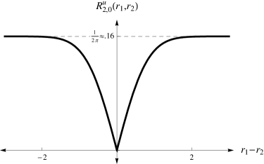
Figure 1: $R^{u}_{2,0}(r_{1},r_{2})$ in the real bulk as a function of $r_{1}-r_{2}$.

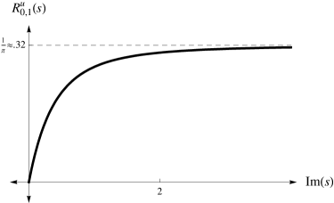
Figure 2: The density of complex eigenvalues in the real bulk as a function of $\mathrm{Im}(s)$.

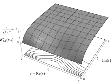
Figure 3: $R^{u}_{1,1}(r,s)$ in the real bulk as a function of $r-\mathrm{Re}(s)$ and $\mathrm{Im}(s)$.

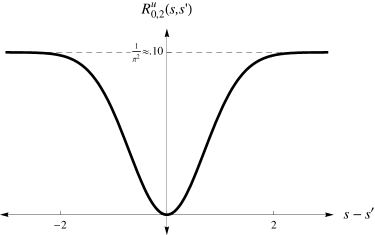
Figure 4: A plot of $R^{u}_{0,2}(s,s^{\prime})$ in the complex bulk as a function of $s-s^{\prime}$

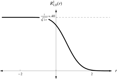
Figure 5: The density of real eigenvalues at the real edge as a function of $r$.

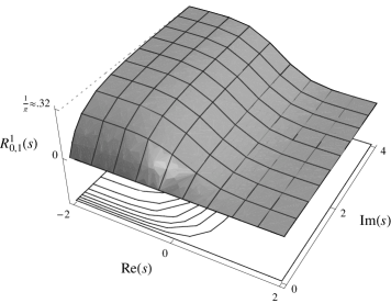
Figure 6: The density of complex eigenvalues at the real edge as a function of $\mathrm{Re}(s)$ and $\mathrm{Im}(s)$.

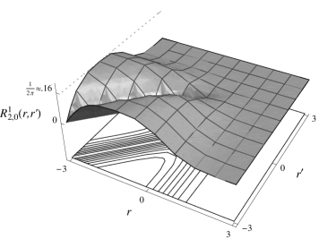
Figure 7: A plot of $R_{2,0}^{1}(r,r^{\prime})$ at the real edge as a function of $r$ and $r^{\prime}$.

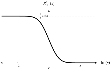
Figure 8: The radial density of eigenvalues (represented here as $R^{i}_{0,1}(s)$) as a function of the radius (given here by $\mathrm{Im}(s)$) at the complex edge.

 

Alexei Borodin
California Institute of Technology
Pasadena, California
email: borodin@caltech.edu

Christopher D. Sinclair
University of Colorado
Boulder, Colorado
email: chris.sinclair@colorado.edu

References

• [1] Garnot Akemann and Eugene Kanzieper. Integrable structure of Ginibre’s ensemble of real random matrices and a pfaffian integration theorem, 2007.
• [2] Z. D. Bai. Circular law. Ann. Probab., 25(1):494–529, 1997.
• [3] Pavel Bleher and Robert Mallison, Jr. Zeros of sections of exponential sums. Int. Math. Res. Not., pages Art. ID 38937, 49, 2006.
• [4] Alexei Borodin and Grigori Olshanski. Representation theory and random point processes. In European Congress of Mathematics, pages 73–94. Eur. Math. Soc., Zürich, 2005.
• [5] A. J. Carpenter, R. S. Varga, and J. Waldvogel. Asymptotics for the zeros of the partial sums of $e^{z}$. I. In Proceedings of the U.S.-Western Europe Regional Conference on Padé Approximants and Related Topics (Boulder, CO, 1988), volume 21, pages 99–120, 1991.
• [6] Shey-Jey Chern and Jeffrey D. Vaaler. The distribution of values of Mahler’s measure. J. Reine Angew. Math., 540:1–47, 2001.
• [7] N. G. de Bruijn. On some multiple integrals involving determinants. J. Indian Math. Soc. (N.S.), 19:133–151 (1956), 1955.
• [8] Alan Edelman. The probability that a random real Gaussian matrix has $k$ real eigenvalues, related distributions, and the circular law. J. Multivariate Anal., 60(2):203–232, 1997.
• [9] Alan Edelman, Eric Kostlan, and Michael Shub. How many eigenvalues of a random matrix are real? J. Amer. Math. Soc., 7(1):247–267, 1994.
• [10] Graham Everest and Thomas Ward. Heights of polynomials and entropy in algebraic dynamics. Universitext. Springer-Verlag London Ltd., London, 1999.
• [11] Peter Forrester and Taro Nagao. Skew orthogonal polynomials and the partly symmetric real Ginibre ensemble. In preparation.
• [12] Peter J. Forrester and Taro Nagao. Eigenvalue statistics of the real Ginibre ensemble. Phys. Rev. Lett., 99, 2007.
• [13] Yan V. Fyodorov and H.-J. Sommers. Random matrices close to Hermitian or unitary: overview of methods and results. J. Phys. A, 36(12):3303–3347, 2003. Random matrix theory.
• [14] Jean Ginibre. Statistical ensembles of complex, quaternion, and real matrices. J. Mathematical Phys., 6:440–449, 1965.
• [15] V. L. Girko. The circular law. Teor. Veroyatnost. i Primenen., 29(4):669–679, 1984.
• [16] Thomas Guhr, Axel Mueller-Groeling, and Hans A. Weidenmueller. Random matrix theories in quantum physics: Common concepts. Physics Reports, 299:189, 1998.
• [17] Eugene Kanzieper and Gernot Akemann. Statistics of real eigenvalues in Ginibre’s ensemble of random real matrices. Physical Review Letters, 95:230201, 2005.
• [18] N. Lehmann and H.-J. Sommers. Eigenvalue statistics of random real matrices. Physical Review Letters, 67:941–944, August 1991.
• [19] Madan Lal Mehta. Random matrices, volume 142 of Pure and Applied Mathematics (Amsterdam). Elsevier/Academic Press, Amsterdam, third edition, 2004.
• [20] Eric M. Rains. Correlation functions for symmetrized increasing subsequences, 2000.
• [21] Christopher D Sinclair. Averages over Ginibre’s ensemble of random real matrices. Int. Math. Res. Not., 2007:1–15, 2007.
• [22] Christopher D. Sinclair. The range of multiplicative functions on $\mathbb{C}[x],\mathbb{R}[x]$ and $\mathbb{Z}[x]$. Proc. London Math. Soc., 96(3):697–737, 2008.
• [23] John R. Stembridge. Nonintersecting paths, Pfaffians, and plane partitions. Adv. Math., 83(1):96–131, 1990.
• [24] T. Tao and V. Vu. Random Matrices: The circular Law. ArXiv e-prints, 708, August 2007.
• [25] N. M. Temme. Uniform asymptotic expansions of the incomplete gamma functions and the incomplete beta function. Math. Comp., 29(132):1109–1114, 1975.
• [26] Craig A. Tracy and Harold Widom. Correlation functions, cluster functions, and spacing distributions for random matrices. J. Statist. Phys., 92(5-6):809–835, 1998.
Refer to caption