Latest inflation model constraints from cosmic microwave background measurements
Abstract
We present an update of cosmological constraints on single-field inflation in light of the Wilkinson Microwave Anisotropy Probe satellite mission five-year results (WMAP5). We find that the cosmic microwave background data are quite consistent with a Harrison-Zel’dovich primordial spectrum with no running and zero tensor amplitude. We find that the three main conclusions of our analysis of the WMAP three-year data (WMAP3) are consistent with the WMAP5 data: (1) the Harrison–Zel’dovich model is within the confidence level contours; (2) there is no evidence for running of the spectral index of scalar perturbations; (3) From the WMAP 5 data alone, potentials of the form are consistent with the data for , and are ruled out for . Furthermore, consistent with our WMAP3 analysis, we find no evidence for primordial tensor perturbations, this time with a confidence upper limit of for the WMAP5 data alone, and for the WMAP5 data taken in combination with the Arcminute Cosmology Bolometer Array (ACBAR).
pacs:
98.80.CqI Introduction
Inflation lrreview is the dominant paradigm for understanding the initial conditions for structure formation and for Cosmic Microwave Background (CMB) temperature anisotropies. In the inflationary scenario, primordial density and gravitational-wave fluctuations are created from quantum fluctuations, “redshifted” beyond the horizon during an early period of superluminal expansion of the universe, then “frozen” Starobinsky:1979ty ; muk81 ; bardeen83 . Perturbations at the surface of last scattering are observable as temperature anisotropies in the CMB, as first detected by the Cosmic Background Explorer satellite. The latest confirmation of the inflationary paradigm has been recently provided by the five-year data from the Wilkinson Microwave Anisotropy Probe (WMAP) satellite wmap5cosm ; wmap5source ; wmap5like ; wmap5ang ; wmap5fore ; wmap5data . The WMAP collaboration has produced new full-sky temperature and polarization maps in five frequency bands from 23 to 94 GHz based on the first five years of the WMAP sky survey. The five-year maps incorporate several improvements in data processing made possible by the additional years of data and by a more complete analysis of the instrument calibration and in-flight beam response. WMAP data support the inflationary model as the mechanism for the generation of super-horizon curvature fluctuations.
The goal of this paper is to make use of the recent WMAP five-year data to discriminate among the various single-field inflationary models. As such, this paper represents an update of our previous analyses wmapping1 ; wmapping2 of the first-year and three-year WMAP data, respectively. The reader is referred to Ref. wmapping2 for a more detailed discussion of the inflationary model space, and for more extensive references.
We compare our results to those reported by the WMAP team in Komatsu et al., wmap5cosm and in Dunkley et al. wmap5like . As first pointed out in Ref. dodelson97 , for single-field inflation models, the relevant parameter space for distinguishing among models is defined by the scalar spectral index , the ratio of tensor to scalar fluctuations , and the running of the scalar spectral index . The Harrison-Zeldovich (H-Z) point () is comfortably within the C.L. contour of Ref. wmap5cosm , and just at the borderline of the C.L. contour of Ref. wmap5like . This small difference appears to be statistically insignificant. In our analysis using the WMAP5 data with slightly different priors than used by the WMAP team (discussed in Sec. III) we find that marginalizing over all parameters except and in the WMAP5 data, the likelihood of the H-Z point , is 0.0988, corresponding to exclusion of the H-Z model with confidence level of . Marginalizing over all parameters except (i.e., the single-parameter confidence limits on for the same parameter set), the likelihood of the point is 0.4226, corresponding to exclusion of the scale-invariant spectrum with a confidence level of . These figures are highly dependent on our choice of priors: if we use a six-parameter fit with a prior of , the likelihood of the point is , corresponding to the exclusion of the scale-invariant spectrum with a confidence level of . (In all cases, the maximum likelihood is normalized to unity.) Our conclusion is that the H-Z model is not preferred, but neither is it strongly disfavored.
The paper is organized as follows: In Sec. II we will quickly review single-field inflation models and their observables. In Sec. III we define the inflationary model space as a function of the slow-roll parameters and . In Sec. IV we describe our analysis method as well as our results. Since a study of the implications of the WMAP5 data for single field models of inflation has been already performed by the WMAP collaboration themselves wmap5cosm , we will also specify the differences between our analysis and theirs. In Sec. V we present our conclusions.
II Single-field inflation and the inflationary observables
Inflation not only explains the large-scale homogeneity of the universe, but also provide a mechanism for explaining the observed level of inhomogeneity as well. During inflation, quantum fluctuations on small scales are quickly redshifted to scales much larger than the horizon size, where they are “frozen” as perturbations in the background metric. The metric perturbations created during inflation are of two types: scalar, or curvature perturbations, which couple to the stress-energy of matter in the universe and form the “seeds” for structure formation, and tensor, or gravitational-wave perturbations, which do not couple to matter. Both scalar and tensor perturbations contribute to CMB anisotropies. Scalar fluctuations can also be interpreted as fluctuations in the density of the matter in the universe. Scalar fluctuations can be quantitatively characterized by the comoving curvature perturbation . As long as slow-roll is attained, the curvature (scalar) perturbation at horizon crossing can be shown to be lrreview
| (1) |
Here, denotes the slow-rolling scalar field dominating the energy density of the Universe during inflation, the so-called inflaton, is the Hubble rate and GeV is the Planck scale. The slow roll approximation is consistent if both the slope and curvature of the inflaton potential are small (in Planckian units), . In this case the slow-roll parameter can be expressed in terms of the potential as
| (2) |
We will also need in the following a second “slow-roll parameter” defined by
| (3) |
Slow roll is then a consistent approximation for .
The fluctuation power spectrum is, in general, a function of wavenumber , and is evaluated when a given mode crosses outside the horizon during inflation, . Outside the horizon, modes do not evolve, so the amplitude of the mode when it crosses back inside the horizon during a later radiation- or matter-dominated epoch is just its value when it left the horizon during inflation. Instead of specifying the fluctuation amplitude directly as a function of , it is convenient to specify it as a function of the number of e-folds before the end of inflation at which a mode crossed outside the horizon.
The scalar spectral index for is defined by
| (4) |
so that a scale-invariant spectrum, in which modes have constant amplitude at horizon crossing, is characterized by .
The power spectrum of tensor fluctuation modes and the corresponding tensor spectral index is given by lrreview
| (5) |
The ratio of tensor-to-scalar modes is then , so that tensor modes are negligible for . In the limit of slow roll, the spectral indices and vary slowly or not at all with scale. We can write the spectral indices and to lowest order in terms of the slow roll parameters and as
| (6) |
The tensor/scalar ratio is frequently expressed as a quantity , which is conventionally normalized as
| (7) |
The tensor spectral index is not an independent parameter, but is proportional to the tensor/scalar ratio, given to lowest order in slow roll by . This is known as the consistency relation for inflation. A given inflation model can therefore be described to lowest order in slow roll by three independent parameters: , , and . If we wish to include higher-order effects, we would have to include a fourth parameter describing the running of the scalar spectral index, .
III Analysis and Results
The method we adopt is based on the publicly available Markov Chain Monte Carlo (MCMC) package cosmomc Lewis:2002ah . We sample the following eight-dimensional set of cosmological parameters, adopting flat priors on them: the physical baryon and CDM densities, and , the ratio of the sound horizon to the angular diameter distance at decoupling, , the scalar spectral index, its running, and the overall normalization of the spectrum, , and at some pivot scale (either Mpc-1 or Mpc-1), the tensor contribution , and, finally, the optical depth to reionization, . Furthermore, we consider purely adiabatic initial conditions, we impose spatial flatness, and we use the inflation consistency relation to fix the value of the tensor spectral index . We also restrict our analysis to the case of three massless neutrino families; introducing a neutrino mass in agreement with current neutrino oscillation data does not change our results in a significant way.
We include the five-year data wmap5cosm (temperature and polarization) with the routine for computing the likelihood supplied by the WMAP team and available at the LAMBDA web site http://lambda.gsfc.nasa.gov/. We also perform an analysis based on the WMAP five-year data in combination with results from the Arcminute Cosmology Bolometer Array (ACBAR) Reichardt:2008ay . The MCMC convergence diagnostic is done on chains though the Gelman and Rubin “variance of chain mean”“mean of chain variances” statistic for each parameter. Our 1D and 2D constraints are obtained after marginalization over the remaining “nuisance” parameters, again using the programs included in the cosmomc package. Furthermore, we make use of the HST measurement of the Hubble parameter hst by multiplying the likelihood by a Gaussian likelihood function centered around and with a standard deviation . Finally, we include a top-hat prior on the age of the universe: Gyrs. We perform the analysis in two ways: first, we constrain parameters with a prior assumption of , i.e., an exact power-law perturbation spectrum, and second, with a free parameter in the MCMC. We include lensing in the calculation, and marginalize over the Sunyaev-Zel’dovich amplitude using the WMAP V-band template.
All fits are performed at a pivot scale of , which is different from our previous analysis and the analysis of Dunkley et al. and Komatsu et al., all of which are normalized to a pivot scale of . The reason for the different choice of pivot scale is to mitigate the parameter degeneracy between and Cortes:2007ak , which significantly improves convergence of the MCMC code. In the case of , the choice of pivot scale has no effect on the spectral index , since a change of pivot affects only the normalization:
| (8) |
However, the change of pivot results in a rescaling of the tensor/scalar ratio which is dependent on and , since
| (9) |
and therefore, using the consistency relation ,
| (10) |
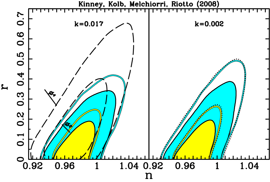
Figure 1 shows % and % confidence limits on and in the case of a no-running prior, . Clearly the choice of the pivot scale makes very little difference in this case (and since it is just a normalization for , no difference at all in the case.)
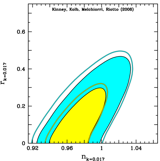
In Fig. 2 we show the % and % confidence limits on and in the case where we allow running of the spectrum as a free parameter. Again the WMAP5 alone data correspond to the open contours and WMAP5 + ACBAR to the filled contours.
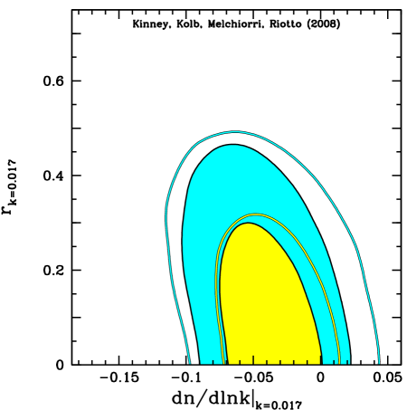
Finally in Fig. 3 we show the % and % confidence limits on as a function of and as a function of .
IV Conclusions
In this paper we presented an analysis of the recent WMAP five-year data set with an emphasis on parameters relevant for distinguishing among the various possible models for inflation. This analysis is an update to our similar analysis of the WMAP three-year data set wmapping2 . In that analysis, we reached three main conclusions, which are either unchanged or slightly strengthened by the new data: (1) the Harrison–Zel’dovich model is within the confidence level contour. We find that marginalizing over all parameters except and in the WMAP5 data, the likelihood of the H-Z point , is 0.0988, corresponding to exclusion of the H-Z model with confidence level of . Marginalizing over all parameters except (i.e., the single-parameter confidence limits on for the same parameter set), the likelihood of the point is , corresponding to exclusion of the scale-invariant spectrum with a confidence level of . These figures are highly dependent on our choice of priors: if we use a six-parameter fit with a prior of , the likelihood of the point is , corresponding to the exclusion of the scale-invariant spectrum with a confidence level of . (In all cases, the likelihood is calculated as the marginalized posterior probability, with the best-fit point normalized to unity. The confidence level is calculated from the likelihood assuming a Gaussian error distribution.) (2) There is no evidence for running of the spectral index of scalar perturbations. Figure 3 shows likelihood contours for relative to the parameters and , calculated at a pivot scale of to minimize parameter degeneracies, showing that the case of a pure power-law spectrum is fully consistent with all data sets. (3) Potentials of the form are consistent with the data for , and are ruled out by the WMAP five-year data alone for . This is a stronger conclusion that was possible with the WMAP three-year data, which was marginally consistent with at a C.L. We find no evidence for a nonzero tensor/scalar ratio, with a C.L. upper limit of for the WMAP five-year data alone, and for WMAP in combination with ACBAR. Our results are consistent with the results of Peiris and Easther in Ref. Peiris:2008be .
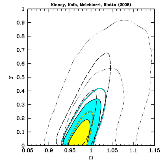
Finally, we illustrate the consistency of CMB determinations of and over the years in Fig. 4. The pre-WMAP status is well described by the combination of the COBE COBE , BOOMERANG Netterfield01 , MAXIMA Hanany00 , DASI Halverson01 , and CBI Pearson02 data sets. This pre-WMAP analysis includes also a prior on the optical depth . As illustrated by the figure, higher precision data prefers , but is not strongly disfavored.
Acknowledgements.
We acknowledge support provided by the Center for Computational Research at the University at Buffalo. WHK is supported in part by the National Science Foundation under grant NSF-PHY-0456777. This research was supported in part by the Department of Energy and the European Community’s Research Training Networks under contracts MRTN-CT-2004-503369, MRTN-CT-2006-035505. This research has been supported by ASI contract I/016/07/0 “COFIS.” We thank Joanna Dunkley and Eichiro Komatsu for helpful conversations.References
- (1) For reviews, see D. H. Lyth and A. Riotto, Phys. Rept. 314, 1 (1999); W. H. Kinney, arXiv:astro-ph/0301448.
- (2) A. A. Starobinsky, JETP Lett. 30, 682 (1979) [Pisma Zh. Eksp. Teor. Fiz. 30, 719 (1979)].
- (3) V. F. Mukhanov and G. V. Chibisov, JETP Lett. 33, 532 (1981).
- (4) J. M. Bardeen, P. J. Steinhardt, and M. S. Turner, Phys. Rev. D 28, 679 (1983).
- (5) E. Komatsu et al., arXiv:0803.0547 [astro-ph].
- (6) E. L. Wright et al., arXiv:0803.0577 [astro-ph].
- (7) J. Dunkley et al., arXiv:0803.0586 [astro-ph].
- (8) M. R. Nolta et al., arXiv:0803.0593 [astro-ph].
- (9) B. Gold et al., arXiv:0803.0715 [astro-ph].
- (10) G. Hinshaw et al., arXiv:0803.0732 [astro-ph].
- (11) W. H. Kinney, E. W. Kolb, A. Melchiorri and A. Riotto, Phys. Rev. D 69, 103516 (2004).
- (12) W. H. Kinney, E. W. Kolb, A. Melchiorri and A. Riotto, Phys. Rev. D 74, 023502 (2006).
- (13) S. Dodelson, W. H. Kinney, and E. W. Kolb, Phys. Rev. D 56, 3207 (1997).
- (14) A. Lewis and S. Bridle, Phys. Rev. D 66, 103511 (2002) (Available from http://cosmologist.info.)
- (15) W. L. Freedman et al., Astrophys. J. 553, 47 (2001).
- (16) C. L. Reichardt et al., arXiv:0801.1491 [astro-ph].
- (17) M. Cortes, A. R. Liddle and P. Mukherjee, Phys. Rev. D 75, 083520 (2007).
- (18) H. V. Peiris and R. Easther, arXiv:0805.2154 [astro-ph].
- (19) C. L. Bennett, et al., Astrophys. J. Lett., 464 L1, 1996.
- (20) C. B. Netterfield et al., Astrophys. J. , 571, 604, (2002).
- (21) S. Hanany et al., Astrophys. J. , 545, L5, (2000).
- (22) N. W. Halverson et al., Astrophys. J. , 568, 38, (2002).
- (23) J. L. Sievers et al., (2002), eprint astro-ph/0205387
- (24) T. J. Pearson et al., (2002), eprint astro-ph/0205388.


