QCD Sum Rules Study of the Semileptonic $B_{s}(B^{\pm})(B^{0})\rightarrow D_{s}[1968](D^{0})(D^{\pm})l\nu$ Decays

Abstract

The form factors of the semileptonic $B_{q}\rightarrow D_{q}(J^{P}=0^{-})\ell\nu$ with $q=s,u,d$ transitions are calculated in the framework of three point QCD sum rules. Using the $q^{2}$ dependencies of the relevant form factors, the total decay width and the branching ratio for these decays are also evaluated. A comparison of our results for the form factors of $B\rightarrow D\ell\nu$ with the lattice QCD predictions within heavy quark effective theory and zero recoil limit is presented. Our results of the branching ratio are in good agreement with the constituent quark meson model for ($q=s,u,d$) and experiment for ($q=u,d$). The result of branching ratio for $B_{s}\rightarrow D_{s}(1968)\ell\nu$ indicates that this transition can also be detected at LHC in the near future.

1 Introduction

The pseudoscalar $B_{q}$ meson decays are very promising tools to constrain the Standard Model (SM) parameters, explore heavy quark dynamics and search for new physics. The semileptonic decays of heavy flavored mesons are also useful for determination of the elements of the Cabibbo-Kobayashi-Maskawa (CKM) matrix, leptonic decay constants as well as the origin of the CP violation. Neutral $B_{s}^{0}$ and $B_{d}^{0}$ meson decays are interesting to study CP violation.

When LHC begins operation, an abundant number of $B_{q}$ mesons will be produced. This will provide a real possibility for studying the properties of the $B_{q}$ mesons and their various decay channels. Some possible decay channels of $B_{q}$ mesons are their semileptonic decays to $D_{q}l\nu$ . The $B_{q}\rightarrow D_{q}\ell\nu$ transitions occur via the $b\rightarrow c$ transition with s, d or u as spectator quarks. The most common decay mode of B mesons is clearly $b\rightarrow c$ transition, since it is the most dominant transition among the b quark decays. The semileptonic $B_{q}\rightarrow D_{q}\ell\nu$ decays are interesting because they could play a fundamental role in probing new physics charged Higgs contributions in low energy observables. Moreover, they open a window onto the strong interactions of the constituent quarks of the pseudoscalar $D_{s}$ meson and could give useful information about the structure of this meson (for a discussion about the nature of $D_{sJ}$ mesons and their quark content see [1, 2]). Analysis of the $D_{s_{0}}(2317)\rightarrow D_{s}^{\ast}\gamma$, $D_{sJ}(2460)\rightarrow D_{s}^{\ast}\gamma$ and $D_{sJ}(2460)\rightarrow D_{s_{0}}(2317)\gamma$ indicates that the quark content of these mesons is probably $\overline{c}s$ [3].

The long distance dynamics of such type transitions are parameterized in terms of some form factors, which are related to the structure of the initial and final meson states. For calculation of these form factors which play fundamental role in the analysis of these transitions, some nonperturbative approaches are needed. Among the existing nonperturbative methods, QCD sum rules has received especial attention, because this approach is based on the fundamental QCD Lagrangian. There are two kinds of QCD sum rule approaches, three point and light cone QCD. In three point QCD sum rules, the perturbative part of the correlation function is expanded in terms of operators having different mass dimensions with the help of the operator product expansion (OPE). In light cone QCD, the distribution amplitudes (DA’s) of the particles expanding in terms of different twists are used [4, 5, 6]. This method has been applied successfully for wide variety of problems [7, 8, 9, 10, 11] (for a review see also [12]). In present work, we describe the semileptonic $B_{q}\rightarrow D_{q}\ell\nu$ decays by calculating the relevant form factors in the framework of the three point QCD sum rules approach. Note that, the form factors of $B\rightarrow D\ell\nu$ have been calculated in lattice QCD [13, 14, 15, 16] and the subleading Isgur-Wise form factor is computed in QCD sum rules and its application for the $B\rightarrow D\ell\nu$ decay is shown in [17, 18](for similar previous works see also [19, 20, 21] ). Moreover, the $B_{q}\rightarrow D_{q}\ell\nu$ transitions have been studied in the constituent quark meson (CQM) model for $q=s,u,d$ in [22] and for $q=u,d$, the experimental results can be found in [23].

This paper is organized as follows: In section II, we calculate the sum rules for the two form factors relevant to these transitions. Section III is devoted with the numerical analysis, conclusion, discussion and comparison of our results for the form factors and branching ratios with those of the other phenomenological model, lattice QCD and experiment.

2 Sum rules for the $B_{q}\rightarrow D_{q}\ell\nu$ transition form factors

In the quark level, the $B_{q}\rightarrow D_{q}\ell\nu$ transitions proceed by the $b\rightarrow c$ transition (see Fig. 1).

Figure 1: $B_{q}\rightarrow D_{q}\ell\nu$ transitions at tree level

The matrix element for these transitions at the quark level can be written as:

$$M_{q}=\frac{G_{F}}{\sqrt{2}}V_{cb}~{}\overline{\nu}~{}\gamma_{\mu}(1-\gamma_{5})l~{}\overline{c}~{}\gamma_{\mu}(1-\gamma_{5})b.$$ (1)

To obtain the matrix elements for $B_{q}\rightarrow D_{q}\ell\nu$ decays, we need to sandwich Eq. (1) between initial and final meson states, so the amplitude of these decays gets the following form:

$$M=\frac{G_{F}}{\sqrt{2}}V_{cb}~{}\overline{\nu}~{}\gamma_{\mu}(1-\gamma_{5})l<D_{q}(p^{\prime})\mid~{}\overline{c}~{}\gamma_{\mu}(1-\gamma_{5})b\mid B_{q}(p)>.$$ (2)

Our aim is to calculate the matrix elements $<D_{q}(p^{\prime})\mid\overline{c}\gamma_{\mu}(1-\gamma_{5})b\mid B_{q}(p)>$ appearing in Eq. (2). Because of parity and Lorentz invariance the axial vector part of transition current, $~{}\overline{c}~{}\gamma_{\mu}(1-\gamma_{5})b~{}$, does not have any contribution to the matrix element considered above, so the contribution comes only from the vector part of the transition current. Considering the parity and Lorentz invariances, one can parameterize this matrix element in terms of the form factors in the following way:

$$<D_{q}(p^{\prime})\mid\overline{c}\gamma_{\mu}b\mid B_{q}(p)>=f_{1}(q^{2})P_{\mu}+f_{2}(q^{2})q_{\mu},$$ (3)

where $f_{1}(q^{2})$, $f_{2}(q^{2})$ are the transition form factors and $P_{\mu}=(p+p^{\prime})_{\mu}$, $q_{\mu}=(p-p^{\prime})_{\mu}$.

From the general philosophy of QCD sum rules method, in order to calculate the form factors we consider the following correlator:

$$\Pi_{\mu}(p^{2},p^{\prime 2},q^{2})=i^{2}\int d^{4}xd^{4}ye^{-ipx}e^{ip^{\prime}y}<0\mid T[J_{D_{q}}(y)J_{\mu}^{t}(0)J_{B_{q}}(x)]\mid 0>,$$ (4)

where $J_{D_{q}}(y)=\overline{c}\gamma_{5}q$ and $J_{B_{q}}(x)=\overline{b}\gamma_{5}q$ are the interpolating currents of the $D_{q}$ and $B_{q}$, respectively and $J_{\mu}^{t}(0)=~{}\overline{c}\gamma_{\mu}b$ is the transition current.

To calculate the phenomenological or physical part of the correlator given in Eq. (4), two complete sets of intermediate states with the same quantum numbers as the currents $J_{D_{q}}$ and $J_{B_{q}}$ respectively are inserted. As a result of this procedure, we get the following representation of the above-mentioned correlator:

$$\Pi_{\mu} = \frac{<0\mid J_{D_{q}}(0)\mid D_{q}(p^{\prime})><D_{q}(p^{\prime})\mid J_{\mu}^{t}(0)\mid B_{q}(p)><B_{q}(p)\mid J_{q}(0)\mid 0>}{(p^{\prime 2}-m_{D_{q}}^{2})(p^{2}-m_{B_{{}_{q}}}^{2})}$$ (5)

$$+ \cdots,$$

where $\cdots$ represents the contributions coming from higher states and continuum. The following matrix elements in Eq. (5) are defined in the standard way as:

$$<0\mid J_{D_{q}}\mid D_{q}(p^{\prime})>=-i\frac{f_{D_{q}}m_{D_{q}}^{2}}{m_{c}+m_{q}},$$

$$<B_{q}(p)\mid J_{B_{q}}\mid 0>=-i\frac{f_{B_{q}}m_{B_{q}}^{2}}{m_{b}+m_{q}},$$ (6)

where $f_{D_{q}}$ and $f_{B_{q}}$ are the leptonic decay constants of $D_{q}$ and $B_{q}$ mesons, respectively. Using Eq. (3) and Eq. (2), Eq. (5) can be written in hadronic language as:

$$\Pi_{\mu}(p^{2},p^{\prime 2},q^{2})=\Pi_{1}(p^{2},p^{\prime 2},q^{2})P_{\mu}+\Pi_{2}(p^{2},p^{\prime 2},q^{2})q_{\mu},$$ (7)

Where,

$$\Pi_{1}(p^{2},p^{\prime 2},q^{2}) = -\frac{1}{(p^{\prime 2}-m_{D_{q}}^{2})(p^{2}-m_{B_{{}_{q}}}^{2})}\frac{f_{D_{q}}m_{D_{q}}^{2}}{m_{c}+m_{q}}\frac{f_{B_{q}}m_{B_{q}}^{2}}{m_{b}+m_{q}}f_{1}(q^{2})$$

$$+$$ excited states,

$$\Pi_{2}(p^{2},p^{\prime 2},q^{2}) = -\frac{1}{(p^{\prime 2}-m_{D_{q}}^{2})(p^{2}-m_{B_{{}_{q}}}^{2})}\frac{f_{D_{q}}m_{D_{q}}^{2}}{m_{c}+m_{q}}\frac{f_{B_{q}}m_{B_{q}}^{2}}{m_{b}+m_{q}}f_{2}(q^{2})$$ (8)

$$+$$ excited states.

Now, let calculate the theoretical part (QCD side) of the correlation function $\Pi_{\mu}(p^{2},p^{\prime 2},q^{2})$ in quark and gluon languages with the help of the operator product expansion(OPE) in the deep Euclidean region $p^{2}\ll(m_{b}+m_{q})^{2}$ and $p^{\prime 2}\ll(m_{c}+m_{q})^{2}$. The correlator is written in terms of the perturbative and nonperturbative parts as:

$$\Pi_{\mu}(p^{2},p^{\prime 2},q^{2}) = \bigg{[}\Pi^{per}_{1}(p^{2},p^{\prime 2},q^{2})+\Pi^{non-per}_{1}(p^{2},p^{\prime 2},q^{2})\bigg{]}P_{\mu}$$ (9)

$$+ \bigg{[}\Pi^{per}_{2}(p^{2},p^{\prime 2},q^{2})+\Pi^{non-per}_{2}(p^{2},p^{\prime 2},q^{2})\bigg{]}q_{\mu}.$$

To obtain the sum rules for the form factors, the two different representations of $\Pi_{\mu}(p^{2},p^{\prime 2},q^{2})$ are equated. The theoretical part of the correlator is calculated by means of OPE, and up to operators having dimension $d=5$, it is determined by the bare-loop (Fig. 2a) and the power correction diagrams from the operators with $d=3$, $<\overline{q}q>$, $d=4$, $m_{s}<\overline{q}q>$, $d=5$, $m_{0}^{2}<\overline{q}q>$ (Fig. 2b, 2c, 2d).

Figure 2: Diagrams for bare-loop and power corrections (light quark condensates)

In calculating the bare-loop contribution, we first write the double dispersion representation for the coefficients of corresponding Lorentz structures appearing in the correlation function as:

$$\Pi_{i}^{per}=-\frac{1}{(2\pi)^{2}}\int ds\int ds^{\prime}\frac{\rho_{i}(s,s^{\prime},q^{2})}{(s-p^{2})(s^{\prime}-p^{\prime 2})}+\textrm{ subtraction terms}.$$ (10)

The spectral densities $\rho_{i}(s,s^{\prime},q^{2})$ can be calculated from the usual Feynman integral (bare loop diagram in Fig. 2a) with the help of Cutkosky rules, i.e., by replacing the quark propagators with Dirac delta functions: $\frac{1}{p^{2}-m^{2}}\rightarrow-2\pi\delta(p^{2}-m^{2}),$ which implies that all quarks are real. After some straightforward calculations for the spectral densities corresponding to $P_{\mu}$ and $q_{\mu}$ we obtain:

$$\rho_{1}(s,s^{\prime},q^{2}) = N_{c}I_{0}(s,s^{\prime},q^{2})[2m_{b}m_{q}+2m_{c}m_{q}-4m_{q}^{2}$$

$$- 2A(\Delta+m_{b}^{2}-m_{q}^{2})-(A+B)u^{\prime}-2B(\Delta^{\prime}+m_{c}^{2}-m_{q}^{2})],$$

$$\rho_{2}(s,s^{\prime},q^{2}) = N_{c}I_{0}(s,s^{\prime},q^{2})[-2m_{b}m_{q}+2m_{c}m_{q}+2A(\Delta+m_{b}^{2}-m_{q}^{2})$$ (11)

$$+ (B-A)u^{\prime}-2B(\Delta^{\prime}+m_{c}^{2}-m_{q}^{2})],$$

where

$$I_{0}(s,s^{\prime},q^{2}) = \frac{1}{4\lambda^{1/2}(s,s^{\prime},q^{2})},$$

$$\lambda(s,s^{\prime},q^{2}) = s^{2}+s^{\prime 2}+q^{4}-2sq^{2}-2s^{\prime}q^{2}-2ss^{\prime},$$

$$\Delta^{\prime} = (s^{\prime}-m_{c}^{2}+m_{q}^{2}),$$

$$\Delta = (s-m_{b}^{2}+m_{q}^{2}),$$

$$A = \frac{1}{\lambda(s,s^{\prime},q^{2})}[2s^{\prime}\Delta-\Delta^{\prime}u],$$

$$B = \frac{1}{\lambda(s,s^{\prime},q^{2})}[2s\Delta^{\prime}-\Delta u],$$

$$u = s+s^{\prime}-q^{2},$$

$$u^{\prime} = 2[m_{b}m_{c}-(m_{b}+m_{c})m_{q}+m_{q}^{2}].$$

In Eq. (2) $N_{c}=3$ is the number of colors. The integration region for the perturbative contribution in Eq. (10) is determined from the condition that arguments of the three $\delta$ functions must vanish simultaneously. The physical region in $s$ and $s^{\prime}$ plane is described by the following inequalities:

$$-1\leq\frac{2ss^{\prime}+(s+s^{\prime}-q^{2})(m_{b}^{2}-s-m_{q}^{2})+(m_{q}^{2}-m_{c}^{2})2s}{\lambda^{1/2}(m_{b}^{2},s,m_{q}^{2})\lambda^{1/2}(s,s^{\prime},q^{2})}\leq+1.$$ (13)

From the above equation, it is easy to calculate the lower bound of integration over $s^{\prime}$ as a function of s. (i.e., $s^{\prime}=f(s)$).

For the contribution of power corrections, i.e., the contributions of operators with dimensions $d=3$, $4$ and $5$ (diagrams in Fig. 2b, 2c ,2d), we obtain the following results:

$$\Pi^{non-per}_{1} = -\frac{1}{2r^{\prime}r}<\overline{q}q>(m_{b}+m_{c})+\frac{m_{q}}{4}<\overline{q}q>\left[\frac{m_{b}m_{c}+m_{c}^{2}}{r^{\prime 2}r}+\frac{m_{b}^{2}+m_{b}m_{c}}{r^{\prime}r^{2}}\right]$$

$$+ \frac{1}{2}<\overline{q}q>(-m_{q}^{2}+\frac{1}{2}m_{0}^{2})\left\{\frac{m_{b}m_{c}^{2}+m_{c}^{3}}{r^{\prime 3}r}+\frac{1}{2}\frac{(m_{c}+m_{b})(-q^{2}+m_{b}^{2}+m_{c}^{2})}{r^{\prime 2}r^{2}}\right.$$

$$+ \left.\frac{1}{2}(m_{c}+m_{b})\left[\frac{1}{r^{\prime 2}r}+\frac{1}{r^{\prime}r^{2}}\right]+\frac{m_{b}^{3}+m_{b}^{2}m_{c}}{r^{\prime}r^{3}}\right\}$$

$$+ <\overline{q}q>\frac{m_{0}^{2}}{48}\frac{(3m_{b}+m_{c})}{r^{\prime}r^{2}}+<\overline{q}q>\frac{m_{0}^{2}}{48}\left\{\frac{-4(m_{b}+2m_{c})}{r^{\prime 2}r}-\frac{(2m_{b}+m_{c})}{r^{\prime}r^{2}}\right.$$

$$+ \left.\frac{(-m_{b}^{3}+m_{b}^{2}m_{c}+m_{b}m_{c}^{2}-m_{c}^{3}+m_{b}q^{2}+m_{c}q^{2})}{r^{\prime 2}r^{2}}\right\},$$

$$\Pi^{non-per}_{2} = \frac{1}{2r^{\prime}r}<\overline{q}q>(m_{b}-m_{c})-\frac{m_{q}}{4}<\overline{q}q>\left[\frac{m_{b}m_{c}-m_{c}^{2}}{r^{\prime 2}r}+\frac{m_{b}^{2}-m_{b}m_{c}}{r^{\prime}r^{2}}\right]$$ (14)

$$+ \frac{1}{2}<\overline{q}q>(-m_{q}^{2}+\frac{1}{2}m_{0}^{2})\left\{\frac{m_{b}m_{c}^{2}-m_{c}^{3}}{r^{\prime 3}r}+\frac{1}{2}\frac{(m_{c}-m_{b})(-q^{2}+m_{b}^{2}+m_{c}^{2})}{r^{\prime 2}r^{2}}\right.$$

$$+ \left.\frac{1}{2}(m_{c}-m_{b})\left[\frac{1}{r^{\prime 2}r}+\frac{1}{r^{\prime}r^{2}}\right]-\frac{m_{b}^{3}-m_{b}^{2}m_{c}}{r^{\prime}r^{3}}\right\}$$

$$- <\overline{q}q>\frac{m_{0}^{2}}{48}\frac{(3m_{b}-m_{c})}{r^{\prime}r^{2}}+<\overline{q}q>\frac{m_{0}^{2}}{48}\left\{\frac{2(2m_{b}-m_{c})}{r^{\prime 2}r}-\frac{m_{c}}{r^{\prime}r^{2}}\right.$$

$$+ \left.\frac{(m_{b}^{3}-3m_{b}^{2}m_{c}+3m_{b}m_{c}^{2}-m_{c}^{3}-m_{b}q^{2}+m_{c}q^{2})}{r^{\prime 2}r^{2}}\right\},$$

where $r=p^{2}-m_{b}^{2},r^{\prime}=p^{\prime 2}-m_{c}^{2}$.

The QCD sum rules for the form factors $f_{1}(q^{2})$ and $f_{2}(q^{2})$ are obtained by equating the phenomenological and QCD parts of the correlator and applying double Borel transformations with respect to the variables $p^{2}$ and $p^{\prime 2}$ ($p^{2}\rightarrow M_{1}^{2},p^{\prime 2}\rightarrow M_{2}^{2}$) in order to suppress the contributions of higher states and continuum:

$$f_{i}(q^{2}) = -\frac{(m_{b}+m_{q})}{f_{B_{q}}m_{B_{q}}^{2}}\frac{(m_{c}+m_{q})}{f_{D_{q}}m^{2}_{D_{q}}}e^{m_{B_{q}}^{2}/M_{1}^{2}}e^{m_{D_{q}}^{2}/M_{2}^{2}}$$ (15)

$$\bigg{\{}-\frac{1}{(2\pi)^{2}}\int_{(m_{b}+m_{q})^{2}}^{s_{0}}ds\int_{f(s)}^{s_{0}^{\prime}}ds^{\prime}\rho_{i}(s,s^{\prime},q^{2})e^{-s/M_{1}^{2}}e^{-s^{\prime}/M_{2}^{2}}$$

$$+\emph{B}(M_{1}^{2})\emph{B}(M_{2}^{2})\Pi^{non-per}_{i}\bigg{\}},$$

where $i=1,2$ and $\emph{B}(M_{1}^{2})\emph{B}(M_{2}^{2})$ denotes the double Borel transformation operator. In Eq. (15), in order to subtract the contributions of the higher states and continuum, the quark-hadron duality assumption is used, i.e., it is assumed that

$$\rho^{higherstates}(s,s^{\prime})=\rho^{OPE}(s,s^{\prime})\theta(s-s_{0})\theta(s^{\prime}-s^{\prime}_{0}).$$ (16)

In calculations, the following rule for double Borel transformations is also used:

$$\hat{B}\frac{1}{r^{m}}\frac{1}{r^{\prime n}}\rightarrow(-1)^{m+n}\frac{1}{\Gamma(m)}\frac{1}{\Gamma(n)}e^{-m_{b}^{2}/M_{1}^{2}}e^{-m_{c}^{2}/M_{2}^{2}}\frac{1}{(M_{1}^{2})^{m-1}(M_{2}^{2})^{n-1}}.$$ (17)

3 Numerical analysis

The sum rules expressions for the form factors $f_{1}(q^{2})$ and $f_{2}(q^{2})$ show that the condensates, leptonic decay constants of $B_{q}$ and $D_{q}$ mesons, continuum thresholds $s_{0}$ and $s^{\prime}_{0}$ and Borel parameters $M_{1}^{2}$ and $M_{2}^{2}$ are the main input parameters. In further numerical analysis, we choose the value of the condensates at a fixed renormalization scale of about $1$ GeV [24]: $<\overline{d}d>=<\overline{u}u>=-(240\pm 10~{}MeV)^{3}$, $<\overline{s}s>=(0.8\pm 0.2)<\overline{u}u>$ and $m_{0}^{2}=0.8\pm 0.2~{}GeV^{2}$. The experimental values for the mass of the mesons, $m_{D_{s}}=1968.2\pm 0.5~{}MeV$, $m_{D_{d}}(m_{D^{\pm}})=1869.3\pm 0.4~{}MeV$, $m_{D_{u}}(m_{D^{0}})=1864.5\pm 0.4~{}MeV$ $m_{B_{s}}=5367.5\pm 1.8~{}MeV$, $m_{B_{d}}(m_{B^{0}})=5279.4\pm 0.5~{}MeV$ and $m_{B_{u}}(m_{B^{\pm}})=5279.0\pm 0.5~{}MeV$ [23] are used. For the value of the leptonic decay constants and quark masses, we use the following values in two sets: In set 1, we use the results obtained from two-point QCD sum rules analysis: $f_{B_{s}}=209\pm 38~{}MeV$ [12], $f_{D_{s}}=294\pm 27~{}MeV$ [3], $f_{B_{d}}=f_{B_{u}}=140\pm 10~{}MeV$ [26] and $f_{D_{d}}=f_{D_{u}}=170\pm 20~{}MeV$ [26]. The quark masses are taken to be $m_{c}(\mu=m_{c})=1.275\pm 0.015~{}GeV$, $m_{s}(1~{}GeV)\simeq 142~{}MeV$ [25], $m_{d}(1~{}GeV)\simeq 5~{}MeV$, $m_{u}(1~{}GeV)\simeq 1.5~{}MeV$ and $m_{b}=(4.7\pm 0.1)~{}GeV$ [24]. In set 2, the recent experimental values $f_{D_{s}}=274\pm 13\pm 7~{}MeV$ [27], $f_{D^{+}}=222.6\pm 16.7^{+2.8}_{-3.4}~{}MeV$ [28], $f_{B^{+}}=176^{+28+20}_{-23-19}~{}MeV$ [23] and lattice prediction for $f_{B_{s}}=206\pm 10~{}MeV$ [29] are used. For heavy quark masses $m_{c}=1.25\pm 0.09~{}GeV$ and $m_{b}=4.7\pm 0.07~{}GeV$ [23] and for light quark masses the values at the scale $\mu=1GeV$ (the same as set 1) are considered. The continuum threshold parameters $s_{0}$ and $s_{0}^{\prime}$ are also determined from the two-point QCD sum rules: $s_{0}=(35\pm 2)~{}GeV^{2}$ [30] and $s_{0}^{\prime}=6~{}GeV^{2}$ [3]. The Borel parameters $M_{1}^{2}$ and $M_{2}^{2}$ are auxiliary quantities and therefore the results of physical quantities should not depend on them. In QCD sum rules method, OPE is truncated at some finite order, leaving a residual dependence on the Borel parameters. For this reason, working regions for the Borel parameters should be chosen such that in these regions form factors are practically independent of them. The working regions for the Borel parameters $M_{1}^{2}$ and $M_{2}^{2}$ can be determined by requiring that, on the one side, the continuum contribution should be small, and on the other side, the contribution of the operator with the highest dimension should be small. As a result of the above-mentioned requirements, the working regions are determined to be $10~{}GeV^{2}<M_{1}^{2}<22~{}GeV^{2}$ and $4~{}GeV^{2}<M_{2}^{2}<10~{}GeV^{2}$.

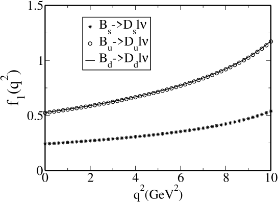
Figure 3: The dependence of $f_{1}$ on $q^{2}$ at $M_{1}^{2}=17~{}GeV^{2}$, $M_{2}^{2}=6~{}GeV^{2}$, $s_{0}=35~{}GeV^{2}$, $s_{0}^{\prime}=6~{}GeV^{2}$ and set1.

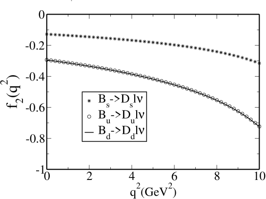
Figure 4: The dependence of $f_{2}$ on $q^{2}$ at $M_{1}^{2}=17~{}GeV^{2}$, $M_{2}^{2}=6~{}GeV^{2}$, $s_{0}=35~{}GeV^{2}$, $s_{0}^{\prime}=6~{}GeV^{2}$ and set1.

In order to estimate the decay width of $B_{q}\rightarrow D_{q}l\nu$ it is necessary to know the $q^{2}$ dependence of the form factors $f_{1}(q^{2})$ and $f_{2}(q^{2})$ in the whole physical region $m_{l}^{2}\leq q^{2}\leq(m_{B_{q}}-m_{D_{q}})^{2}$. The $q^{2}$ dependencies of the form factors can be calculated from QCD sum rules (for details, see [31, 32]). For extracting the $q^{2}$ dependencies of the form factors from QCD sum rules, we should consider a range of $q^{2}$ where the correlation function can reliably be calculated. For this purpose we have to stay approximately $1~{}GeV^{2}$ below the perturbative cut, i.e., up to $q^{2}=10~{}GeV^{2}$. In order to extend our results to the full physical region, we look for parametrization of the form factors in such a way that in the region $0\leq q^{2}\leq 10~{}GeV^{2}$, this parametrization coincides with the sum rules prediction. The dependence of form factors $f_{1}(q^{2})$ and $f_{2}(q^{2})$ on $q^{2}$ for set 1 are given in Figs. 3 and 4, respectively. Our numerical calculations show that the best parametrization of the form factors with respect to $q^{2}$ are as follows:

$$f_{i}(q^{2})=\frac{f_{i}(0)}{1+\alpha\hat{q}+\beta\hat{q}^{2}+\gamma\hat{q}^{3}+\lambda\hat{q}^{4}},$$ (18)

where $\hat{q}=q^{2}/m_{B_{q}}^{2}$. The values of the parameters $f_{i}(0),~{}\alpha,~{}\beta,~{}\gamma$ and $\lambda$ for set1 are given in the Table 1.

Now, we are going to calculate the total decay width for these transitions. The differential decay width is as follows:

$$\frac{d\Gamma}{dq^{2}} = \frac{1}{192\pi^{3}m_{B_{q}}^{3}}G_{F}^{2}|V_{cb}|^{2}\lambda^{1/2}(m_{B_{q}}^{2},m_{D_{q}}^{2},q^{2})\left(\frac{q^{2}-m_{\ell}^{2}}{q^{2}}\right)^{2}$$ (19)

$$\times \left\{-\frac{1}{2}(2q^{2}+m_{\ell}^{2})\left[|f_{1}(q^{2})|^{2}(2m_{B_{q}}^{2}+2m_{D_{q}}^{2}-q^{2})\right.\right.$$

$$+ \left.\left.2(m_{B_{q}}^{2}-m_{D_{q}}^{2})Re[f_{1}(q^{2})f_{2}^{*}(q^{2})]+|f_{2}(q^{2})|^{2}q^{2}\right]\right.$$

$$+ \left.\frac{(q^{2}+m_{\ell}^{2})}{q^{2}}\left[|f_{1}(q^{2})|^{2}(m_{B_{q}}^{2}-m_{D_{q}}^{2})^{2}\right.\right.$$

$$+ \left.\left.2(m_{B_{q}}^{2}-m_{D_{q}}^{2})q^{2}Re[f_{1}(q^{2})f_{2}^{*}(q^{2})]+|f_{2}(q^{2})|^{2}q^{4}\right]\right\}.$$

	f(0)	$\alpha$	$\beta$	$\gamma$	$\lambda$
$f_{1}(B_{s}\rightarrow D_{s}(1968)\ell\nu)$	0.24	-1.57	1.66	-10.43	19.06
$f_{2}(B_{s}\rightarrow D_{s}(1968)\ell\nu)$	-0.13	-1.69	0.11	1.50	-4.65
$f_{1}(B_{u}\rightarrow D_{u}(1864)\ell\nu)$	0.52	-1.49	0.02	0.93	-3.76
$f_{2}(B_{u}\rightarrow D_{u}(1864)\ell\nu)$	-0.29	-1.69	0.21	0.90	-3.38
$f_{1}(B_{d}\rightarrow D_{d}(1869)\ell\nu)$	0.52	-1.49	0.05	0.77	-3.47
$f_{2}(B_{d}\rightarrow D_{d}(1869)\ell\nu)$	-0.29	-1.69	0.16	1.13	-3.70

Table 1: Parameters appearing in the form factors of the $B_{q}\rightarrow D_{q}\ell\nu$

decays in a four-parameter fit for $M_{1}^{2}=15~{}GeV^{2}$, $M_{2}^{2}=6~{}GeV^{2}$ and set1.

Next step is to calculate the value of the branching ratio for these decays. Taking into account the $q^{2}$ dependencies of the form factors and performing integration over $q^{2}$ in Eq. (19) in the interval $m_{l}^{2}\leq q^{2}\leq(m_{B_{q}}-m_{D_{q}})^{2}$ and using the total life-time $\tau_{B_{s}}=1.46\times 10^{-12}s$ [33], $\tau_{B_{d}}=1.64\times 10^{-12}s$, $\tau_{B_{u}}=1.53\times 10^{-12}s$ [23] and $\mid V_{cb}\mid=0.0416\pm 0.0006$ [34], the following results of the branching ratios for set 1 are obtained.

$$\mbox{{B}}(B_{s}\rightarrow D_{s}\ell\nu)=(2.8-3.5)\times 10^{-2},$$

$$\mbox{{B}}(B_{d}\rightarrow D_{d}\ell\nu)=(1.8-2.4)\times 10^{-2},$$

$$\mbox{{B}}(B_{u}\rightarrow D_{u}\ell\nu)=(1.6-2.2)\times 10^{-2}.$$ (20)

The result for $B_{s}\rightarrow D_{s}\ell\nu$ shows that this transition can also be easily detected at LHC in the near future. The measurements of this channel and comparison of their results with that of the phenomenological methods like QCD sum rules could give useful information about the structure of the $D_{s}$ meson.

At the end of this section, we would like to compare the present work results of the form factors and their limits at heavy quark effective theory (HQET) (for details see [9]) for two sets with the predictions of the lattice QCD [13, 16] at zero recoil limit for $B\rightarrow D\ell\nu$. For this aim, we introduce the notations used in [13, 16] equivalent to Eq. (3)

$$<D\mid\overline{c}\gamma_{\mu}b\mid B>=\sqrt{m_{B}m_{D}}\bigg{[}h_{+}(v+v^{\prime})_{\mu}+h_{-}(v+v^{\prime})_{\mu}\bigg{]},$$ (21)

where $h_{+}$ and $h_{-}$ are the transition form factors and $v$ and $v^{\prime}$ are the four velocities of the initial and final meson states. The relations between our form factors with the $h_{+}$ and $h_{-}$ are given as:

$$f_{1}=\frac{(m_{B}+m_{D})h_{+}-(m_{B}-m_{D})h_{-}}{2\sqrt{m_{B}m_{D}}},$$

$$f_{2}=\frac{(m_{B}+m_{D})h_{-}-(m_{B}-m_{D})h_{+}}{2\sqrt{m_{B}m_{D}}}.$$ (22)

In order to perform the heavy quark mass limit, we define the multiplication of the $v$ and $v^{\prime}$ as

$$w=vv^{\prime}=\frac{m_{B}^{2}+m_{D}^{2}-q^{2}}{2m_{B}m_{D}}.$$ (23)

At zero recoil limit, $w=1$ and from Eq. (23) it is correspond to $q^{2}\simeq 11~{}GeV^{2}$ which lies in the interval $m_{l}^{2}\leq q^{2}\leq(m_{B}-m_{D})^{2}$. Table 2 shows a comparison of the form factors and their HQET limits in the present work and the lattice QCD predictions at HQET and zero recoil ($w=1$) limits in the present study notations.

	$f_{1}$	$f_{2}$
Present study-set1	$1.29\pm 0.15$	$-0.83\pm 0.10$
Present study (HQET )-set1	$1.24\pm 0.12$	$-0.68\pm 0.08$
Present study -set2	$1.10\pm 0.14$	$-0.72\pm 0.09$
Present study (HQET )-set2	$1.06\pm 0.10$	$-0.58\pm 0.06$
Lattice QCD (HQET )[13]	$1.19\pm 0.01$	$-0.68\pm 0.05$
Lattice QCD (HQET )[16]	$1.16\pm 0.03$	$-0.56\pm 0.05$

Table 2: Comparison of the form factors in the present work, their HQET limits and lattice QCD predictions at HQET and zero recoil ($w=1$) limits in the present study notations.

From this Table, it is clear that there is a good consistency among the models especially when we consider the errors. Moreover, a comparison of our results for the branching ratio of the $B_{q}\rightarrow D_{q}\ell\nu$ with the predictions of the CQM model [22] and the experiment [23] are also given in Table 3. Considering the uncertainties and intervals, this Table also shows a good agreement among the phenomenological approaches and the experiment. Furthermore, this Table indicates that the value of the branching ratio increases both in the present work and the experiment by increasing the mass of the q quark. The intervals and uncertainties for values in the present study are related to the uncertainties in the values of the input parameters as well as different lepton types $(e,\mu,\tau)$. Our results for set 1 and set2 show that the value of the branching ratio is sensitive to the uncertainties in the value of the leptonic decay constants as well as the heavy quark masses. The existing uncertainties in light quark masses for $q=u$ and $d$ cases don’t change the results but for $q=s$ case, we see a variation about $3^{0}/_{0}$ in the value of the branching ratio.

In conclusion, the semileptonic $B_{q}\rightarrow D_{q}\ell\nu$ decays were investigated in QCD sum rules method. The $q^{2}$ dependencies of the transition form factors were evaluated. Using the expressions for the related form factors, the total decay width and the branching ratio for these decays have been estimated. The results enhance the possibility of observation of the $B_{s}\rightarrow D_{s}\ell\nu$ at LHC in the near future. Finally, the comparison of our results with that of the other phenomenological approach, lattice QCD and experiment was presented.

	$(B_{s}\rightarrow D_{s}\ell\nu)$	$(B_{d}\rightarrow D_{d}\ell\nu)$	$(B_{u}\rightarrow D_{u}\ell\nu)$
Present study-set1	$(2.8-3.5)\times 10^{-2}$	$(1.8-2.4)\times 10^{-2}$	$(1.6-2.2)\times 10^{-2}$
Present study-set2	$(3.0-3.8)\times 10^{-2}$	$(1.5-2.2)\times 10^{-2}$	$(1.3-2.0)\times 10^{-2}$
CQM model	$(2.73-3.0)\times 10^{-2}$	$(2.2-3.0)\times 10^{-2}$	$(2.2-3.0)\times 10^{-2}$
Experiment	-	$(2.15\pm 0.22)\times 10^{-2}$	$(2.12\pm 0.2)\times 10^{-2}$

Table 3: Comparison of the branching ratios for $B_{q}\rightarrow D_{q}\ell\nu$

decays in QCD sum rules approach, the CQM model [22] and the experiment [23].

4 Acknowledgment

The author would like to thank T. M. Aliev and A. Ozpineci for their useful discussions and TUBITAK, Turkish scientific and research council, for their partially support.

References

• [1] P.Colangelo, F. De Fazio, R. Ferrandes, Mod. Phys. Lett. A 19 (2004) 2083.
• [2] E. S. Swanson, Phys. Rept. 429 (2006) 243.
• [3] P. Colangelo, F. De Fazio, A. Ozpineci, Phys. Rev. D72 (2005) 074004.
• [4] V.M. Braun, A. Lenz, M. Wittmann, Phys. Rev. D73 (2006) 094019.
• [5] T. M. Aliev, K. Azizi, A. Ozpineci, Nucl. Phys. A799( 2008) 105.
• [6] T. M. Aliev, K. Azizi, A. Ozpineci, M. Savci, arXiv:0802.3008[hep-ph].
• [7] K. Azizi, V. Bashiry, Phys. Rev. D76 (2007) 114007.
• [8] T. M. Aliev, K. Azizi, M. Savci, Phys. Rev. D76 (2007) 074017.
• [9] T. M. Aliev, K. Azizi, A. Ozpineci, Eur. Phys. J. C51 (2007) 593.
• [10] T. M. Aliev, A. Ozpineci, M. Savci, Phys. Lett. B511 (2001) 49.
• [11] T. M. Aliev, M. Savci, Phys. Rev. D73 (2006) 114010.
• [12] P. Colangelo and A. Khodjamirian, in At the Frontier of Particle Physics/Handbook of QCD, edited by M. Shifman (World Scientific, Singapore, 2001, Vol. 3, p. 1495.
• [13] Shoji Hashimoto, Aida X. El-Khadra, Andreas S. Kronfeld, Paul B. Mackenzie, Sinead M. Ryan, James N. Simone, Phys. Rev. D61 (2000) 014502.
• [14] M. Okamoto et. al., Nucl. Phys. Proc. Suppl. 140 (2005) 461, arxiv:hep-lat/0409116v1.
• [15] G.M. de Divitiis, E. Molinaro, R. Petronzio, N. Tantalo, arxiv:hep-lat/0707.0582v2.
• [16] G.M. de Divitiis, R. Petronzio, N. Tantalo, arxiv:hep-lat/0707.0587v2.
• [17] M. Neubert, Phys. Rev. D46 (1992) 3914.
• [18] Z. Ligeti, Y. Nir and M. Neubert, Phys. Rev. D49 (1994) 1302.
• [19] A. A. Ovchinnikov, V. A. Slobodenyuk, Z. Phys. C44(1989) 433.
• [20] V. N. Baier, A. G. Grozin, Z. Phys. C47(1990) 669.
• [21] V. N. Baier, A. G. Grozin, arXiv:hep-ph/9908365v1.
• [22] Shu-Min Zhao, Xiang Liu, Shuang-Jiu Li, Eur. Phy. J. C51 (2007) 601.
• [23] W.M. Yao et. al., Particle Data Group, J. Phys. G33 (2006) 1.
• [24] B. L. Ioffe, Prog. Part. Nucl. Phys. 56 (2006) 232.
• [25] Ming Qiu Huang, Phys. Rev. D69 (2004) 114015.
• [26] T. M. Aliev, V. L. Eletsky, Sov. J. Nucl. Phys. 38 (1983) 936.
• [27] M. Artuso et. al., CLEO Collaboration, Phys. Rev. Lett. 99 (2007) 071802.
• [28] M. Artuso et. al., CLEO Collaboration, Phys. Rev.Lett. 95 (2005) 251801.
• [29] J. Rolf, M. Della Morte, S. Durr, J. Heitger, A. Juttner, H. Molke, A. Shindler, R. Sommer, Nucl. Phys. Proc. Suppl. 129 (2004) 322.
• [30] M. A. Shifman, A. I. Vainshtein, and V. I. Zakharov, Nucl. Phys. B147 (1979) 385.
• [31] P. Ball, V. M. Braun, and H. G. Dosch, Phys. Rev. D44 ( 1991) 3567.
• [32] P. Ball, Phys. Rev. D 48 ( 1993) 3190.
• [33] S. Eidelman et. al., (Particle Data Group), Phys. Lett. B592 (2004) 1.
• [34] A. Ceccucci, Z. Ligeti, Y. Sakai, PDG, J. Phys. G33 (2006) 139.
Refer to caption