Polaronic States with Spin-Charge-Coupled Excitation in a One-Dimensional Dimerized Mott Insulator K-TCNQ

Abstract

We discuss photogenerated midgap states of a one-dimensional (1D) dimerized Mott insulator, potassium-tetracyanoquinodimethane (K-TCNQ). Two types of phonon modes are taken into account: intermolecular and intramolecular vibrations. We treat these phonon modes adiabatically and analyze a theoretical model by using the density-matrix renormalization group (DMRG). Our numerical results demonstrate that the intermolecular lattice distortion is necessary to reproduce the photoinduced midgap absorption in K-TCNQ. We find two types of midgap states. One is a usual polaronic state characterized by a localized elementary excitation. The other is superposition of two types of excitations, a doped-carrier state and a triplet-dimer state, which can be generally observed in 1D dimerized Mott insulators, not limited to K-TCNQ.

1 Introduction

Midgap states observed in one-dimensional (1D) organic band insulators are due to excited states that consist of localized carriers coupled with phonons. [1, 2] A polaron state is a typical example of these midgap states and has attracted a lot of research interest. In particular, photogeneration of the polaron state has been intensively studied for several decades in the context of ultrafast generation of a polaron and its relaxation dynamics.

To understand the nature of these midgap states also provides us a good insight into the fundamental mechanism of macroscopic photoinduced phenomena, called photoinduced phase transitions. [3, 4] Currently, considerable attention has been paid to the photoinduced phase transitions, in particular, of strongly correlated electron systems covering inorganic [5, 6, 7, 8] and organic [9, 10, 11, 12, 13, 14, 15, 16, 17, 18, 19, 20] materials including those which show photoinduced inverse spin-Peierls transitions. [16, 17, 18, 19, 20] Although the transitions intrinsically accompany large-scale changes, their initial seeds would be local and microscopic ones [3, 4] that are likely to be observed through the appearance of midgap states immediately after photoirradiation. Therefore, to examine the midgap states can help us to understand the starting point of the photoinduced phase transitions. [21]

In this study we focus on an organic material, potassium-tetracyanoquinodimethane (K-TCNQ). This material is classified as a 1D dimerized Mott insulator below the spin-Peierls transition temperature, $T_{\rm sP}=395$K. [22, 23, 24] In 1991, Koshihara et al. have demonstrated that an irradiation of a pulsed laser weakens the lattice dimerization of K-TCNQ in the dimerized phase, which is regarded as a photoinduced inverse spin-Peierls transition. [16] More recently, a high-resolution experiment has revealed several ultra-fast phenomena immediately after the photoirradiation, for example, the emergence of a midgap peak around 0.3 eV in the reflectivity spectrum within the time resolution of 150fs. [17, 18] The decrease of the lattice dimerization is found to occur after the midgap state appears.

The purpose of our study is to elucidate the nature of the midgap state in K-TCNQ. Our preceding study has made a suggestion that the midgap state is due to a purely electronic excitation of photoinduced mobile carriers. [25] This scenario is excellent in that the instant appearance of the midgap peak is explained naturally. However it is inconsistent with the experimental fact that the Drude component caused by the carriers does not appear. [17]

In this paper, we discuss an alternative mechanism; polaronic localized midgap states generated by the photoexcitation. We take account of two types of phonons, intermolecular and intramolecular vibrations, and treat these phonon modes adiabatically to analyze a theoretical model by using the density-matrix renormalization group (DMRG). [26, 27, 28, 29] Our numerical results demonstrate that the midgap state in K-TCNQ can be reproduced by two polaronic lattice configurations. One is a configuration with the relaxed inter-molecular vibration mode and the unrelaxed intramolecular vibration mode. This configuration provides a shoulder structure around 0.1eV in addition to the main midgap peak at 0.3 eV. The other configuration is accompanied with the relaxed intermolecular and intramolecular vibration modes, where the shoulder and the peak merge into a single peak structure at 0.3 eV. We clarify the origins of these peak/shoulder structures and find out that spin excitations play an important role, which is characteristic to 1D dimerized Mott insulators.

2 Model and Method

2.1 Model

In this work, we use the 1D extended Hubbard model with Peierls and Holstein types of electron-phonon (e-ph) couplings. The Hamiltonian is given by

$${\cal H} = -\sum_{l=0}^{N-2}(t_{0}-\alpha u_{l})\hat{t}_{l,l+1}+U\sum_{l=0}^{N-1}n_{l,\uparrow}n_{l,\downarrow}$$ (1)

$$+ V\sum_{l=0}^{N-2}n_{l}n_{l+1}-\beta\sum_{l=0}^{N-1}v_{l}(n_{l}-1)$$

$$+ \frac{K_{\alpha}}{2}\sum_{l=0}^{N-2}u_{l}^{2}+\frac{K_{\beta}}{2}\sum_{l=0}^{N-1}v_{l}^{2}+\Gamma\sum_{l=0}^{N-2}u_{l},$$

where

$$\hat{t}_{l,l+1}=\sum_{\sigma}(c^{\dagger}_{l+1,\sigma}c_{l,\sigma}+c^{\dagger}_{l,\sigma}c_{l+1,\sigma}),$$ (2)

and $c^{\dagger}_{l,\sigma}$ ($c_{l,\sigma}$) creates (annihilates) an electron with spin $\sigma$ in the LUMO of a TCNQ molecule on site $l$, and $n_{l,\sigma}=c^{\dagger}_{l,\sigma}c_{l,\sigma}$. The Coulomb repulsion is taken into account up to the nearest neighbor: the on-site Coulomb interaction $U$ and the nearest-neighbor interaction $V$. We impose the open boundary condition (OBC) and $N$ denotes the system size. The parameter $t_{0}$ gives the transfer integral of the uniform lattice. The distortion of the $l$-th bond is denoted by $u_{l}$, and the molecular deformation is given by $v_{l}$. The e-ph coupling constants are given by $\alpha$ and $\beta$, and the elastic spring constants are denoted by $K_{\alpha}$ and $K_{\beta}$, respectively. Taking the adiabatic approximation for phonons, we omit their kinetic energy terms. $\Gamma$ is introduced to keep the chain length the same as that of the unrelaxed configuration, i.e.,

$$\sum_{l=0}^{N-2}u_{l}=0.$$ (3)

For simplicity, we re-define phonon variables in the following; $\alpha u_{l}\to u_{l}$ and $\beta v_{l}\to v_{l}$. Accordingly, the elastic constants are renormalized as $K_{\alpha}/\alpha^{2}\to K_{\alpha}$ and $K_{\beta}/\beta^{2}\to K_{\beta}$.

2.2 Method

To obtain the stable (i.e., fully relaxed) lattice configuration, we use the Hellmann-Feynman theorem;

$$\frac{\partial\langle{\cal H}\rangle}{\partial u_{l}}=0\quad{\rm and/or}\quad\frac{\partial\langle{\cal H}\rangle}{\partial v_{l}}=0\quad{\rm for\ all}\quad l.$$ (4)

These equations lead to the following relations,

$$u_{l} = (\langle\hat{t}_{l,l+1}\rangle+\Gamma)/K_{\alpha},\quad{\rm and}$$ (5)

$$v_{l} = (\langle n_{l}\rangle-1)/K_{\beta},$$ (6)

where $\langle\rangle$ is the expectation value for the eigenstate we obtained, and $\Gamma$ is derived as

$$\Gamma=-\sum_{l=0}^{N-2}\langle\hat{t}_{l,l+1}\rangle/(N-1)$$ (7)

from eq. (3). We evaluate the RHSs of eqs. (5), (6), and  (7) by using the DMRG method for a certain lattice configuration $(\bm{u},\bm{v})$ and $\Gamma$, and then we obtain new values of $(\bm{u},\bm{v})$ and $\Gamma$. The new configuration and $\Gamma$ are used to evaluate the RHSs of eqs. (5), (6), and (7) again and we obtain next values. We execute this iterative procedure and finally reach the stable lattice configuration. For the final configuration, we apply the dynamical DMRG (DDMRG) [27, 28, 29] to calculate the spectral function given by [30]

$$\chi(\omega)=\frac{\pi}{N}\sum_{i}|\langle\psi_{i}|J|\psi_{0}\rangle|^{2}\delta(\omega+E_{0}-E_{i}),$$ (8)

where

$$J\equiv i\sum_{l,\sigma}(t_{0}-u_{l})(c^{\dagger}_{l+1,\sigma}c_{l,\sigma}-c^{\dagger}_{l,\sigma}c_{l+1,\sigma})$$ (9)

is the current operator, $|\psi_{i}\rangle$ the $i$-th eigenstate, and $E_{i}$ the corresponding energy. $\chi(\omega)$ is related to the optical conductivity spectrum as $\chi(\omega)=\omega\sigma(\omega)$. The lattice constant is set to be unity for simplicity. In the actual computation, Lorentzians with the broadening parameter $\epsilon$ are substituted for the $\delta$ functions in eq. (8). We have carried out almost all DMRG calculations on $N=40$ systems with retained bases $m=80$.

3 Optical Conductivity at Half Filling

Before discussing polaronic midgap states in doped systems, we carry out calculation at half filling to obtain model parameters, $U$,$V$, and $K_{\alpha}$ for K-TCNQ. $K_{\beta}$ is not determined in this study, as noted in §4. Our method of obtaining these parameters is as follows. First, we find the most plausible values of $U$ and $V$ by comparing the calculated optical conductivity $\sigma(\omega)$ with the experimental result by Yakushi et al. [31]. Here the bond distortion is fixed to $u_{l}=(-1)^{l}\delta t_{0}$, where $\delta$ is the dimerization parameter and estimated as $\delta=0.46(\equiv\delta_{\rm e})$ from the extended Hückel calculation by K. Ikegami et al. [18]. Thus, at this stage, we do not use the iterative procedure described in §2.2.

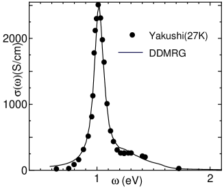
Figure 1: Optical conductivity spectra of K-TCNQ. The symbols show experimental result at 27 K in ref. yakushi, and the solid line is our DDMRG result for $N=40$.

Our best DDMRG result of $\sigma(\omega)$ and the experimental data by Yakushi et al. [31] are shown in Fig. 1. The DDMRG result is calculated for $U/t_{0}=5$, $V/t_{0}=1.7$, and $t_{0}=0.291{\rm eV}$, with the broadening parameter $\epsilon=0.16t_{0}$. As for the on-site Coulomb interaction $U$, our estimation is comparable to the values in the previous studies. [31, 32, 33] In addition, the relatively large $V$ is consistent with our previous conclusion that large $V$ is necessary to reproduce the sharp lowest peak and the broad higher-energy shoulder, [34] which are characteristic to K-TCNQ.

Then we determine $K_{\alpha}$ realizing $\delta=\delta_{\rm e}$ as the stable lattice configuration at half filling to be $K_{\alpha}=1.6/t_{0}$. Actually, the obtained stable lattice configuration at half filling with OBC is not completely uniformly dimerized. Besides a small boundary effect due to the OBC, there is a small difference between even and odd bonds: the number of even bonds is larger than that of odd bonds by one. Hence, we obtain the relaxed lattice configuration where the average of dimerization is equal to $\delta_{\rm e}$;

$$\frac{1}{N-1}\sum_{l=0}^{N-2}(-1)^{l}u_{l}/t_{0}=\delta_{e},$$ (10)

and then we confirm that $\sigma(\omega)$ for this stable configuration is almost identical to that for the uniformly dimerized configuration.

4 Polaronic States

Now, we discuss photogenerated polaronic states. In general, photoexcitation with energy corresponding to the charge transfer (CT) excitation generates two carriers. For 1D Mott insulators, these are known as a holon and a doublon. [35] In the experiment by H. Okamoto et al., the pump excitation with 1.55eV is considered to generate mobile holons and doublons. [17] These carriers move freely and are made separate within the time scale of $\hbar/t_{0}\sim 10^{-14}$ sec, which is much shorter than the experimental time resolution ($\sim 150$fs) [17] and the phonon dynamics. Hence, we consider that the lattice relaxation starts after the carriers are well-separated, suggesting the interaction effect between the carriers is negligible. Because of the particle-hole symmetry of this model, we consider the case where only one doublon exists on the system. We confirm that the case with a single holon shows the same results. As for the type of lattice relaxation, we consider the following cases: (case 1) $u$-relaxed and $v$-fixed, (case 2) $u$- and $v$-relaxed, and (case 3) $u$-fixed and $v$-relaxed, where $u(v)$-relaxed means that the intermolecular (intramolecular) distortion $u(v)$ is relaxed to the stable inhomogeneous configuration, and the $u(v)$-fixed denotes that the lattice configuration is fixed to the homogeneous one at half filling.

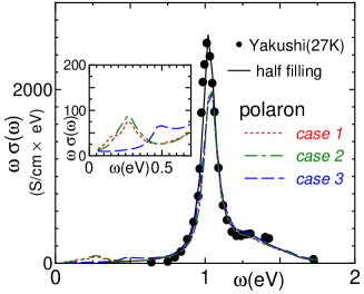
Figure 2: (Color online) Spectral functions for polaronic states where a single electron is introduced to $N=40$ systems. In cases 2 and 3, $K_{\beta}$ is set to $1.0/t_{0}$. The inset shows the magnified picture for the midgap region.

Figure 2 shows $\omega\sigma(\omega)$ of the polaron states for these three lattice configurations. The lowest-energy peak due to the open boundary condition is invisible in this and following figures. The results suggest that both of case 1 and case 2 well reproduce the midgap peak at 0.3 eV, although a small difference exists between them. The former shows a shoulder structure on the lower energy side of the main midgap peak. By contrast, case 2 seems to exhibit a single peak at 0.3eV. In case 3, there appears a midgap state above 0.5eV, being inconsistent with the experimental result. These observations suggest that the relaxation of $u$ is necessary to reproduce the experimental result.

The remaining problem is whether the relaxation of $v$ is necessary or not. In fact, we cannot reach the clear answer at present. The experimental resolution is not high enough to decide whether or not the low-energy shoulder is realized and to determine the plausible value of $K_{\beta}$. In the following, we only examine the origins of the characteristic peak structures of case 1 and case 2, which are the candidates for the polaron state of K-TCNQ.

5 Origins of Midgap States

5.1 Case 1

In Fig. 3, we plot $\omega\sigma(\omega)$ in case 1, and that of the unrelaxed lattice configuration (case 0), where $\bm{u}$ and $\bm{v}$ are the same as those at half filling. Further we show $\omega\sigma(\omega)$ for several intermediate lattice configurations between case 0 and case 1, defined as

$$\bm{u}(x)=\bm{u}({\rm case\ 0})+x[\bm{u}({\rm case\ 1})-\bm{u}({\rm case\ 0})],$$ (11)

where the degree of relaxation is denoted by $x$, and in Fig. 3, $x$ is shown in percentage.

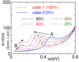
Figure 3: (Color online) Spectral functions for several lattice configurations (see the text).

The most intriguing is that a midgap peak, termed (A), appears at 0.5eV in case 0. Since no analog is present in noninteracting band insulators, this midgap peak is characteristic to the 1D dimerized Mott insulators. The peak (A) shifts toward lower energy as the lattice configuration approaches the completely $u$-relaxed one (100%). We also note that the other midgap peak, termed (B), appears in the lowest energy region for the slightly relaxed configuration ($x=20\%$). The peak (B) moves towards higher energy as the relaxation proceeds, and finally becomes a shoulder at $\bm{u}(100\%)$.

To clarify the origins of these midgap peaks, we calculate the optical conductivity spectra of unrelaxed systems with varying $U$ and $V$, which are shown in Fig. 4. We can see three different classes of midgap peaks. One is the metallic low-energy component in the lowest frequency region. This is the Drude “precursor” in the OBC case [36]. Another excitation is observed around $\omega\sim 3t_{0}$, which is well separated from the CT band for $U/t_{0}\geq 8$. This peak is caused by the intradimer CT excitation at the carrier site, while the carrier is mobile. [25] In ref. maeshima3, we argued that this CT excitation is a possible origin of the midgap peak in K-TCNQ. However, the present estimation of the model parameters for K-TCNQ ($U/t_{0}=5,V/t_{0}=1.7$) demonstrates that the corresponding peak is hidden by the CT excitations around $\omega\sim 4t_{0}$.

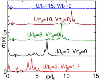
Figure 4: (Color online) Optical conductivity spectra for several sets of ($U,V$) with unrelaxed lattice configuration (case 0). The results are obtained with Lanczos diagonalization for $N=12$ systems with 7 electrons and the OBC imposed. The broadening parameter is set to $\epsilon=0.1t_{0}$. The filled circles show the singlet-triplet gap given by eq. (17)

Now we focus on the other class around $\omega/t_{0}=1-2$. For the parameter set corresponding to K-TCNQ, this peak is located at $\omega/t_{0}\sim 2$, which is identical to the midgap peak (A). Thus this midgap peak (A) can appear generally in 1D dimerized Mott insulators. It should be noted that its location is quite sensitive to $U$ and $V$; the excitation energy increases as $U$ decreases and as $V$ increases, implying that the midgap peak (A) is caused by spin excitations.

In fact, it can be shown that the excitation causing the peak (A) includes a singlet-triplet excitation. To show this, we use the analytical expression in the decoupled-dimer limit. [25] In the 0-th order approximation, the ground state of the system is represented by the direct product of the singlet-dimer states;

$$|\psi_{0}^{0}\rangle=|G\rangle_{0}\otimes|G\rangle_{1}\otimes\cdots\otimes|G\rangle_{N_{d}-1},$$ (12)

where $|G\rangle_{l},(l=0,\cdots,N_{d}-1)$ is the singlet-dimer state on the $l$-th dimer, and $N_{d}=N/2$. Then the one-electron-doped system is denoted by the linear combination of a direct product given by

$$|G\rangle_{0}\otimes|G\rangle_{1}\otimes\cdots\otimes|O^{3}_{\uparrow}\rangle_{n}\otimes\cdots\otimes|G\rangle_{N_{d}-1}.$$ (13)

Here, $|O^{3}_{\uparrow}\rangle_{n}$ has one more electron, and is defined as

$$|O^{3}_{\sigma}\rangle_{n}=\frac{1}{\sqrt{2}}(c^{\dagger}_{2n\bar{\sigma}}c^{\dagger}_{2n+1\sigma}c^{\dagger}_{2n\sigma}+c^{\dagger}_{2n+1\bar{\sigma}}c^{\dagger}_{2n+1\sigma}c^{\dagger}_{2n\sigma})|0\rangle,$$ (14)

with spin $\sigma$. Then we can construct a CT excitation via a interdimer CT process to obtain

$$|G\rangle_{0}\otimes\cdots\otimes|T\rangle_{n}\otimes|O^{3}_{\downarrow}\rangle_{n+1}\otimes\cdots\otimes|G\rangle_{N_{d}-1},$$ (15)

where

$$|T\rangle_{n}=c^{\dagger}_{2n\uparrow}c^{\dagger}_{2n+1\uparrow}|0\rangle.$$ (16)

A schematic picture of this excitation is given in Fig. 5 (a). Comparing eq. (13) and eq. (15), we find that the corresponding excitation energy $\Delta$ is equal to the singlet-triplet gap given by

$$\Delta=\frac{V-U}{2}+\sqrt{(U-V)^{2}/4+4t_{0}^{2}(1+\delta)^{2}}.$$ (17)

In Fig. 4, we plot $\Delta$ for each parameter set and find that $\Delta$ explains the excitation energy of the midgap peak (A).

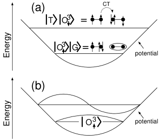
Figure 5: Schematic energy diagram for relevant midgap states (a) and (b) causing peaks (A) and (B), respectively.

The existence of two states, $|T\rangle_{n}$ and $|O^{3}_{\downarrow}\rangle_{m}$, is confirmed in the following analysis. If the state causing the peak (A) has these states, the doubly occupied site and the up spin must be separated ($n\neq m$). This is completely different from the states that include only $|O^{3}_{\uparrow}\rangle_{n}$, where the doubly occupied site and the up spin are located on the same dimer $n$. To demonstrate this spin-charge “separation”, we calculate the corresponding correction vector [37],

$$|\omega\rangle=A\frac{1}{({\cal H}-E_{0}-\omega)^{2}+\epsilon^{2}}J|\psi_{0}\rangle,$$ (18)

with normalization constant $A$. Figure 6 shows the charge and spin density profile of the correction vectors for a nearly completely relaxed configuration (80%). Here, we used the broadening parameter $\epsilon=0.16t_{0}$, whose result is found to be almost identical to that with $\epsilon=0.08t_{0}$ (not shown). We can see that the spin density of the state $|0.32{\rm eV}\rangle$ concentrates on the center of the lattice deformation and the charge density has a double peak beside the center, which shows that the spin and charge densities are separated as discussed above.

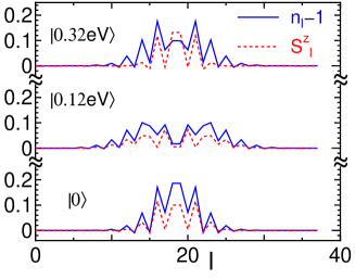
Figure 6: (Color online) Charge and spin distributions in several states for $x=80\%$ with $N=38$.

By contrast, the spin and charge densities of the state $|0.12{\rm eV}\rangle$ have similar distributions; both have double peaks and nodes at the center. Since the lowest state $|0\rangle$ has no node, the state causing the midgap peak (B) is the second lowest state made of the elementally excitation $|O^{3}_{\uparrow}\rangle$, as shown in Fig. 5 (b).

5.2 Case 2

Now, we turn our attention to case 2. Figure 7 shows the spectral function $\omega\sigma(\omega)$ in case 2 for several values of $K_{\beta}$. We can see that the shoulder structure (B) for $K_{\beta}t_{0}=\infty$ approaches the main peak (A) as $K_{\beta}$ decreases. Finally, these seem to merge into a single peak. This is because the excitation gap between the lowest polaron state and the second lowest state increases as the one-electron potential due to the intramolecular deformation $\bm{v}$ becomes deep, as shown in Fig. 8. By contrast, the intermolecular deformation $\bm{u}$ changes slightly, keeping the singlet-triplet gap $\Delta$ almost constant.

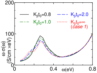
Figure 7: (Color online) Spectral functions in case 2.

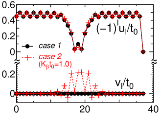
Figure 8: (Color online) Lattice configurations for case 1 and case 2 with $K_{\beta}t_{0}=1.0$ for $N=38$ systems.

6 Summary and Discussion

We have studied polaronic midgap states in the 1D extended Hubbard model with Peierls and Holstein types of electron-phonon couplings to clarify the origin of the midgap peak in K-TCNQ. Our main conclusion is that the relaxation of the intermolecular lattice distortion $\bm{u}$ is necessary to reproduce the observed midgap peak at 0.3 eV.

The midgap peak is numerically reproduced in the spectral function $\omega\sigma(\omega)$ for two polaronic lattice configurations. One has relaxed $\bm{u}$ and unrelaxed intramolecular vibration mode $\bm{v}$ (case 1), and the other has relaxed $\bm{u}$ and relaxed $\bm{v}$ (case 2). The former configuration is found to exhibit an additional shoulder structure on the lower energy side of the midgap peak. In this case, we have clarified the origins of the shoulder and the midgap peak.

The shoulder structure is caused by the excitation from the lowest bound state to the second-lowest state, both of which consist of the elementary excitation $|O^{3}_{\uparrow}\rangle$. This is similar to the polaron-based lower midgap peak of usual 1D band insulators, where the peak stems from the excitation from the lowest bound state to a higher state of introduced carriers (holes or electrons). [1, 38]

By contrast, the midgap peak is characteristic to 1D dimerized Mott insulators. The peak corresponds to the interdimer CT excitation from the state $|O^{3}_{\uparrow}\rangle$ to a superposition of the state $|O^{3}_{\downarrow}\rangle$ and the triplet dimer state $|T\rangle$. Its excitation energy is shown to exhibit spin-excitation-like $(U,V)$-dependence.

Our results provide some suggestions to the photoinduced inverse spin-Peierls “transition.” [16, 17, 18] First, the polaronic lattice relaxation proceeds within the experimental time resolution ($=$150fs). This implies that the phonon motion to generate the polaronic state is much faster than the observed coherent oscilation. [17] To discuss the speed of the phonon motion, we here evaluate the bare phonon frequency. The experimentally observed dimerization length ($\sim$ 0.165Å )[39] and the dimerization strength of the transfer integral ($\delta t_{0}=0.46\times 0.291$eV) lead to the e-ph coupling constant $\alpha\sim 0.81$ eV/Å. Then the unrenormalized elastic constant $K_{\alpha}$ is obtained to be 3.6 eV/Ų. These values for physical parameters give the bare phonon frequency $\omega=2\sqrt{K_{\alpha}/M_{\rm TCNQ}}\sim 2.6\times 10^{13}{\rm s}^{-1}$, where $M_{\rm TCNQ}\sim 3.4\times 10^{-25}{\rm kg}$ is the mass of a TCNQ molecule. Thus the speed of the bare phonon ($\sim$ sub ps) is found to be comparable to the experimental resolution time. It remains unresolved whether the bare phonon frequency determines the speed of the polaron formation or not.

Second, the photo-induced melting of the dimerization is explained by the “impurity (polaron) doping” picture [17], not by the mobile-carrier picture, [25] where the mobile photodoped carriers destroy the singlet dimerization of the dimerized phase. Third, one carrier can weaken the lattice dimerization roughly over 10 molecules as shown in Fig. 8. Assuming that interaction between doped carriers is negligible, we estimate that the dimerization order decreases linearly with respect to doping concentration at least up to 0.1 carrier per molecule. This is equivalent to 0.05 photon per molecule, which is equal to the photon density where the $\Delta R/R$ at 0.71 eV saturates [see Fig. 2(d) of ref. KTCNQ2].

Our estimation of the model parameters for K-TCNQ has demonstrated that K-TCNQ does not show the absorption peak caused by the conversion of photogenerated elementary excitations, which was proposed as the origin of the midgap peak. [25] This absorption for K-TCNQ is hidden by the CT excitation because the CT gap is nearly equal to the location of this absorption.

The existence of this conversion can be confirmed in other quasi-1D materials that have a larger CT gap. For example, an organic radical crystal, 1,3,5-trithia-2,4,6-triazapentalenyl (TTTA) is a candidate of these materials. [40] In ref. maeshima4, we have estimated model parameters for TTTA as $\delta=0.4$ and $U/t_{0}=10,V/t_{0}=1.7,t_{0}=0.235$ eV. Since this material has relatively large $U/t_{0}$, the absorption caused by the conversion can be well separated from the CT band.

References

- [1] A. J. Heeger, S. Kivelson, J. R. Schrieffer and W. P. Su: Rev. Mod. Phys. 60 (1988) 781.
- [2] H. Okamoto and M. Yamashita: Bull. Chem. Soc. Jpn. 71 (1998) 2023.
- [3] K. Nasu: Rep. Prog. Phys. 67 (2004) 1607.
- [4] K. Yonemitsu and K. Nasu: J. Phys. Soc. Jpn. 75 (2006) 011008.
- [5] G. Yu, C. H. Lee, A. J. Heeger, N. Herron, and E. M. McCarron: Phys. Rev. Lett. 67 (1991) 2581.
- [6] M. Fiebig, K. Miyano, Y. Tomioka, and Y. Tokura: Science 280 (1998) 1925.
- [7] A. Cavalleri, Cs. Tóth, C. W. Siders, J. A. Squier, F. Ráksi, P. Forget, and J. C. Kieffer: Phys. Rev. Lett. 87 (2001) 237401.
- [8] L. Perfetti, P. A. Loukakos, M. Lisowski, U. Bovensiepen, H. Berger, S. Biermann, P. S. Cornaglia, A. Georges, and M. Wolf: Phys. Rev. Lett. 97 (2006) 067402.
- [9] S. Koshihara, Y. Tokura, T. Mitani, G. Saito, and T. Koda: Phys. Rev. B 42 (1990) 6853.
- [10] E. Collet, M.-H. Lemee-Cailleau, M. Buron-Le Cointe, H. Cailleau, M. Wulff, T. Luty, S. Koshihara, M. Meyer, L. Toupet, P. Rabiller, and S. Techert: Science 300 (2003) 612.
- [11] S. Koshihara, Y. Tokura, K. Takede, and T. Koda: Phys. Rev. Lett. 68 (1992) 1148.
- [12] S. Iwai, M. Ono, A. Maeda, H. Matsuzaki, H. Kishida, H. Okamoto, and Y. Tokura: Phys. Rev. Lett. 91 (2003) 057401.
- [13] H. Matsuzaki, T. Matsuoka, H. Kishida, K. Takizawa, H. Miyasaka, K. Sugiura, M. Yamashita, and H. Okamoto: Phys. Rev. Lett. 90 (2003) 046401.
- [14] M. Chollet, L. Guerin, N. Uchida, S. Fukaya, H. Shimoda, T. Ishikawa, K. Matsuda, T. Hasegawa, A. Ota, H. Yamochi, G. Saito, R. Tazaki, S. Adachi, and S. Koshihara: Science 307 (2005) 86.
- [15] N. Tajima, J. Fujisawa, N. Naka, T. Ishihara, R. Kato, Y. Nishio, and K. Kajita: J. Phys. Soc. Jpn. 74 (2005) 511.
- [16] S. Koshihara, Y. Tokura, Y. Iwasa, and T. Koda: Phys. Rev. B 44 (1991) 431.
- [17] H. Okamoto, K. Ikegami, T. Wakabayashi, Y. Ishige, J. Togo, H. Kishida, and H. Matsuzaki: Phys. Rev. Lett. 96 (2006) 037405.
- [18] K. Ikegami, K. Ono, J. Togo, T. Wakabayashi, Y. Ishige, H. Matsuzaki, H. Kishida, and H. Okamoto: Phys. Rev. B 76 (2007) 085106.
- [19] H. Matsuzaki, W. Fujita, K. Awaga, and H. Okamoto: Phys. Rev. Lett. 91 (2003) 017403.
- [20] J. Takeda, M. Imae, O. Hanado, S. Kurita, M. Furuya, K. Ohno, and T. Kodama: Chem. Phys. Lett. 378 (2003) 456.
- [21] H. Matsueda and S. Ishihara: J. Phys. Soc. Jpn. 76 (2007) 083703.
- [22] J. G. Vegter, T. Hibma, and J. Kommandeur: Chem. Phys. Lett. 3 (1969) 427.
- [23] N. Sakai, I. Shirotani, and S. Minomura: Bull. Chem. Soc. Jpn. 45 (1972) 3321.
- [24] H. Terauchi: Phys. Rev. B 17 (1978) 2446.
- [25] N. Maeshima and K. Yonemitsu: Phys. Rev. B 74 (2006) 155105.
- [26] S. R. White: Phys. Rev. Lett. 66 (1992) 2863.
- [27] K. A. Hallberg: Phys. Rev. B 52 (1995) R9827.
- [28] T. D. Kühner and S. R. White: Phys. Rev. B 60 (1999) 335.
- [29] E. Jeckelmann: Phys. Rev. B 66 (2002) 045114.
- [30] The formula for the optical conductivity is given, for example, by B. S. Shastry and B. Sutherland: Phys. Rev. Lett. 65 (1990) 243.
- [31] K. Yakushi, T. Kusaka, and H. Kuroda: Chem. Phys. Lett. 68 (1979) 139.
- [32] M. Meneghetti: Phys. Rev. B 44 (1991) 8554.
- [33] F. B. Gallagher and S. Mazumdar: Phys. Rev. B 56 (1997) 15025.
- [34] N. Maeshima and K. Yonemitsu: J. Phys. Soc. Jpn. 76 (2007) 074713.
- [35] Y. Mizuno, K. Tsutsui, T. Tohyama, and S. Maekawa: Phys. Rev. B 62 (2000) R4769.
- [36] R. M. Fye, M. J. Martins, D. J. Scalapino, J. Wagner, and W. Hanke: Phys. Rev. B 44 (1991) 6909.
- [37] K. Iwano: Phys. Rev. Lett 97 (2006) 226404.
- [38] Y. Tagawa and N. Suzuki: J. Phys. Soc. Jpn. 59 (1990) 4074.
- [39] M. Konno, T. Ishii, and Y. Saito: Acta Cryst. B33, (1977) 763.
- [40] W. Fujita and K. Awaga: Science 286 (1999) 261.