Shell States of Neutron Rich Matter

Abstract

The equation of state (EOS) for nuclear and neutron rich matter is investigated in a Relativistic Mean Field (RMF) model. New shell states are found that minimize the free energy per baryon, calculated in a spherical Wigner-Seitz (WS) approximation, over a significant range of baryon densities. These shell states, that have both inside and outside surfaces, minimize the Coulomb energy of large proton number configurations at the expense of a larger surface energy. This is related to a possible depression in the central density of super heavy nuclei. As the baryon density increases, we find the system changes from normal nuclei, to shell states, and then to uniform matter.

I Introduction

The equation of state (EOS) for dense nuclear matter plays an important role in understanding the structure of neutron stars and for simulations of core collapse supernovae. Neutron stars probe the zero temperature EOS while supernovae involve the EOS at temperatures up to tens of MeV. Below the neutron drip density, $\approx 2\times 10^{11}$ g/cm³ where free neutrons appear, knowledge of the EOS can be extrapolated from the properties of laboratory atomic nuclei. In contrast, current terrestrial experiments only constrain the EOS above neutron drip density with rather big uncertainties. Recently, there have been efforts from heavy ion collision experiments heavyions , X-ray observations of isolated neutron stars x-rays , and theoretical calculations to understand the EOS beyond the neutron-drip point.

There have been many calculations of nonuniform matter at sub-nuclear density, below $3\times 10^{14}$ g/cm³. Negele and Vautherin, using a Skyrme Hartree-Fock calculation with two-body potentials Negele , obtained the ground state within the spherical Wigner-Seitz (WS) approximation. In this approximation, the unit cell of a crystal lattice is modeled as a sphere. They found, as the system became more neutron rich and the density increased, neutrons escaped and the system approached a uniform state near nuclear density. Since then there have been many investigations more with more sophisticated interactions and more complicated lattice configurations, such as cylinders or plates. These non-spherical ’pasta’ phases, which seem to appear within a significant range of sub-nuclear densities are relevant for the structure of neutron star crusts crust1 ; crust2 and the dynamics of supernovae sn .

For hot nuclear matter, assuming that the spherical WS cell still remains a good approximation to the realistic lattice structure, people have studied the EOS with different models. Using a phenomenological compressible liquid-drop model, Lattimer and Swesty LSeos produced an equation of state for hot dense matter that has been widely used in supernova simulations. Later, H. Shen et. al. HSeos constructed an equation of state based on Thomas-Fermi and variational approximations to a relativistic mean field energy functional. Neither method takes into account the shell structure of finite nuclei or explores the full range of density distributions possible even in the spherical WS approximation.

In recent years, relativistic mean field models (RMF) have provided a consistent description for the ground state properties of finite nuclei, both along and far away from the valley of beta stability HS1 ; HS2 ; SW ; Rein ; Ring . These models incorporate the spin-orbit splitting naturally and the relativistic formalism provides a framework to extrapolate the properties of non-uniform and uniform nuclear matter to high densities. Furthermore there is a close relation between phenomenalogical RMF models, that simply fit parameters to properties of finite nuclei, and more systematic effective field theory approaches that enumerate all of the possible interactions that are allowed by symmetries.

In this work, we develop a RMF code to explore the equation of state for non-uniform and uniform nuclear matter at finite temperatures with a range of proton fractions and wide range of baryon densities. For non-uniform nuclear matter, we use the spherical WS approximation to find the stable state for a charge neutral system of neutrons, protons and electrons. In this paper, we will focus on the matter at a low temperature T =1 MeV. It is easier for us to find the ground state at T = 0 by extrapolating the theory at a low temperature T $\neq$ 0 to T = 0, because the occupations of nucleon levels vary more smoothly at finite temperature. In the future we will also study the EOS at higher temperatures.

For nonuniform matter we find new shell states which minimize the free energy per baryon over a significant density range. Shell states have inside and outside surfaces and they can minimize the Coulomb energy of high $Z$ (large proton number) configurations at the expense of a larger surface energy. These shell states may be related to the appearance of a central depression in the density of super heavy nuclei heavy because of their large coulomb energies. The appearance of shell states may significantly change transport properties such as the shear viscosity and shear modulus of neutron rich matter.

We compare the transition density, that we find in nonuniform RMF calculations, to that predicted from a stability analysis of uniform nuclear matter. We start from uniform matter in equilibrium, and then find the critical density when the longitudinal collective mode, that describes density oscillations, becomes unstable.

The paper is organized as follows. First in Section II, we give a brief description of the RMF theory at finite temperature and explain the WS approximation for non-uniform matter. Next, Section II.2 presents the collective mode analysis for uniform matter in both the Vlasov formalism and using the RPA approximation. In Section III, we present results for the EOS of nonuniform matter. Finally in Section IV, we summarize our results and comment on future work.

II Formalism

The RMF theory and its applications have been reviewed in a number of places, see for example Refs. SW ; Rein ; Ring . The basic ansatz of the RMF theory is a Lagrangian density where nucleons interact via the exchange of sigma- ($\sigma$), omega- ($\omega$), and rho- ($\rho$) mesons, and also photons ($A$).

$${\cal L} = \overline{\psi}[i{\gamma^{\mu}}{\partial_{\mu}}-m-{g_{\sigma}}\sigma-g_{\omega}\gamma^{\mu}\omega_{\mu}$$ (1)

$$-\ g_{\rho}\gamma^{\mu}\vec{{\bf\tau}}\cdot\vec{\mbox{\boldmath$\rho$}}_{\mu}-e\gamma^{\mu}\frac{1+\tau_{3}}{2}A_{\mu}]\psi$$

$$+\ \frac{1}{2}\partial^{\mu}\sigma\partial_{\mu}\sigma-\frac{1}{2}m_{\sigma}^{2}\sigma^{2}-\frac{1}{3}g_{2}\sigma^{3}\ -\ \frac{1}{4}g_{3}\sigma^{4}$$

$$-\ \frac{1}{4}\omega^{\mu\nu}\omega_{\mu\nu}+\frac{1}{2}m_{\omega}^{2}\omega^{\mu}\omega_{\mu}+\frac{1}{4}c_{3}\left(\omega^{\mu}\omega_{\mu}\right)^{2}$$

$$-\ \frac{1}{4}\vec{\mbox{\boldmath$\rho$}}^{\mu\nu}\cdot\vec{\mbox{\boldmath$\rho$}}_{\mu\nu}+\frac{1}{2}m_{\rho}^{2}\vec{\mbox{\boldmath$\rho$}}^{\mu}\cdot\vec{\mbox{\boldmath$\rho$}}_{\mu}-\ \frac{1}{4}A^{\mu\nu}A_{\mu\nu}$$

Here the field tensors of the vector mesons and the electromagnetic field take the following forms:

$$\omega^{\mu\nu} = \partial^{\mu}\omega^{\nu}-\partial^{\nu}\omega^{\mu},$$

$$A^{\mu\nu} = \partial^{\mu}A^{\nu}-\partial^{\nu}A^{\mu},$$

$$\vec{\mbox{\boldmath$\rho$}}^{\mu\nu} = \partial^{\mu}\vec{\mbox{\boldmath$\rho$}}^{\nu}-\partial^{\nu}\vec{\mbox{\boldmath$\rho$}}^{\mu}-g_{\rho}\vec{\mbox{\boldmath$\rho$}}^{\mu}\times\vec{\mbox{\boldmath$\rho$}}^{\nu}\,.$$ (2)

In charge neutral nuclear matter composed of neutrons, $n$, protons, $p$, and electrons, $e$, there are equal numbers of electrons and protons. Electrons can be treated as a uniform Fermi gas at high densities. They contribute to the Coulomb energy of the $npe$ matter and serve as one source of the Coulomb potential.

The variational principle leads to the following equations of motion

$$[\mathbf{\sl{\alpha}}\cdot\mathbf{\sl{p}}\ +\ V(\mathbf{r})\ +\ \sl{\beta}(m\ +\ S(\mathbf{r}))]\psi_{i}\ =\ \varepsilon_{i}\psi_{i}$$ (3)

for the nucleon spinors, where

$$\left\{\begin{array}[]{l}V(\mathbf{r})=\ \beta\{g_{\omega}\hbox to0.0pt{/\hss}{\omega}_{\mu}\ +\ {g_{\rho}}\vec{\tau}\cdot\vec{\hbox to0.0pt{/\hss}\rho_{\mu}}\ +\ e\frac{(1\ +\ \tau_{3})}{2}\ \hbox to0.0pt{/\hss}A_{\mu}\}\\ S(\mathbf{r})=\ g_{\sigma}\sigma\end{array}\right.$$ (6)

and

$$\left\{\begin{array}[]{l}(m_{\sigma}^{2}\ -\ \nabla^{2})\ \sigma=\ -g_{\sigma}\rho_{s}-\ g_{2}\sigma^{2}\ -\ g_{3}\sigma^{3}\\ (m_{\omega}^{2}\ -\ \nabla^{2})\omega^{\mu}=\ g_{\omega}j^{\mu}-c_{3}\omega^{\mu}(\omega^{\nu}\omega_{\nu})\\ (m_{\rho}^{2}\ -\ \nabla^{2})\vec{\rho}^{\mu}=\ {g_{\rho}}\vec{j}^{\mu}\\ \hskip 25.00003pt-\ {\nabla}^{2}A^{\mu}=\ e(j^{\mu}_{p}-j^{\mu}_{e})\end{array}\right.$$ (11)

for the mesons and photons, where the electrons are included as a source of Coulomb potential. The nucleon spinors provide the relevant source terms:

$$\left\{\begin{array}[]{l}\rho_{s}=\ \sum_{i}\overline{\psi}_{i}\psi_{i}n_{i}\\ j^{\mu}=\ \sum_{i}\overline{\psi}_{i}\gamma^{\mu}\psi_{i}n_{i}\\ \vec{j}^{\mu}=\ \sum_{i}\overline{\psi}_{i}\gamma^{\mu}\vec{\tau}\psi_{i}n_{i}\\ j^{\mu}_{p}=\ \sum_{i}\overline{\psi}_{i}\gamma^{\mu}\frac{1+\tau_{3}}{2}\psi_{i}n_{i}.\end{array}\right.$$ (15)

At zero temperature, the summations run over the valence nucleons only, since $n_{i}=\Theta(\varepsilon_{F}-\varepsilon_{i})$ where $\varepsilon_{F}$ is the Fermi energy of the nucleons. At finite temperature, Fermi-Dirac statistics prescribes the occupations of protons and neutrons as follows:

$$n_{i}\ =\ \frac{1}{e^{\beta(\varepsilon_{i}-\mu)}+1},$$ (16)

where $\mu$ is the chemical potential for neutron (proton). In practice, we include all levels with $n_{i}>10^{-8}$.

Since the systems under consideration have temperatures of, at most, tens of MeV, we neglect the contribution of negative energy states, i.e., the so-called no sea approximation. In a spherical nucleus, there are no currents in the nucleus and the spatial vector components of $\omega_{\mu}$, $\vec{\rho}_{\mu}$ and $A_{\mu}$ vanish. One is left with the timelike components. Charge conservation guarantees that only the 3-component of the isovector $\rho_{0,3}$ survives. The above non-linear equations are solved by iteration within the context of the mean field approximation whereby the meson field operators are replaced by their expectation values.

II.1 Nonuniform Matter with Wigner-Seitz approximation

The spherical Wigner-Seitz (WS) approximation is used to describe non-uniform matter. In general the unit cell of a crystal lattice is a complex close-packed polyhedron. This is approximated by a spherical cell of the same volume. We apply boundary conditions on the wave functions at the edge of WS unit cell. To achieve a uniform density distribution for a free neutron gas, we require that at the cell radius, all wave functions of even parity vanish, and the radial derivative of odd parity wave functions also vanishes Negele .

In the WS approximation, the lattice Coulomb energy consists of contributions from neighboring unit cells. This correction to the WS Coulomb energy is important for determining the stable configuration of WS cells and the transition density to uniform matter, especially when the system has a large proton fraction. We include the exact Coulomb energy in calculating the free energy of WS cell of radius $R_{c}$. Following the treatment in Ref. Kittel ; Oyamatsu , we calculate the Coulomb energy per unit cell as,

$$W_{c}=\frac{1}{2}\sum_{\vec{G}}^{\prime}\frac{I_{hkl}^{2}}{a^{3}\vec{G}^{2}},$$ (17)

where $a$ is lattice constant defined by $a^{3}=V_{cell}=\frac{4\pi}{3}R_{c}^{3}$, and

$$\vec{G}=h\vec{A}+k\vec{B}+l\vec{C}.$$ (18)

Here $h,k$, and $l$ are integers, and $\vec{A}$, $\vec{B}$, and $\vec{C}$ are the primitive transformation vectors of the reciprocal lattice. The prime on the sum means that the point $\vec{G}$ = 0 is excluded. The form factor $I_{hkl}$ is given by

$$I_{hkl}=\int_{cell}\rho_{p}(\vec{r})e^{-i\vec{G}\cdot\vec{r}}d\vec{r}.$$ (19)

Oyamatsu et al. Oyamatsu assumed a uniform proton density inside the nucleus and found that the stable configuration is a Body-Centered Cubic (BCC) lattice. Using realistic proton density distribution, we also find that a BCC lattice gives the lowest Coulomb energy. In principle, one needs to worry about the screening of Coulomb interactions by electrons. It turns out that screening contributions to the Coulomb energy are very small crust1 and we will neglect them in our calculations.

With the approximations specified above, it is convenient to perform a self-consistent relativistic mean field Hartree calculation for nuclear wave functions inside a WS cell of radius $R_{c}$, for given average baryon density $\rho_{B}$, proton fraction $Y_{p}$ and temperature $T$. The nucleon number inside the WS cell is therefore $A=4\pi R_{c}^{3}\rho_{B}/3$ and proton number $Z=Y_{p}A$. The total energy of the WS cell, including the exact lattice Coulomb energy, is obtained as follows,

$$E_{b} = E_{nucleon}+E_{\sigma}+E_{\rho}+E_{\omega}+W_{c}-mA$$ (20)

$$= \sum_{i}\epsilon_{i}n_{i}-\ e\int\rho_{p}A_{0}(r)d^{3}r\ -\ \frac{1}{2}\int d^{3}r\{g_{\sigma}\sigma\rho_{s}(r)\$$ (23)

$$+\ \frac{1}{3}g_{2}\sigma^{3}\ +\ \frac{1}{2}g_{3}\sigma^{4}\}\ -\ \frac{1}{2}\int d^{3}rg_{\rho}\rho_{0,3}j_{0,3}(r)\$$

$$-\ \frac{1}{2}\int d^{3}r\{g_{\omega}\omega_{0}\ j_{0}(r)-\ \frac{1}{2}c_{3}\omega_{0}^{4}\}+\ W_{c}-mA.$$

The nucleon contribution to the entropy is given by the usual formula,

$$S_{b}=-k_{B}\sum_{i}\left[n_{i}\mathrm{ln}(n_{i})\ +(1-n_{i})\mathrm{ln}(1-n_{i})\right],$$ (25)

where $n_{i}$ is given in Eq. (16). With Eqs. (20) and (25), it is easy to obtain the nucleon contribution to the free energy per baryon $f_{b}$,

$$f_{b}=F_{b}/A=(E_{b}\ -\ TS_{b})/A.$$ (26)

We also include the contribution of free electrons. Explicit formulas for the electron contribution to the free energy per baryon $f_{e}$, and entropy $S_{e}$ of the electron gas are presented in Ref. LSeos . Finally, the complete free energy per baryon is

$$f=f_{b}+f_{e}.$$ (27)

II.2 Stability analysis

II.2.1 Semiclassical collective modes analysis

The unstable collective modes of uniform $npe$ matter at finite temperature can be investigated in the RMF by using a Vlasov formalism Brito06 . Here we give a short summary to make this paper more self-contained.

The distributions of particles (antiparticles) denoted as + (-), at position $\mathbf{r}$, time $t$, and momentum $\mathbf{k}$ ($\mathbf{-k}$) are described via the phase space distribution functions as following:

$$f(\mathbf{r},\mathbf{k},t)_{\pm}\ =\ \mathrm{diag}(f_{p\pm},f_{n\pm},f_{e\pm}).$$ (28)

The time evolution of distribution functions are determined by the Vlasov equation:

$$\frac{\partial f_{i\pm}}{\partial t}\ +\ \{f_{i\pm},h_{i\pm}\}=0,i=p,n,e,$$ (29)

where { , } denotes the Poisson brackets. $h_{i\pm}$ is the one body Hamiltonian, which can be derived from Eq. (1) for neutrons and protons. For electrons, $h$ is the normal QED Hamiltonian. Small deviations $\delta f_{\pm}$ of the distribution functions around the equilibrium state can be calculated with generating functions

$$S(\mathbf{r},\mathbf{k},t)_{\pm}\ =\ \mathrm{diag}(S_{p\pm},S_{n\pm},S_{e\pm}),$$ (30)

such that

$$\delta f_{\pm}\ =\ \{S_{\pm},f_{0\pm}\}\ =\ \{S_{\pm},k^{2}\}\frac{df_{0\pm}}{dk^{2}},$$ (31)

where $f_{0\pm}$ are equilibrium distribution functions. In terms of the generating functions, one can obtain linearized Vlasov equation for $\delta f_{\pm}$. From the equations of motion for meson and photon fields, one can also get the linearized equations for the oscillation fields.

The dominant collective modes at low temperatures are the longitudinal modes (with momentum $\mathbf{p}$ and frequency $\Omega$), which can be described by the ansatz

$$\left(\begin{array}[]{c}S_{j\pm}(\mathbf{r},\mathbf{k},t)\\ \delta\sigma\\ \delta B^{\mu}\end{array}\right)\ =\ \left(\begin{array}[]{c}S^{j}_{\Omega\pm}(k,\cos\theta)\\ \delta\sigma_{\Omega}\\ \delta B^{\mu}_{\Omega}\end{array}\right)\ e^{i(\Omega t-\mathbf{p}\cdot\mathbf{r})},$$ (32)

where $j=p,n,e$, $B^{\mu}=\omega^{\mu},\rho^{\mu},A^{\mu}$ represents the vector fields and photon fields. $\theta$ is the angle between $\mathbf{p}$ and $\mathbf{k}$. After transforming the unknown variables to the density oscillations of $p,n,e$, we can obtain the following matrix equation for the eigenmodes

$$D(\Omega)\left(\begin{array}[]{c}\delta\rho^{S}_{\Omega p}\\ \delta\rho^{S}_{\Omega n}\\ \delta\rho_{\Omega p}\\ \delta\rho_{\Omega n}\\ \delta\rho_{\Omega e}\end{array}\right)\ =\ 0,$$ (33)

where $\delta\rho^{S}_{\Omega p}$ and $\delta\rho^{S}_{\Omega n}$ are the amplitudes of the oscillating scalar densities of protons and neutrons, respectively, and $\delta\rho_{\Omega p}$, $\delta\rho_{\Omega n}$, and $\delta\rho_{\Omega e}$ are the amplitudes of the oscillating proton, neutron, and electron densities. The entries of the matrix $D(\Omega)$ are given in Ref. Brito06 .

The spectrum of collective modes, or the dispersion relation $\Omega=\Omega(p)$, is determined by the eigen condition $D(\Omega)=0$. The instability of collective modes can be deduced directly from the static limit of the dispersion relation, i.e., if $D(\Omega=0)\leq 0$, the collective modes will be unstable and exponentially growing. This indicates a phase transition to non-uniform matter.

II.2.2 RPA at finite temperature

We now perform a second very similar stability analysis using the random phase approximation (RPA). This provides an independent check of the Vlasov approach. A detailed account of the finite temperature RPA method for Quantum Hadrodynamics can be found in Ref. ftRPA . Again we present some information to demonstrate the idea. The finite temperature Feynman rules yield the $(s,s^{\prime})$ thermal component of the causal polarization insertion for particle species $i$ $(i=n,p,e)$ as

$$\underline{\Pi}^{C(s,s^{\prime})}_{\mu\nu(i)}\ = \ -i\int\frac{d^{4}k}{(2\pi)^{4}}(-1)^{(s+s^{\prime})}\mathrm{Tr}[G_{H(i)}^{(s,s^{\prime})}(k)J_{\mu}(i)$$ (35)

$$\times G_{H(i)}^{(s^{\prime},s)}(k+q)J_{\nu}(i)],$$

where $G_{H(i)}^{(s,s^{\prime})}$ is the $(s,s^{\prime})$ thermal component of Hartree propagators of species $i$. For $\gamma$(photon), $\omega$, and $\rho$ meson, $J_{\mu}=\gamma_{\mu}$, and the polarization is a tensor $\underline{\Pi}_{\mu\nu}$. For the $\sigma$ meson $J_{\mu}=1$, and the polarization is a scalar $\underline{\Pi}_{s}$. If $J_{\mu}=\gamma_{\mu}$ and $J_{\nu}=1$ (or vice versa), the polarization is mixed $\underline{\Pi}_{M\mu}$.

At finite temperature, Dyson’s equation for the proper longitudinal causal polarization is a matrix with particle, Lorentz, and thermal indices. It can be written as

$$\underline{\widetilde{\Pi}}^{c}_{L}\ =\ \underline{\Pi}^{c}_{L}\ +\ \underline{\widetilde{\Pi}}^{c}_{L}\underline{D}^{0}\underline{\Pi}^{c}_{L},$$ (36)

where $\underline{D}^{0}$ is the lowest order thermal matrix for the meson/photon propagator. For example, for scalar meson propagator is

$$\underline{D}^{0}(k)=\underline{M}_{b}\left(\begin{array}[]{cc}\Delta_{F}(k)&0\\ 0&-\Delta_{F}^{+}(k)\\ \end{array}\right)\underline{M}_{b},$$ (37)

where $\Delta_{F}(k)$ is the normal Feynman propagator and $\underline{M}_{b}$ is the thermal matrix defined as

$$\underline{M}_{b}=\left(\begin{array}[]{cc}\cosh\theta&-\sinh\theta\\ \sinh\theta&\cosh\theta\\ \end{array}\right).$$ (40)

The angle $\theta$ is given by $\sinh\theta=[\exp\beta|k_{0}|-1]^{-1/2}$, with inverse temperature $\beta$. The thermal vector meson propagator has the same structure.

At finite temperature we can also define

$$\underline{\varepsilon}_{L}=\ 1\ -\ \underline{D}^{0}\underline{\Pi}^{c}_{L},$$ (41)

which allows us to derive the dielectric function by the real part of its (11) component,

$$\varepsilon_{L}(q_{\mu})\ =\ \mathrm{det}\mathrm{Re}(\underline{\varepsilon}_{L}(q_{\mu})^{11}) = \ \mathrm{det}\{1-\Delta_{F}\mathrm{Re}\Pi_{L}^{c(11)}\},$$ (42)

where we have used $\mathrm{Re}\Pi_{L}^{c(11)}=\mathrm{Re}\Pi_{L}^{c}$. The poles of the dielectric function define the collective mode excitations of uniform matter. The dielectric function in the static limit determines the stability of the modes. When

$$\varepsilon_{L}(q_{0}=0,q)\leq 0,$$ (44)

the system is unstable against small amplitude longitudinal collective oscillations (density fluctuations). This indicates a phase transition to non-uniform matter.

The above equation is for one particle species and one boson interaction. This can be generalized to several particle species with multiple interactions. For a system consisting of neutrons, protons, and electrons, the interaction matrix and polarization matrix are given as

$$D_{L}^{0}\ = \ \left(\begin{array}[]{cccc}D_{g}^{0}&0&-D_{g}^{0}&0\\ 0&-D_{s}^{0}&0&0\\ -D_{g}^{0}&0&D_{g}^{0}+D_{v}^{0}+D_{\rho}^{0}&D_{v}^{0}-D_{\rho}^{0}\\ 0&0&D_{v}^{0}-D_{\rho}^{0}&D_{v}^{0}+D_{\rho}^{0}\\ \end{array}\right),$$ (49)

$$\mathrm{Re}\Pi_{L}^{c(11)}\ = \ \left(\begin{array}[]{cccc}\Pi_{00}^{e(11)}&0&0&0\\ 0&\Pi_{s}^{n(11)}+\Pi_{s}^{p(11)}&\Pi_{M}^{p(11)}&\Pi_{M}^{n(11)}\\ 0&\Pi_{M}^{p(11)}&\Pi_{00}^{p(11)}&0\\ 0&\Pi_{M}^{n(11)}&0&\Pi_{00}^{n(11)}\\ \end{array}\right).$$ (55)

The explicit formula for these polarizations are listed in Ref. ftRPA . For the Lagrangian in Eq. (1), the corresponding meson propagators are

$$D_{g}^{0}\ = \ \frac{4\pi\alpha}{q^{2}},$$ (57)

$$D_{s}^{0}\ = \ \frac{g_{\sigma}^{2}}{q^{2}+m_{\sigma}^{*2}},$$ (58)

$$D_{v}^{0}\ = \ \frac{g_{\omega}^{2}}{q^{2}+m_{\omega}^{*2}},$$ (59)

$$D_{\rho}^{0}\ = \ \frac{g_{\rho}^{2}}{q^{2}+m_{\rho}^{2}},$$ (60)

where the effective masses are defined as

$$m_{\sigma}^{*2}\ = \ m_{\sigma}^{2}\ +\ 2g_{2}\sigma\ +\ 3g_{3}\sigma^{2},$$ (61)

$$m_{\omega}^{*2}\ = \ m_{\omega}^{2}+3c_{3}\omega_{0}^{2}.$$ (62)

III Results

In this work we use the NL3 effective interaction NL3 that has been successful in reproducing ground state properties of stable nuclei and the saturation properties of symmetric nuclear matter. The values of parameters for the NL3 effective interaction are listed in Table 1. In this section, we present results in the spherical WS approximation for non-uniform matter at a temperature of $T=1$ MeV.

To determine the minimum free energy per baryon $f$ in Eq. (27) at a specified baryon density $\rho_{B}$, one must search over the cell radius $R_{c}$. When $R_{c}$ is large and $\rho_{B}$ is beyond the neutron drip density, one will need to take into account a large number of levels, since the nucleon number is $A=4\pi R_{c}^{3}\rho_{B}/3$. The fact that the matter is at finite temperature will require one to consider even more levels. For example, when $\rho_{B}$ = 0.080 fm^-3, $Y_{p}$ = 0.4, and $R_{c}$ = 23.5 fm, there are 4892 nucleons inside one WS cell and one needs to include 427 (419) neutron (proton) levels. It is hard to achieve self-consistency for the mean fields with a large number of levels. To ensure the convergence of the self-consistent iterations for the mean fields, it is important to have a good initial guess for the mean field potentials. Here our strategy is to employ the convergent potentials for a nucleus with a smaller $R_{c}$ as the starting guess for a nucleus with a slightly larger $R_{c}$. In this way, new shell states with large cell radii are found. These can minimize the free energy over a significant density range.

Table 1: NL3 effective interaction. The nucleon masses are $M$ = 939 MeV for both protons and neutrons and $c_{3}=0$.

$g_{\sigma}$	$g_{\omega}$	$g_{\rho}$	$g_{2}$	$g_{3}$	$m_{\sigma}$	$m_{\omega}$	$m_{\rho}$
			(fm-1)		(MeV)	(MeV)	(MeV)
10.217	12.868	4.474	-10.431	-28.885	508.194	782.5	763

We show in Fig. 1 an example of how shell states were found. Here the free energy per baryon versus WS cell radius is displayed for baryon densities of 0.040, 0.049, 0.080, and 0.090 fm^-3 when $Y_{p}$ =0.4. For each baryon density, there are two minima of free energy per baryon at different WS radii, denoted as open circles. The neutron and proton density distributions of the WS cells with these two radii are shown in Fig. 2. The first minimum at smaller WS cell radius corresponds to a nucleus with a normal density distribution. The second minimum at larger WS cell radius corresponds to a shell shaped density distribution. Here the nucleus has both outside and inside surfaces and the neutron and proton densities are only non-vanishing at intermediate $r$. We call the first minimum a nucleus state and the second minimum a shell state. For the shell state, the sum of neutron and proton densities (at intermediate $r$) is close to the saturation density of nuclear matter $\sim$ 0.15 fm^-3, as one expects from nuclear saturation.

At $\rho_{B}$ = 0.049 fm^-3, the two minima of free energy per baryon become degenerate, as shown in upper right panel of Fig. 1. Below 0.049 fm^-3, the first minimum with smaller cell radius corresponding to a normal nucleus is the absolute minimum and therefore the equilibrium state (e.g., panel a of Fig. 1). On the other hand, above 0.049 fm^-3, the second minimum corresponding to a shell state is the true equilibrium state (e.g., panels c and d of Fig. 1). Therefore 0.049 fm^-3 is the critical baryon density when the density distribution inside the WS cell changes from a normal nucleus to a shell state. In the lower right panel of Fig. 2, we also show the uniform neutron and proton density distributions by dotted lines when $\rho_{B}$ = 0.090 fm^-3. As will be shown later, 0.090 fm^-3 is the transition density from a shell state to uniform matter.

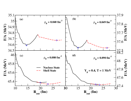
Figure 1: (Color online) Free energy per baryon versus Wigner-Seitz cell radius $R_{c}$ for baryon densities of $\rho_{B}$ = 0.040 (a), 0.049 (b), 0.080 (c), and 0.090 fm^-3 (d). The proton fraction is $Y_{p}=0.4$ and the temperature is $T$ = 1 MeV. The two circles denote minima for the nucleus (small $R_{c}$) and shell states (larger $R_{c}$).

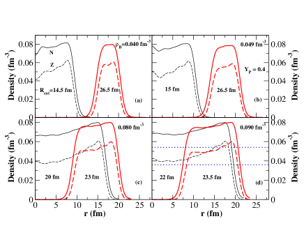
Figure 2: (Color online) The neutron (solid line) and proton (dash line) density distributions for the Wigner-Seitz cells with baryon densities of $\rho_{B}$ = 0.040 (a), 0.049 (b), 0.080 (c), and 0.090 fm^-3 (d). The proton fraction is $Y_{p}=0.4$ and $T$ = 1 MeV. The red curves give density distributions for shell states. The black curves give density distributions for nucleus states. The corresponding cell radii are shown in each panel. The dotted lines in the lower right panel are neutron (upper) and proton (lower) densities for uniform matter.

There is an intuitive interpretation of shell states by considering the competition between the surface and Coulomb energies. When the Coulomb energy is more than half of the surface energy, the nucleus can decrease its Coulomb energy, via increasing its average radius and surface area, so that it minimizes the total energy. One possibility is to push the nucleons out spherically and form a shell shape. Note, this change is possible even if one assumes spherical symmetry. The nucleus could also deform its shape to a non-spherical configuration to minimize the total energy. It may be that, for very neutron rich matter in certain regions of density, the most stable configuration is non-spherical Gogelein . Therefore shell states may be related to the appearance of complex pasta phases pasta ; crust1 ; Gogelein . Perhaps one can think of shell states as “spherical pasta”.

To get a more quantitative idea for the appearance of shell states, we consider a simple model. Suppose there is a spherical WS cell with average baryon density $\rho_{B}$ = 0.071 fm^-3 and $Y_{p}$ = 0.5. Assume the nucleons have a uniform density equal to the saturation nuclear density. There can be either a uniform density nucleus or a uniform density shell state with a hole in the center. The schematic model is shown in the upper panel of Fig. 3. The relevant contributions to the energy are the surface and Coulomb energies. For each fixed WS cell radius, the radius of the outside, and perhaps inside surface of the nucleus can be adjusted to minimize the total energy. By this procedure of minimization, we can get the Coulomb energy, surface energy, and total energy of the cell for a range of cell radii as shown in the lower panel of Fig. 3. When the cell radius is small, the configuration minimizing the total energy is that of a normal nucleus. When the cell radius increases, so that the Coulomb energy is larger than half of the surface energy, the nucleons will be pushed out from the center by Coulomb repulsion and form a shell. This transition decreases the Coulomb energy while the surface energy is increased. For large WS radii, the change in Coulomb energy dominates over the change in surface energy and the total energy of the cell will decrease. Therefore the appearance of a shell state reduces the Coulomb energy and minimizes the total energy at the expense of a larger surface energy. Now there are two minima in the total energy as a function of WS cell radius. The nucleus state has a radius of 12.52 fm and has ${}^{A}Z$ =${}^{584}292$. The shell state has a radius of 20.08 fm and ${}^{A}Z$= ${}^{2408}1204$. Here the shell state is more stable since it has a lower energy.

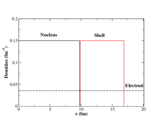
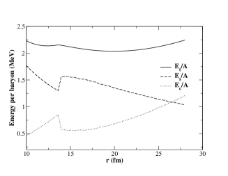
Figure 3: (Color online) Upper panel: nucleon density distributions for nucleus (solid black curve) and shell state (solid red curve) in a schematic model for WS cell with $\rho_{B}$ = 0.071 fm^-3 and $Y_{p}$ = 0.5; dotted line is electron density. Lower panel: the total energy per baryon $E_{t}/A$, surface energy per baryon $E_{s}/A$ and Coulomb energy per baryon $E_{c}/A$ versus WS cell radius, with the same conditions as above.

There may be a similar situation for super heavy nuclei. For the predicted doubly magic nucleus ${}^{292}120$, different mean field model calculations show central depressions in the nuclear density heavy . The shell state we find can be considered as an even larger super heavy nucleus with a central depression: the Coulomb repulsion is so large that the protons are pushed out from the center completely and locate in the outer region of the cell. Note that the neutrons then follow the protons in order to reduce the symmetry energy.

In Fig. 4, the atomic $A$ and proton $Z$ numbers for nucleus and shell states (upper panel), and the corresponding WS cell radii (lower panel) are shown as functions of the baryon density. The proton fraction is $Y_{p}$ = 0.4. At low baryon densities, the WS cell radius of the shell state is about twice that of the nucleus state, e.g., 26 fm vs. 14 fm at $\rho_{B}$ = 0.040 fm^-3. The cell radii of shell states decrease with increasing density, while those of nucleus state increase with density. They approach one another at high baryon densities: 24 fm vs. 22 fm at 0.090 fm^-3. For both nucleus and shell states, $A$ and $Z$ increase with increasing baryon density.

In the upper panel of Fig. 5, the free energy per baryon for non-uniform matter (both nucleus state and shell state) and uniform matter are shown as function of densities with $Y_{p}$ = 0.4. In the lower panel, the free energy difference between the nucleus and shell states is shown for various baryon densities. This difference is of order tens of KeV and is maximum around 0.070 fm^-3. When the baryon density $\rho_{B}<$ 0.049 fm^-3, the nucleus state is the most stable. Between densities of 0.049 to 0.090 fm^-3, the shell state becomes slightly more stable than the nucleus state. When $\rho_{B}>$ 0.090 fm^-3, the matter becomes uniform.

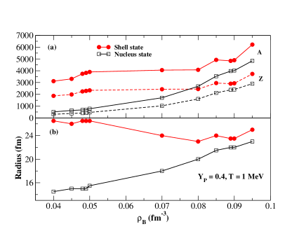
Figure 4: (Color online) The atomic and proton numbers (panel a), and the WS cell radii for nucleus (squares) and shell states (filled circles) (panel b) shown as functions of the baryon density for $Y_{p}$ = 0.4.

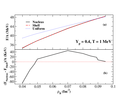
Figure 5: (Color online) Upper panel (a): the free energy per baryon for non-uniform matter, nucleus (solid line) and shell states (dot-dash line), and uniform matter (dashed line) are shown as function of the baryon density for $Y_{p}$ = 0.4 and $T$ = 1 MeV. Lower panel (b): free energy difference per baryon between nucleus and shell states versus baryon density.

The above analysis for $Y_{p}$ = 0.4 can be generalized for different proton fractions $Y_{p}$. For $Y_{p}$ = 0.5, the minimization of free energy per baryon over the WS cell radii with baryon density of 0.045, 0.053, 0.073, and 0.090 fm^-3 are shown in Fig. 6. Again there are two minima corresponding to nucleus state and shell state respectively. The neutron and proton density distributions associated with the two states are shown in Fig. 7. The transition density from nucleus state to shell state is 0.053 fm^-3. In Fig. 8, the atomic and proton numbers (upper panel), and the WS cell radii (lower panel) for nucleus state and shell state are shown for various baryon densities. In Fig. 9, the free energy per baryon for non-uniform matter (both nucleus state and shell state) and uniform matter are shown as function of densities. When the baryon density is smaller than 0.053 fm^-3, the nucleus state is the most favorable state. Between 0.053 to 0.090 fm^-3, the shell state become slightly more stable than the nucleus state. When the density is above 0.090 fm^-3 (same as that when $Y_{p}$ = 0.4), the uniform matter is the stable state.

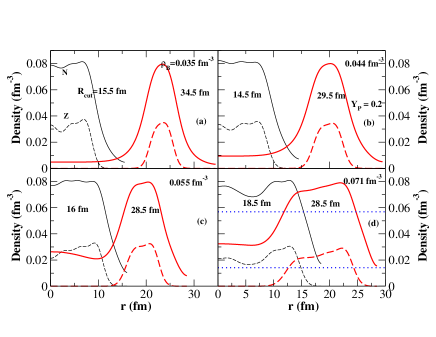
Figure 15: (Color online) The neutron (solid line) and proton (dashed line) density distributions for the Wigner-Seitz cells at baryon densities of $\rho_{B}$ = 0.035, 0.044, 0.055 and 0.071 fm^-3, with proton fraction $Y_{p}=0.2$ and $T$ = 1 MeV. The red curves give density distributions of shell states. The black curves give density distributions of nuclear states. The corresponding cell radii are shown in each panel. The dotted lines in the lower right panel are the neutron (upper) and proton (lower) densities of uniform matter.

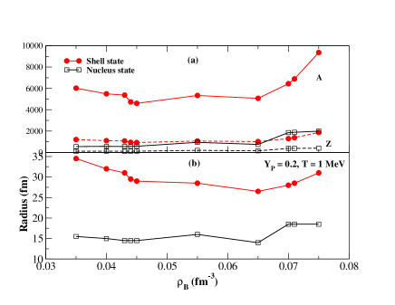
Figure 16: (Color online) The upper panel (a) shows atomic (solid line) and proton (dashed line) numbers, while the lower panel (b) shows WS cell radii, for nucleus (squares) and shell states (filled circles) as functions of the baryon density for $Y_{p}$ = 0.2.

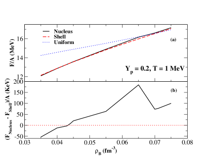
Figure 17: (Color online) Upper panel (a): the free energy per baryon for non-uniform matter, nucleus (solid line) and shell state (dot-dashed line), and uniform matter (dashed line) are shown as function of density with $Y_{p}$ = 0.2 and $T$ = 1 MeV. Lower panel (b): free energy difference per baryon between the nucleus and shell states versus baryon density.

Similar calculations were carried out for $Y_{p}$ = 0.3 and the results are presented in Figs. 10, 11, 12 and 13. We note that the transition density to the shell state is 0.043 fm^-3 and the transition density to uniform matter is 0.084 fm^-3. For $Y_{p}$ = 0.2, the results are presented in Figs. 14, 15, 16 and 17. The transition density to shell state is 0.044 fm^-3 and to uniform matter is 0.071 fm^-3. The matter is very neutron rich at $Y_{p}$ = 0.2 and the nucleon density distributions of shell states have a distinct feature, compared to results for $Y_{p}$ = 0.3, 0.4, and 0.5. The neutron densities are not vanishing in the center and on the edge of the shell nuclei, as shown in Fig. 15. The neutron chemical potential is greater than zero. Therefore there are appreciable numbers of free neutrons inside the cell.

Comparison between Fig. 9 and Fig. 17 indicates that shell states will start to appear at smaller density for smaller $Y_{p}$. Shell states involve a competition between surface and Coulomb energies. Neutron rich matter, with only a few protons, has a small binding energy and therefore a small surface energy. This small surface energy makes it easier to form shell states. Furthermore, we notice that at smaller $Y_{p}$ the transition to uniform matter appears at smaller density. So in fact the density range for the shell state has decreased for smaller $Y_{p}$.

Up to now, we have examined the EOS in the WS approximation for nonuniform and uniform nuclear matter with $Y_{p}$ = 0.2, 0.3, 0.4, and 0.5. A universal picture of phase transitions from normal nuclei to shell nuclei, then to uniform matter with increasing baryon densities emerges. It is beneficial to quantitatively compare the results to other analytical methods. As presented in Section. II.2, using the eigencondition $D(\Omega=0)=0$ from the semiclassical collective mode analysis and Eq. (44) from the finite temperature RPA analysis respectively, one can obtain the phase transition density to uniform matter. In Fig. 18, the phase transition densities to uniform matter at $T$ = 1 MeV are shown for different proton fractions. The transition densities obtained from the above two analyses are plotted in comparison with the Hartree WS calculations. At $Y_{P}$ = 0.3, these two analyses give the transition density close to the WS approximation. When $Y_{P}>$ 0.3, the two analyses give slightly smaller transition densities. When $Y_{P}<$ 0.3, the two analyses give bigger transition densities. The latter difference may suggest existence of non-spherical configurations in the region between the spherical WS transition density and the collective modes/RPA transition density for non-uniform neutron rich matter.

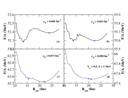
Figure 6: (Color online) Free energy per baryon versus Wigner-Seitz cell radius for baryon densities of $\rho_{B}$ = 0.045, 0.053, 0.073, and 0.090 fm^-3, proton fraction $Y_{p}=0.5$ and $T$ = 1 MeV. The two open circles denote minima corresponding to the nucleus (left) and shell (right) states.

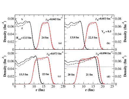
Figure 7: (Color online) The neutron (solid line) and proton (dash line) density distributions for the Wigner-Seitz cells with baryon density $\rho_{B}$ = 0.045, 0.053, 0.073, and 0.090 fm^-3, with proton fraction $Y_{p}=0.5$ and $T$ = 1 MeV. The red curves give density dist. of shell state. The black curves give density dist. of nucleus state. The corresponding cell radii are shown in each panel. The dotted line in the lower right panel is the neutron or proton density of uniform matter.

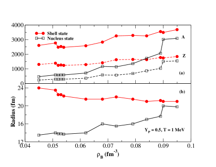
Figure 8: (Color online) The upper panel (a) shows atomic (solid line) and proton (dashed line) numbers, while the lower panel (b) shows WS cell radii, for nucleus (squares) and shell states (filled circles) as functions of the baryon density for $Y_{p}$ = 0.5.

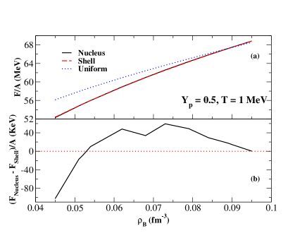
Figure 9: (Color online) Upper panel (a): the free energy per baryon for non-uniform matter, nucleus (solid line) and shell state (dot-dashed line), and uniform matter (dashed line) are shown as functions of density for $Y_{p}$ = 0.5 and $T$ = 1 MeV. Lower panel (b): free energy difference per baryon between nucleus and shell states versus baryon density.

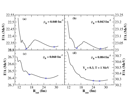
Figure 10: (Color online) Free energy per baryon versus Wigner-Seitz cell radii for baryon densities of $\rho_{B}$ = 0.040, 0.043, 0.060, and 0.084 fm^-3, proton fraction $Y_{p}=0.3$ and $T$ = 1 MeV. The two open circles denote minima corresponding to nucleus (left) and shell (right) states.

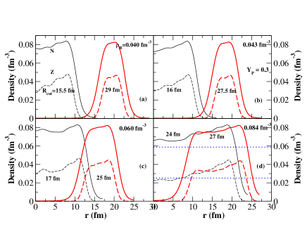
Figure 11: (Color online) The neutron (solid line) and proton (dash line) density distributions for the Wigner-Seitz cells at baryon densities of $\rho_{B}$ = 0.040, 0.043, 0.060, and 0.084 fm^-3, for proton fraction $Y_{p}=0.3$ and $T$ = 1 MeV. The red curves give density distributions for shell states. The black curves give density distributions of nucleus states. The corresponding cell radii are shown in each panel. The dotted lines in the lower right panel are the neutron (upper) and proton (lower) density of uniform matter.

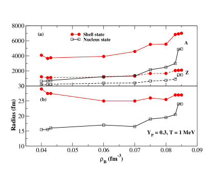
Figure 12: (Color online) The upper panel (a) shows atomic (solid line) and proton (dashed line) numbers, while the lower panel (b) shows WS cell radii, for nucleus (squares) and shell states (filled circles) as functions of the baryon density for $Y_{p}$ = 0.3.

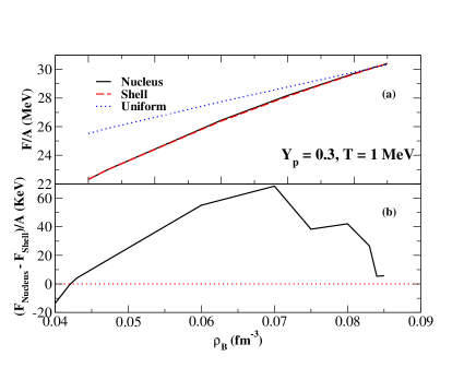
Figure 13: (Color online) Upper panel (a): the free energy per baryon for non-uniform matter, nucleus (solid line) and shell state (dot-dashed line), and uniform matter (dashed line) are shown as functions of density for $Y_{p}$ = 0.3 and $T$ = 1 MeV. Lower panel (b): free energy difference per baryon between nucleus and shell states versus baryon density.

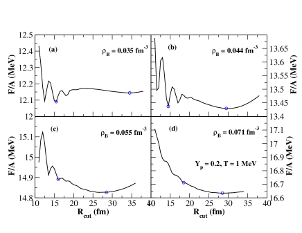
Figure 14: (Color online) Free energy per baryon versus Wigner-Seitz cell radius for baryon densities of $\rho_{B}$ = 0.035, 0.044, 0.055, and 0.071 fm^-3, proton fraction $Y_{p}=0.2$ and $T$ = 1 MeV. The two open circles denote minima of nucleus (left) and shell (right) states.

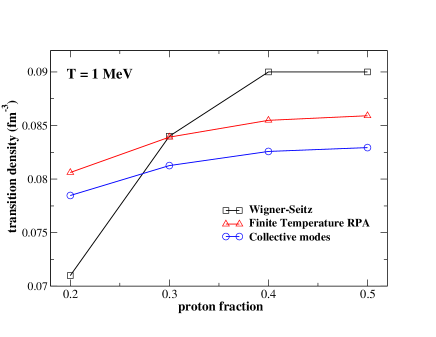
Figure 18: (Color online) The phase diagram for nuclear matter at $T$ = 1 MeV and different proton fractions, combining results from Wigner-Seitz cell calculation, collective modes analysis and RPA at finite temperature.

IV Summary

In this paper we applied a Relativistic Mean Field model to study the equation of state for non-uniform and uniform nuclear matter over a large range of baryon densities and with proton fractions, $Y_{p}$ = 0.2, 0.3, 0.4 and 0.5. Within the spherical Wigner-Seitz approximation for non-uniform nuclear matter, we studied the system at a low temperature, $T$ = 1 MeV. We find new shell states which minimize the free energy over a significant range of baryon densities. These shell states minimize the Coulomb energy of configurations with many protons at the expense of a larger surface energy. These states are related to a possible central depression in the density distribution of super heavy nuclei. As the density increases, the system undergoes phase transitions from normal nuclei to shell states, and then to uniform matter.

We compared our Wigner-Seitz results to two stability analyses of uniform nuclear matter. Here we looked at collective modes in the RMF plus Vlasov formalism and in the finite temperature RPA. The two analyses agree well with each other and give a slightly lower transition density to uniform matter at large proton fractions ($Y_{p}=0.5$, 0.4), and a higher transition density at small proton fractions (below 0.3) compared to the WS results. This latter difference may suggest the existence of non-spherical configurations in the density region between the spherical WS transition density and the collective modes/RPA transition density for non-uniform neutron rich matter.

We conclude that even in a spherical approximation, there are more possible configurations than have been previously considered. These new shell states may play a role in the thermal and quantum fluctuations of the system and in its response to a variety of probes. Furthermore these shell states may allow one to include, in a simple way, much of the physics of, potentially complicated, non-spherical pasta configurations.

In this investigation pairing between nucleons is not included, since it is expected to have only a small effect on bulk properties such as the pressure or free energy. However the effects of pairing on transport properties remains to be investigated. In the future, we will study the equation of state at higher temperatures and investigate the response of shell states to supernova neutrinos. We will also study the system at smaller proton fractions appropriate for neutron star matter in beta equilibrium. Our ultimate goal is to produce an equation of state spanning a more complete range of baryon densities, temperatures, and proton fractions, that will be suitable for astrophysical applications to neutron stars and supernovae.

V acknowledgement

We thank Brian Serot for helpful discussions and Don Berry for help with a computer cluster at Indiana University. This work was supported in part by DOE grant DE-FG02-87ER40365.

References

- (1) See for example C. Hartnack et al., Phys. Rev. Lett. 96, 012302 (2006). P. Danielewicz, R. Lacey, and W. G. Lynch, Science 22, 1592 (2002).
- (2) See for example S. Bogdanov et al., arXiv:0801.4030. N. A. Webb and D. Barret, arXiv:0708.3816.
- (3) J. W. Negele and D. Vautherin, Nucl. Phys. A 207, 298 (1973).
- (4) See for example T. Maruyama et al., Phys. Rev. C72, 015802 (2005).
- (5) D. G. Ravenhall, C. J. Pethick, and J. R. Wilson, Phys. Rev. Lett. 50, 2066 (1983).
- (6) C. P. Lorenz, D. G. Ravenhall, and C. J. Pethick, Phys. Rev. Lett. 70, 379 (1993).
- (7) C. J. Horowitz, M. A. Pérez-García, and J. Piekarewicz, Phys. Rev. C 69, 045804 (2204).
- (8) J. M. Lattimer and F. D. Swesty, Nucl. Phys. A 535, 331 (1991).
- (9) H. Shen, H. Toki, K. Oyamatsu, and K. Sumiyoshi, Nucl. Phys. A 637, 435 (1998).
- (10) C. J. Horowitz and B. D. Serot, Nucl. Phys. A 368, 503 (1981).
- (11) C. J. Horowitz and B. D. Serot, Phys. Lett. B 86, 146 (1979).
- (12) B. D. Serot and J. D. Walecka, Adv. Nucl. Phys. 16, 1 (1986).
- (13) P.-G. Reinhard, Rep. Prog. Phys. 52, 439 (1989).
- (14) P. Ring, Prog. Part. Nucl. Phys. 37, 193 (1996).
- (15) C. Kittel, Introduction to Solid State Physics, P. 571, John Wiley & Sons Inc, 2nd Edition (1956).
- (16) K. Oyamatsu, M. Hashimoto and M. Yamada, Prog. Theor. Phys. 72, 373 (1984).
- (17) L. Brito, C. Providencia, A. M. Santos, S. S. Avancini, D. P. Menezes, and Ph. Chomaz, Phys. Rev. C 74, 045801 (2006).
- (18) C. J. Horowitz and K. Wehrberger, Phys. Lett. B 266, 236 (1991).
- (19) A. V. Afanasjev, S. Frauendorf, Phys. Rev. C 71, 024308 (2005) .
- (20) G. A. Lalazissis, J. König, and P. Ring, Phys. Rev. C55, 540 (1997).
- (21) See for example P. Gögelein, E. N. E. van Dalen, C. Fuchs, and H. Müther, Phys. Rev. C 77, 025802 (2008).
- (22) H. Sonoda et al., Phys. Rev. C77, 035806 (2008). C. J. Horowitz et al., Phys. Rev. C70, 065806 (2004).