The Remarkable Simplicity of Very High Dimensional Data: Application of Model-Based Clustering

Fionn Murtagh Department of Computer Science, Royal Holloway, University of London, Egham TW20 0EX, England. fmurtagh@acm.org

Abstract

An ultrametric topology formalizes the notion of hierarchical structure. An ultrametric embedding, referred to here as ultrametricity, is implied by a hierarchical embedding. Such hierarchical structure can be global in the data set, or local. By quantifying extent or degree of ultrametricity in a data set, we show that ultrametricity becomes pervasive as dimensionality and/or spatial sparsity increases. This leads us to assert that very high dimensional data are of simple structure. We exemplify this finding through a range of simulated data cases. We discuss also application to very high frequency time series segmentation and modeling.

Keywords: multivariate data analysis, cluster analysis, hierarchy, ultrametric, p-adic, dimensionality

1 Introduction

The lessons we will draw from this work are as follows.

•

Very high dimensional spaces are of very simple structure.
•

It becomes easier to find clusters in high dimensions.
•

The simple high dimensional structure is hierarchical.
•

Ease of handling high dimensional data, e.g. reading off clusters, emulates the human perception system which similarly processes data with no evident latency.

There is a burgeoning crisis in high dimensional data analysis, and many current approaches lack convincing performance guarantees. In Hinneburg, Aggarwal and Keim (2000), attention is focused on “relevant” dimensions only, while Aggarwal, Hinneburg and Keim (2001) (cf. the revealing titles in the case of both of these citations) state: “Recent research results show that in high dimensional space, the concept of proximity, distance or nearest neighbor may not even be qualitatively meaningful.” The last-mentioned work investigates $L_{p}$ norms including for fractional values of $p$ .

In Breuel (2007), the focus is the $\epsilon$ -approximate nearest neighbor defined as follows: if the nearest neighbor point $y$ to some query point, $x$ , has distance $d(x,y)$ , then any vector $y^{\prime}$ such that $d(y^{\prime},x)\leq(1+\epsilon)d(x,y)$ is an $\epsilon$ -approximate nearest neighbor of $x$ . Then Breuel (2007) points out: “… the relationship between approximation and ’cost’ of a solution need not be linear. For example, the cost of picking an $\epsilon$ -approximate nearest neighbor could be proportional not to the difference of distances between the optimal answer and the approximation, but to the volume of the shell between the two, that is, as $(1+\epsilon)^{m-1}$ , where $m$ is the dimension of the space.” Various issues immediately ensue: (i) “for large dimensions, even small values of $\epsilon$ include the entire database as $\epsilon$ -approximate neighbors”; (ii) “analyzing the worst-case asymptotic complexity of $\epsilon$ -approximate algorithms is meaningless”; (iii) for “large enough dimensions, a randomly chosen point becomes an $\epsilon$ -approximate nearest neighbor with high probability”; (iv) “the implicit assumption that a close approximation leads to only a small increase in the cost of a solution is not justifiable in the context of nearest neighbors”; and (v) an $\epsilon$ -approximate nearest neighbor algorithm is not necessarily useless in practice but such an algorithm has “neither useful meaning asymptotically (as the dimension grows), nor does it make useful predictions about its behavior on practical problems”.

In this article, we propose an approach which we consider appropriate for high dimensional data analysis, based on clustering and proximity searching.

1.1 The Ultrametricity Perspective and Overview of this Work

The morphology or inherent shape and form of an object is important. In data analysis, the inherent form and structure of data clouds are important. So the embedding topology, with which the data clouds are studied, can be crucial. Quite a few models of data form and structure are used in data analysis. One of them is a hierarchically embedded set of clusters, – a hierarchy. It is traditional (since at least the 1960s) to impose such a form on data, and if useful to assess the goodness of fit. Rather than fitting a hierarchical structure to data (e.g., Rohlf and Fisher, 1968), our recent work has taken a different orientation: we seek to find (partial or global) inherent hierarchical structure in data. As we will describe in this article, there are interesting findings that result from this, and some very interesting perspectives are opened up for data analysis and, potentially, perspectives also on the physics (or causal or generative mechanisms) underlying the data.

A formal definition of hierarchical structure is provided by ultrametric topology (in turn, related closely to p-adic number theory). We will return to this in section 2 below. First, though, we will summarize some of our findings.

Ultrametricity is a pervasive property of observational data. It arises as a limit case when data dimensionality or sparsity grows. More strictly such a limit case is a regular lattice structure and ultrametricity is one possible representation for it. Notwithstanding alternative representations, ultrametricity offers computational efficiency (related to tree depth/height being logarithmic in number of terminal nodes), linkage with dynamical or related functional properties (phylogenetic interpretation), and processing tools based on well known p-adic or ultrametric theory (examples: deriving a partition, or applying an ultrametric wavelet transform). In Khrennikov (1997) and other works, Khrennikov has pointed to the importance of ultrametric topological analysis.

Local ultrametricity is also of importance. This can be used for forensic data exploration (fingerprinting data sets): see Murtagh (2005, 2007); and to expedite search and discovery in information spaces: see Chávez, Navarro, Baeza-Yates and Marroquín (2001) as discussed by us in Murtagh (2004, 2006) and Murtagh, Downs and Contreras (2007).

In section 2 we show how extent of ultrametricity is measured. Section 3 presents our main results on the remarkable properties of very high dimensional, or very sparse, spaces. As dimensionality or sparsity grow, so does the inherent hierarchical nature of the data in the space. In section 4 we then discuss application to very high frequency time series modeling.

1.2 Review of Recent Asymptotic Statistical Findings

We can characterize clustering algorithms in terms of number of observables, $n$ , and number of attributes, $m$ , where by “large” is meant thousands upwards: (i) large $n$ , small $m$ ; as is fairly standard in astronomy; (ii) large $n$ , large $m$ ; as is fairly typically the case in information retrieval; and (iii) small $n$ , large $m$ ; as is often the case in bioinformatics, and textual forensics. It is case (iii) which is of most interest to us here. However our results also accommodate case (ii).

In Hall, Marron and Neeman (2005), it was shown that “under some conditions on underlying distributions, as the dimension tends to infinity with a fixed sample size, the $n$ data vectors form a regular $n$ -simplex in $\mathbb{R}^{m}$ ” (Ahn, Marron, Muller and Chi, 2007). These authors term the small $n$ , large $m$ case “HDLSS, high dimension, low sample size”. In Ahn and Marron (2005), some other unrelated work is cited, where the ratio of $m/n$ tends to a constant. As with these authors, our goal is to study the case of letting “ $m$ tend to infinity, fixing $n$ ” (Ahn and Marron, 2005). Hall et al. (2005) discuss previous asymptotics work in the statistical literature. Our focus is not on a simplex but rather on a hierarchy (even if trivial) in order to study implications for data analysis.

For “the asymptotic geometric representation of HDLSS data”, it is shown in the work of Ahn and collaborators that “when $m>>n$ , under a mild assumption, the pairwise distances between each pair of data points are approximately identical so that the data points form a regular $n$ -simplex. In a binary classification setting, the training data from each class becomes two simplices … any reasonable classification method will find the same [discriminant result] when $m$ becomes very large.” (Ahn et al., 2007). This is a very exciting for the discriminant analysis case pursued by Ahn et al., 2007; Ahn and Marron, 2005; Hall et al., 2005) (naive Bayes, SVM or support vector machine, Fisher’s linear discriminant, and the simplex structure in very high dimensions leading to the “direction of maximal data piling”). In this paper, our interest is in clustering, or unsupervised classification.

The mild condition for simplex structure formation, as $m\longrightarrow\infty$ is that directionality of the Gaussian cloud is “diffuse”, defined in terms of eigenvalues:

\sum^{m}_{j}\lambda_{j}^{2}/\left(\sum^{m}_{j}\lambda_{j}\right)^{2}\longrightarrow 0\mbox{ as }m\longrightarrow\infty

Then it is shown that the covariance matrix approaches a constant times the identity matrix.

In Donoho and Tanner (2005), the Gaussian case is also focused on. For a Gaussian cloud, “not only are the points on the convex hull, but all reasonable-sized subsets span faces of the convex hull”. Intuitively, if all points fly apart from one another as dimensionality grows, then (i) each point is a vertex of the convex hull of the cloud of points; (ii) each pair of points generates an edge of the convex hull; and (iii) sets of points form a regional face of the convex hull. These properties are proven by Donoho and Tanner (2005) who conclude: “This is wildly different than the behavior that would be expected by traditional low-dimensional thinking.”

We may ask why we (in this work) lay importance on the fact that the high dimensional simplex additionally defines an ultrametric topological embedding. An ultrametric topology requires (as will be described in sections to follow) any triangle to be either (i) equilateral, or (ii) isosceles with small base. The equilateral case corresponds fine with the simplex structure. But it is useful to us to hang on to the isosceles with small base case, too, for inter-cluster relationships. We will look later at examples to support this viewpoint.

2 Quantifying Degree of Ultrametricity

Summarizing a full description in Murtagh (2004) we explored two measures quantifying how ultrametric a data set is, – Lerman’s and a new approach based on triangle invariance (respectively, the second and third approaches described in this section).

The triangular inequality holds for a metric space: $d(x,z)\leq d(x,y)+d(y,z)$ for any triplet of points $x,y,z$ . In addition the properties of symmetry and positive definiteness are respected. The “strong triangular inequality” or ultrametric inequality is: $d(x,z)\leq\mbox{ max }\{d(x,y),d(y,z)\}$ for any triplet $x,y,z$ . An ultrametric space implies respect for a range of stringent properties. For example, the triangle formed by any triplet is necessarily isosceles, with the two large sides equal; or is equilateral.

•

Firstly, Rammal, Toulouse and Virasoro (1986) used discrepancy between each pairwise distance and the corresponding subdominant ultrametric. Now, the subdominant ultrametric is also known as the ultrametric distance resulting from the single linkage agglomerative hierarchical clustering method. Closely related graph structures include the minimal spanning tree, and graph (connected) components. While the subdominant provides a good fit to the given distance (or indeed dissimilarity), it suffers from the “friends of friends” or chaining effect.
•

Secondly, Lerman (1981) developed a measure of ultrametricity, termed H-classifiability, using ranks of all pairwise given distances (or dissimilarities). The isosceles (with small base) or equilateral requirements of the ultrametric inequality impose constraints on the ranks. The interval between median and maximum rank of every set of triplets must be empty for ultrametricity. We have used extensively Lerman’s measure of degree of ultrametricity in a data set. Taking ranks provides scale invariance. But the limitation of Lerman’s approach, we find, is that it is not reasonable to study ranks of real-valued (values in non-negative reals) distances defined on a large set of points.
•

Thirdly, our own measure of extent of ultrametricity (Murtagh, 2004) can be described algorithmically. We examine triplets of points (exhaustively if possible, or otherwise through sampling), and determine the three angles formed by the associated triangle. We select the smallest angle formed by the triplet points. Then we check if the other two remaining angles are approximately equal. If they are equal then our triangle is isosceles with small base, or equilateral (when all triangles are equal). The approximation to equality is given by 2 degrees (0.0349 radians). Our motivation for the approximate (“fuzzy”) equality is that it makes our approach robust and independent of measurement precision.

A supposition for use of our measure of ultrametricity is that we can define angles (and hence triangle properties). This in turn presupposes a scalar product. Thus we presuppose a complete normed vector space with a scalar product – as one example, the real part of a Hilbert space – to provide our needed environment.

Quite a general way to embed data, to be analyzed, in a Euclidean space, is to use correspondence analysis (Murtagh, 2005). This explains our interest in using correspondence analysis: it provides a convenient and versatile way to take input data in many varied formats (e.g., ranks or scores, presence/absence, frequency of occurrence, and many other forms of data) and map them into a Euclidean, factor space.

3 Ultrametricity and Dimensionality

3.1 Distance Properties in Very Sparse Spaces

Murtagh (2004), and earlier work by Rammal, Angles d’Auriac and Doucot (1985) and Rammal et al. (1986), has demonstrated the pervasiveness of ultrametricity, by focusing on the fact that sparse high-dimensional data tend to be ultrametric. In such work it is shown how numbers of points in our clouds of data points are irrelevant; but what counts is the ambient spatial dimensionality. Among cases looked at are statistically uniformly (hence “unclustered”, or without structure in a certain sense) distributed points, and statistically uniformly distributed hypercube vertices (so the latter are random 0/1 valued vectors). Using our ultrametricity measure, there is a clear tendency to ultrametricity as the spatial dimensionality (hence spatial sparseness) increases.

As Hall et al. (2005) also show, Gaussian data behave in the same way and a demonstration of this is seen in Table 1. To provide an idea of consensus of these results, the 200,000-dimensional Gaussian was repeated and yielded on successive runs values of the ultrametricity measure of: 0.96, 0.98, 0.96.

No. points	Dimen.	Isosc.	Equil.	UM
Uniform
100	20	0.10	0.03	0.13
100	200	0.16	0.20	0.36
100	2000	0.01	0.83	0.84
100	20000	0	0.94	0.94
Hypercube
100	20	0.14	0.02	0.16
100	200	0.16	0.21	0.36
100	2000	0.01	0.86	0.87
100	20000	0	0.96	0.96
Gaussian
100	20	0.12	0.01	0.13
100	200	0.23	0.14	0.36
100	2000	0.04	0.77	0.80
100	20000	0	0.98	0.98

Table 1: Typical results, based on 300 sampled triangles from triplets of points. For uniform, the data are generated on [0, 1]; hypercube vertices are in

\{0,1\}^{m}

, and for Gaussian, the data are of mean 0, and variance 1. Dimen. is the ambient dimensionality. Isosc. is the number of isosceles triangles with small base, as a proportion of all triangles sampled. Equil. is the number of equilateral triangles as a proportion of triangles sampled. UM is the proportion of ultrametricity-respecting triangles (= 1 for all ultrametric).

In the following, we explain why high dimensional and/or sparsely populated spaces are ultrametric. We use the Euclidean distances in the cosine formula to determine angles. Note that there is no averaging of distances involved, nor distances normalized by dimensionality.

As dimensionality grows, so too do distances (or indeed dissimilarities, if they do not satisfy the triangular inequality). The least change possible for dissimilarities to become distances has been formulated in terms of the smallest additive constant needed, to be added to all dissimilarities (Torgerson, 1958; Cailliez and Pagès, 1976; Cailliez, 1983; Neuwirth and Reisinger, 1982; and the comprehensive review of Bénasséni, Bennani Dosse and Joly, 2007). Adding a sufficiently large constant to all dissimilarities transforms them into a set of distances. Through addition of a larger constant, it follows that distances become approximately equal, thus verifying a trivial case of the ultrametric or “strong triangular” inequality. Adding to dissimilarities or distances may be a direct consequence of increased dimensionality.

For a close fit or good approximation, the situation is not as simple for taking dissimilarities, or distances, into ultrametric distances. A best fit solution is given by de Soete (1986) (and software is available in Hornik, 2005). If we want a close fit to the given dissimilarities then a good choice would avail either of the maximal inferior, or subdominant, ultrametric; or the minimal superior ultrametric. Stepwise algorithms for these are commonly known as, respectively, single linkage hierarchical clustering; and complete link hierarchical clustering. (See Benzécri, 1979; Lerman, 1981; Murtagh, 1985; and other texts on hierarchical clustering.)

3.2 No “Curse of Dimensionality” in Very High Dimensions

Bellman’s (1961) “curse of dimensionality” relates to exponential growth of hypervolume as a function of dimensionality. Problems become tougher as dimensionality increases. In particular problems related to proximity search in high-dimensional spaces tend to become intractable.

In a way, a “trivial limit” (Treves, 1997) case is reached as dimensionality increases. This makes high dimensional proximity search very different, and given an appropriate data structure – such as a binary hierarchical clustering tree – we can find nearest neighbors in worst case $O(1)$ or constant computational time (Murtagh, 2004). The proof is simple: the tree data structure affords a constant number of edge traversals.

The fact that limit properties are “trivial” makes them no less interesting to study. Let us refer to such “trivial” properties as (structural or geometrical) regularity properties (e.g. all points lie on a regular lattice).

First of all, the symmetries of regular structures in our data may be of importance. For example, processing of such data can exploit these regularities.

Secondly, “islands” or clusters in our data, where each “island” is of regular structure, may be of interpretational value.

Thirdly, and finally, regularity of particular properties does not imply regularity of all properties. So, for example, we may have only partial existence of pairwise linkages.

Thus we see that in very high dimensions, and/or in very (spatially) sparse data clouds, there is a simplification of structure, which can be used to mitigate any “curse of dimensionality”. Figure 1 shows how the distances within and between clusters become tighter with increase in dimensionality.

Refer to caption — Figure 1: An illustration of how “symmetry” or “structure” can become increasingly pronounced as dimensionality increases. The abscissa shows distance values. Displayed are two simulations, each with 3 sub-populations of Gaussian-distributed data, in, respectively, ambient dimensions of 2000 and 20,000. These simulations correspond to the 3rd last, and 2nd last, rows of Table 1.

3.3 Gaussian Clusters in Very High Dimensions

3.3.1 Introduction

We will distinguish between cluster characteristics as follows:

1.

cluster size: number of points per cluster;
2.

cluster location: here, mean, identical on every dimension;
3.

cluster scale: here, standard deviation, identical on every dimension.

These cluster characteristics are simple ones which serve to exemplify how high dimensional clustering is quite different from analogous problems in low dimensions. In the homogeneous clouds studied in Table 1 it is seen that the isosceles (with small base) case disappeared early on, as dimensionality increased greatly, to the advantage of the equilateral case of ultrametricity. So the points become increasingly equilateral-related as dimensionality grows. This is not the case when the data in clustered, as we will now see.

3.3.2 Clusters with Different Locations, Same Scale

Table 2 is based on two clusters, and shows how isosceles triangles increasingly dominate as dimensionality grows. Figure 2 illustrates low and high dimensionality scenarios relating to Table 2. There is clear confirmation in this table as to how interrelationships in the cluster become more compact and, in a certain sense, more trivial, in high dimensions. This does not obscure the fact that we indeed have hierarchial relationships becoming ever more pronounced as dimensionality, and hence relative sparsity, increase. These observations help us to see quite clearly just how hierachical relationships come about, as ambient dimensionality grows.

No. points	Dimen.	Isosc.	Equil.	UM
200	20	0.08	0	0.08
200	200	0.19	0.04	0.23
200	2000	0.42	0.20	0.62
200	20000	0.74	0.22	0.96
200	20000	0.7	0.28	0.98
200	20000	0.77	0.21	0.98
200	20000	0.76	0.21	0.98
200	20000	0.75	0.24	0.99
200	20000	0.73	0.25	0.98

Table 2: Results based on 300 sampled triangles from triplets of points. Two Gaussian clusters, each of 100 points, were used in each case. One point set was of mean 0, and the other of mean 10, on each dimension. The standard deviations on each dimension were 1 in all cases. Column headings are as in Table 1. Five further results are given for the 20,000-dimension case to show variability.

3.3.3 Clusters with Different Locations, Different Scales

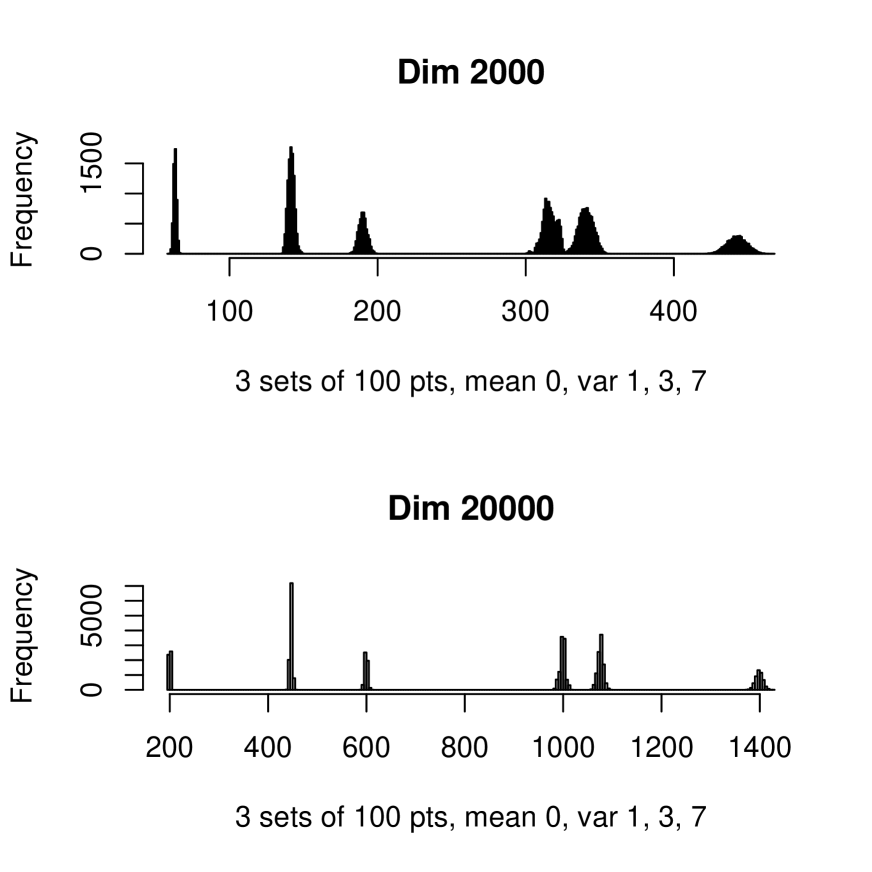
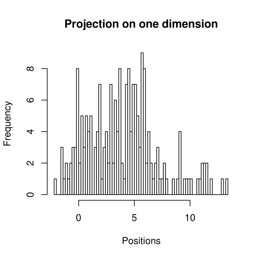
A more demanding case study is now tried. We generate 50 points per cluster with the following characteristics: mean 0, standard deviation 1, on each dimension; mean 3, standard deviation 2, on each dimension; mean 5, standard deviation 1, on each dimension; and mean 8, standard deviation 3, on each dimension. Table 3 shows the results obtained. Here we have not achieved quite the same level of ultrametricty, due to slower growth in ultrametricity which is, in turn, due to the more murky, less dermarcated, but undoubtdely clustered, set of data. Figure 3 illustrates this: this histogram shows one dimension (i.e., one coordinate, chosen arbitrarily), where we note that means of the Gaussians are at 0, 3, 5 and 8.

No. points	Dimen.	Isosc.	Equil.	UM
200	20	0.04	0.01	0.05
200	200	0.11	0.05	0.16
200	2000	0.28	0.06	0.34
200	20000	0.5	0.08	0.58
200	200000	0.55	0.11	0.66

Table 3: Results based on 300 sampled triangles from triplets of points. Four Gaussian clusters, each of 50 points, were used in each case. See text for details of properties of these clusters.

When we look closer at Table 3, as shown in Figure 4, the compaction of distances is again very interesting. We verified the 7 peaks found in the lower histogram in Figure 4, and available but confusedly overlapping and ill-defined in the upper histogram of Figure 4.

What we find for the 7 peaks is as follows. Distances within the clusters correspond to: peaks 1, 2, 3 and (again) 1. That two clusters are associated with one peak is clear from the fact that two of our clusters are of identical scale.

We can examine inter-cluster distances and we found these to be associated with peaks: 2, 3, 4, 5, 6, 7. Given 4 clusters, we could well have up to 6 possible additional peaks.

Were we to be in a far higher dimensional ambient space then we could expect even the inter-cluster distances to become equi-distant.

3.3.4 Identifiability of High Dimensional Gaussian Clouds

From these case studies, it is clear that increased dimensionality sharpens and distinguishes the clusters. If we can embed data – any data – in a far higher ambient dimensionality, without destroying the interpretable relationships in the data, then we can so much more easily read off the clusters.

To read off clusters, including memberships and properties, our findings can be summarized as follows.

For cluster size (i.e., numbers of points per cluster), sampling alone can be used, and we do not pursue this here.

For cluster scale (i.e., standard deviation, assumed the same on each dimension), we associate each cluster, or a pair of clusters, with each peak. The total number of peaks gives an upper bound on the number of clusters. (For $k$ clusters, we have $\leq k+k\cdot(k-1)/2$ peaks.)

Using cluster scale also permits use of the following cluster model: suppose that all clusters are defined to have intra-cluster distance that is less than inter-cluster distance. Then it follows that the peaks of lower distance correspond to the clusters (as opposed to pairs of clusters).

An example of this is as follows. In Figure 4, lower panel, we read from left to right, applying the following algorithm: select the first $k$ peaks as clusters, and ask: are there sufficient peaks to represent all inter-cluster pairs? If we choose $k=3$ , there remain 4 peaks, which is too many to account for the inter-cluster pairs (i.e., $3\cdot(3-1)/2)$ ). So we see that Figure 4 is incompatible with $k=3$ or the presence of just 3 clusters.

Consequently we move to $k=4$ , and see that Figure 4 is consistent with this.

A further identifiability assumption is reasonable albeit not required: that all smallest peaks be associated with intra-cluster distances. This need not be so, since we could well have a dense cluster superimposed on a less dense one. However it is a reasonable parsimony assumption. Supported by this assumption, Figure 4 points to a minimum of 4 clusters in the data, with up to 4 peaks (read off from left to right, i.e., in increasing order of distance) corresponding to these clusters.

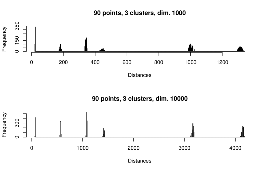
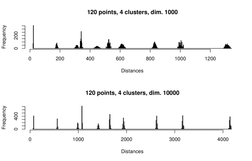
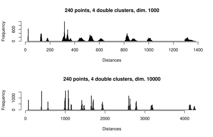
Figure 5 shows peaks, sharpening with rise in ambient dimensionality, for three clusters, distributed as Gaussians with respectively means and standard deviations on all dimensions: (10, 0.5); (0, 4); (40, 10). We see the peaks corresponding to the increasingly similar (and tending towards identical) intra-cluster distances; and then the peaks associated with the 3 inter-cluster distance sets: 6 peaks in total.

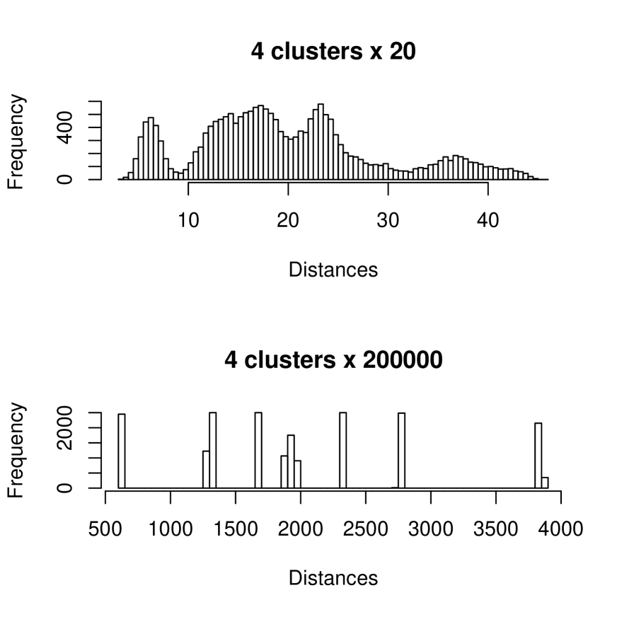
Figure 6 again shows peaks for four clusters, with the same characteristics as for Figure 5, but with an additional cluster of mean and standard deviation on all coordinates: (25, 7). Here we find, as expected, 4 intra-cluster distance peaks, and 6 inter-cluster distance peaks: 10 peaks in total.

The success of cluster identification is clearly dependent on distinguishable intra-cluster properties, which are also distinguishable from the inter-cluster properties.

Figure 7 shows a more tricky case. For the first cluster, the (equally-sized component) distributions had means and standard deviations on all coordinates of: (10, 0.5) and (0, 0.5). For the second cluster, we used: (0, 4) and (10, 4). For the third cluster we used (40, 10) and (0, 10). Finally for the fourth cluster we used the same for all cluster member points: (25, 7). Here, therefore the maximum number of peaks is: for the intra-cluster distances, 2 peaks for the first, second and third clusters, and 1 for the fourth cluster, hence 7. For the inter-cluster distances, assuming the cluster components are close enough, 6, but if they are not, then, we have peaks between essentially 7 clusters, i.e. 21 peaks. Hence in total we could have up to 28 peaks. For the histogram sampling resolution used, we read off, visually, 17 peaks.

Our approach is to have an upper bound on the number of peaks found in the distance histogram. Now we turn to real (or realistic) data and see how this work helps us to address the cluster identifiability problem.

4 Applications

4.1 Application to High Frequency Data Analysis

In this section we establish proof of concept for application of the foregoing work to analysis of very high frequency univariate time series signals.

Consider each of the cases considered in section 3.3, expressed there as $n\times m$ arrays, as instead representing $n$ segments, each of (contiguous) length $m$ , of a time series or one-dimensional signal. Assuming our aim is to cluster these segments on the basis of their properties, then it is reasonable to require that they be non-overlapping. The $n$ segments could come from anywhere, in any order, in the time series. So for the case of an $n\times m$ array considered previously, then implies a time series of length at least $nm$ . The most immediate way to construct the time series is to raster scan the $n\times m$ array, although alternatives come readily to mind.

The methodology discussed in section 3.3 then is seen to be also a time series segmentation approach, facilitating the characterizing of the segments used.

To explore this further we consider a time series consisting of two ARIMA (autoregressive integrated moving average) models, with parameters: order, autoregression coefficients, moving average coefficients, and a “mildly longtailed” set of innovations based on the Student t distribution with 5 degrees of freedom. Figures 8 and 9 show samples of these time series segments. Figures 10 and 11 show histograms of these samples.

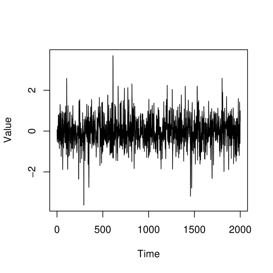
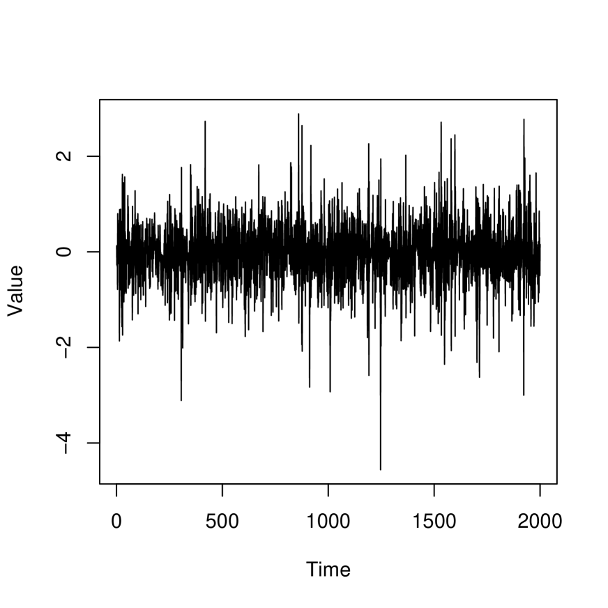
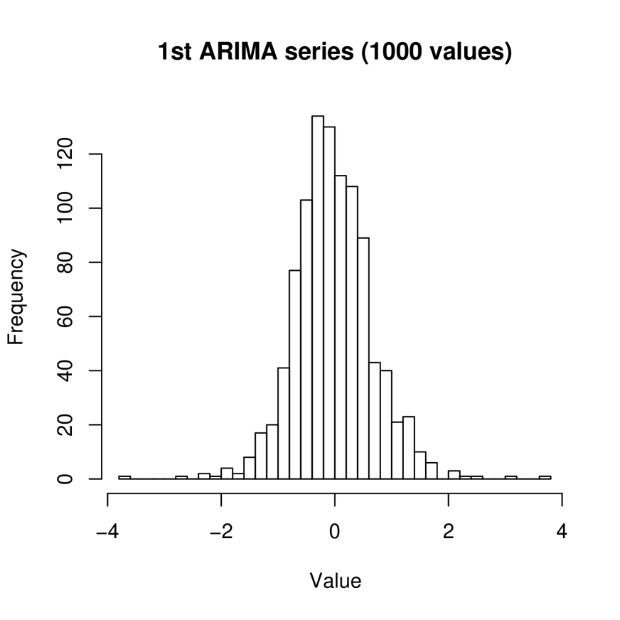
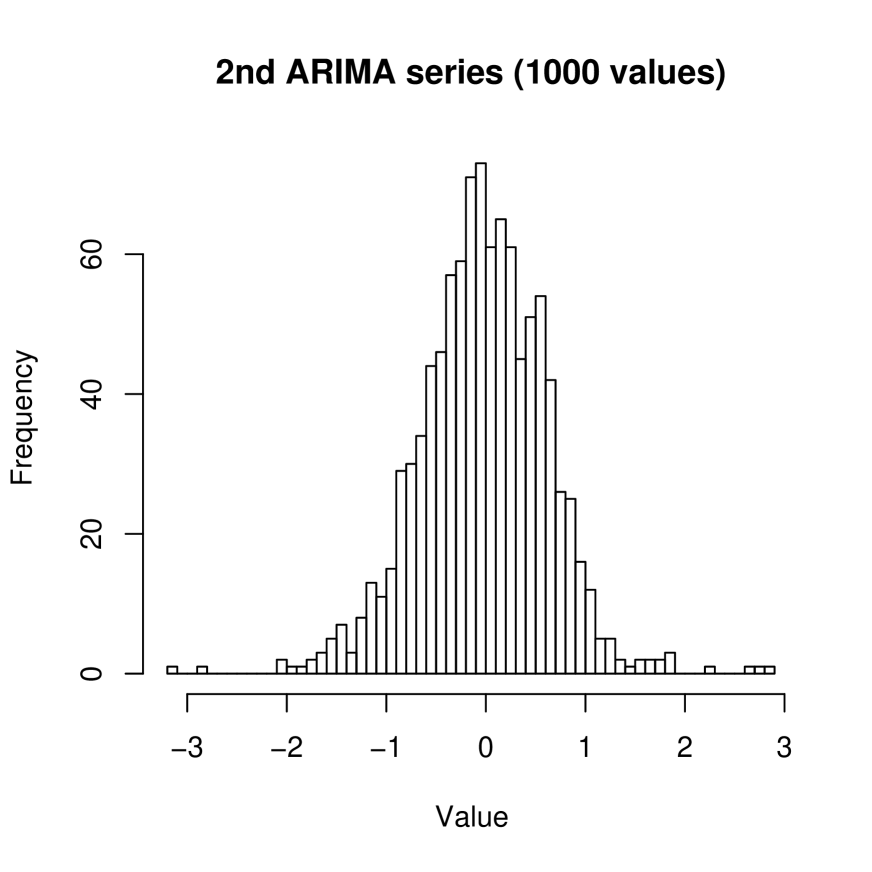
Table 4 shows typical results obtained in regard to ultrametricity. The dimensionality can be considered as the embedding dimension. Here, although ultrametricity increases, and the equilateral configuration seems to be increasing but with decrease of the isosceles with small base configuration, we do not consider it of practical relevance to test with even higher ambient dimensionalities. It is clear from the data, especially Figures 10 and 11, that the two signal models are very close in their properties.

Examining the histograms of all inter-pair time series segments, both intra and inter cluster, we find the clearly distinguished peaks shown in Figure 12. As before, we use Euclidean distance between time series segments or vectors. (We note that normalization or other transformation is not relevant here. In fact we want to distinguish between inter and intra cluster cases. Furthermore the unweighted Euclidean distance is consistent with our use of angles to quantify triangle invariants, and hence respect for ultrametricity properties.)

No. time series	Dimen.	Isosc.	Equil.	UM
100	2000	0.17	0.32	0.49
100	20000	0.15	0.5	0.65
100	200000	0.03	0.57	0.60

Table 4: Results based on 300 sampled triangles from triplets of points. Two sets of the ARIMA models are used, each of 50 realizations.

We find clearly distinguishable peaks in Figure 12. The lower and the higher peaks belong to the two ARIMA components. The central peak belongs to the inter-cluster distances.

We have shown that our methodology can be of use for time series segmentation and for model identifiability. Given the use of a scalar product space as the essential springboard of all aspects of this work, it would appear that generalization of this work to multivariate time series analysis is straightforward. What remains important, however, is the availability of very large embedding dimensionalities, i.e. very high frequency data streams.

4.2 Application in Practice: Segmenting a Financial Signal

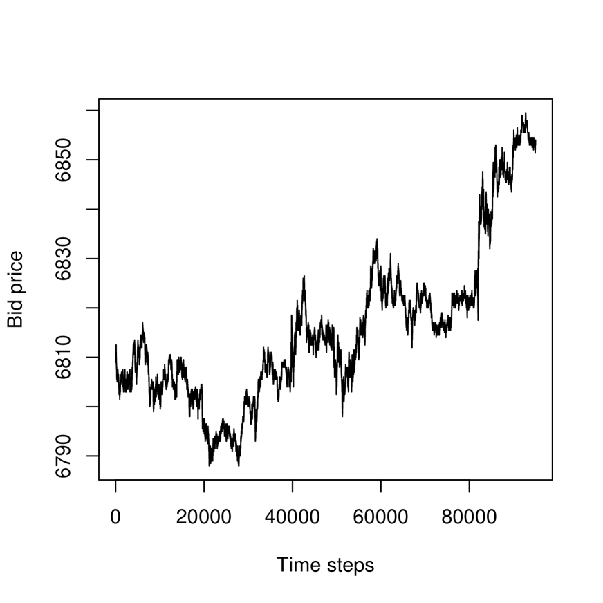
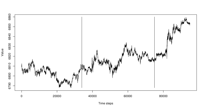
We use financial futures, circa March 2007, denominated in euros from the DAX exchange. Our data stream is at the millisecond rate, and comprises about 382,860 records. Each record includes: 5 bid and 5 asking prices, together with bid and asking sizes in all cases, and action. We extracted one symbol (commodity) with 95,011 single bid values, on which we now report results. See Figure 13.

Embeddings were defined as follows.

•

Windows of 100 successive values, starting at time steps: 1, 1000, 2000, 3000, 4000, $\dots$ , 94000.
•

Windows of 1000 successive values, starting at time steps: 1, 1000, 2000, 3000, 4000, $\dots$ , 94000.
•

Windows of 10000 successive values, starting at time steps: 1, 1000, 2000, 3000, 4000, $\dots$ , 85000.

The histograms of distances between these windows, or embeddings, in respectively spaces of dimension 100, 1000 and 10000, are shown in Figure 14.

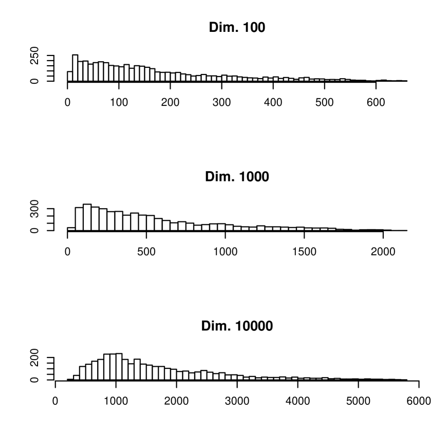
Note how the 10000-length window case results in points that are strongly overlapping. In fact, we can say that 90% of the values in each window are overlapping with the next window. Notwithstanding this major overlapping in regard to clusters involved in the pairwise distances, if we can still find clusters in the data then we have a very versatile way of tackling the clustering objective. Because of the greater cluster concentration that we expect (from discussion in earlier sections of this article) from a greater embedding dimension, we use the 86 points in 10000-dimensional space, notwithstanding the fact that these points are from overlapping clusters.

We make the following supposition based on Figure 13: the clusters will consist of successive values, and hence will be justifiably termed segments.

To validate our approach we will pursue three separate attacks on the same problem of time series segmentation. Firstly, from the distances histogram in Figure 14, bottom, we will carry out Gaussian mixture modeling followed by use of the Bayesian information criterion (BIC, Schwarz, 1978) as an approximate Bayes factor, to determine the best number of clusters (effectively, histogram peaks). Secondly we will use an adjacency-respecting hierarchical clustering algorithm on the full-dimensional (viz., 10000) data. Thirdly, we will use a reduced dimensionality mapping, principal coordinates analysis, using the inter-point distances. Our assumptions in regard to what clusters are present in the data are minimal. Furthermore our validation of segments is based on the three different ways that we have of tackling the one segmentation problem.

We fit a Gaussian mixture model to the data shown in the bottom histogram of Figure 14. To derive the appropriate number of histogram peaks we fit Gaussians and use the Bayesian information criterion (BIC) as an approximate Bayes factor for model selection (Kass and Raftery, 1995; Murtagh and Starck, 2003). Figure 15 shows the succession of outcomes, and indicates as best a 5-Gaussian fit. For this result, we find the means of the Gaussians to be as follows: 517, 885, 1374, 2273 and 3908. The corresponding standard deviations are: 84, 133, 212, 410 and 663. The respective cardinalities of the 5 histogram peaks are: 358, 1010, 1026, 911 and 350. Note that this relates so far only to the histogram of pairwise distances. We now want to determine the corresponding clusters in the input data.

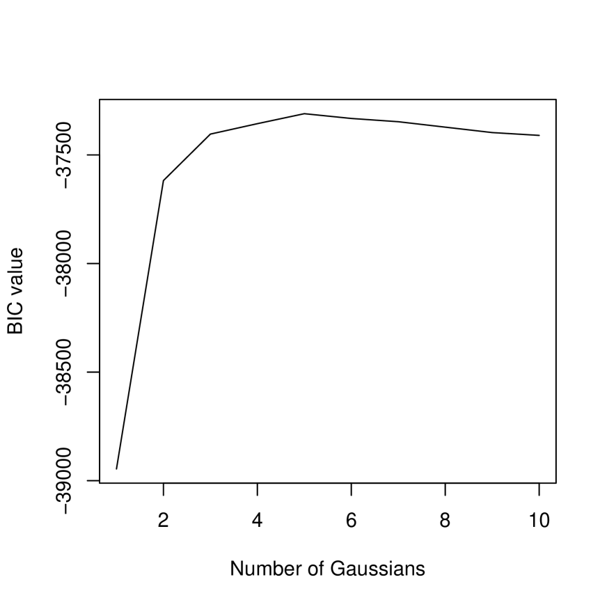
While we have the segmentation of the distance histogram, we need the segmentation of the original financial signal. If we had 2 clusters in the original financial signal, then we could expect up to 3 peaks in the distances histogram (viz., 2 intra-cluster peaks, and 1 inter-cluster peak). If we had 3 clusters in the original financial signal, then we could expect up to 6 peaks in the distances histogram (viz., 3 intra-cluster peaks, and 3 inter-cluster peaks). This information is consistent with asserting that the evidence from Figure 15 points to two of these histogram peaks being approximately co-located (alternatively: the distances are approximately the same). We conclude that 3 clusters in the original financial signal is the most consistent number of clusters. We will now determine these.

One possibility is to use principal coordinates analysis (Torgerson’s, Gower’s metric multidimensional scaling) of the pairwise distances. In fact, a 2-dimensional mapping furnishes a very similar pairwise distance histogram to that seen using the full, 10000, dimensionality. The first axis in Figure 16 accounts for 88.4% of the variance, and the second for 5.8%. Note therefore how the scales of the planar representation in Figure 16 point to it being very linear.

Benzécri (1979, Vol. II, chapter 7, section 3.1) discusses the Guttman effect, or Guttman scale, where factors that are not mutually correlated, are nonetheless functionally related. When there is a “fundamentally unidimensional underlying phenomenon” (there are multiple such cases here) factors are functions of Legendre polynomials. We can view Figure 16 as consisting of multiple horseshoe shapes. A simple explanation for such shapes is in terms of the constraints imposed by lots of equal distances when the data vectors are ordered linearly: see Murtagh (2005, pp. 46-47).

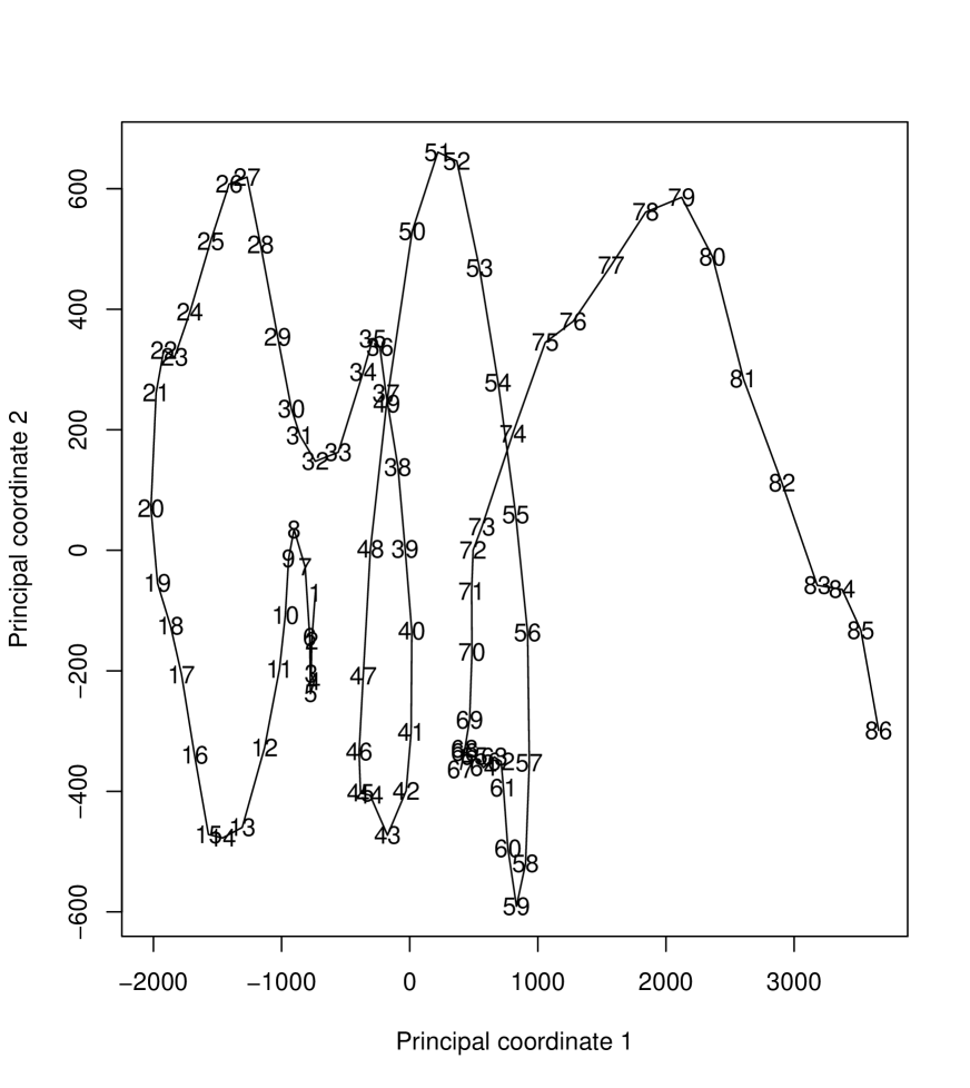
Another view of how embedded (hence clustered) data are capable of being well mapped into a unidimensional curve is Critchley and Heiser (1988). Critchley and Heiser show one approach to mapping an ultrametric into a linearly or totally ordered metric. We have asserted and then established how hierarchy in some form is relevant for high dimensional data spaces; and then we find a very linear projection in Figure 16. As a consequence we note that the Critchley and Heiser result is especially relevant for high dimensional data analysis.

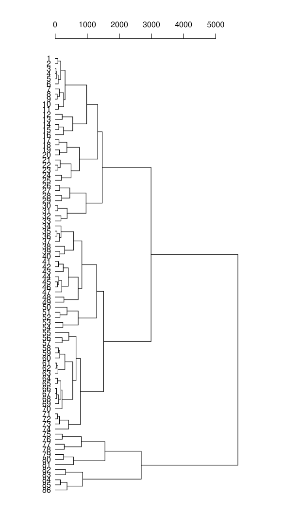
Knowing that 3 clusters in the original signal are wanted, we will use an adjacency-constrained agglomerative hierarchical clustering algorithm to find them: see Figure 17. The contiguity-constrained complete link criterion is our only choice here if we are to be sure that no inversions can come about in the hierarchy, as explained in Murtagh (1985). As input, we use the coordinates in Figure 16. The 2-dimensional Figure 16 representation relates to over 94% of the variance. The most complete basis was of dimensionality 85. We checked the results of the 85-dimensionality embedding which, as noted below, gave very similar results.

Reading off the 3-cluster memberships from Figure 17 gives for the signal actually used (with a very initial segment and a very final segment deleted): cluster 1 corresponds to signal values 1000 to 33999 (points 1 to 33 in Figure 17); cluster 2 corresponds to signal values 34000 to 74999 (points 34 to 74 in Figure 17); and cluster 3 corresponds to signal values 75000 to 86999 (points 75 to 86 in Figure 17). This allows us to segment the original time series: see Figure 18. (The clustering of the 85-dimensional embedding differs minimally. Segments are: points 1 to 32; 33 to 73; and 74 to 86.)

To summarize what has been done:

1.

the segmentation is initially guided by the peak-finding in the histogram of distances
2.

with high dimensionality we expect simple structure in a low dimensional mapping provided by principal coordinates analysis
3.

which we use as input to a sequence-constrained clustering method in order to determine the clusters
4.

which can then be displayed on the original data.

In this case, the clusters are defined using a complete link criterion, implying that these three clusters are determined by minimizing their maximum internal pairwise distance. This provides a strong measure of signal volatility as an explanation for the clusters, in addition to their average value.

5 Conclusions

One interesting conclusion on this work follows. Traditionally, clustering algorithms have generally been considered as distance-based or model-based. The former is exemplified by agglomerative hierarchical clustering, or k-means partitioning. The latter is exemplified by Gaussian mixture modeling. (One motivation for model-based clustering is the computational difficulty, in general, of taking account of all pairwise distances.) The approach described in this work is both distance-based and model-based.

What we have observed in all of this work is that in the limit of high dimensionality a scalar product space becomes ultrametric. It has been our aim in this work to link observed data with an ultrametric topology for such data. The traditional approach in data analysis, of course, is to impose structure on the data. This is done, for example, by using some agglomerative hierarchical clustering algorithm. We can always do this (modulo distance or other ties in the data). Then we can assess the degree of fit of such a (tree or other) structure to our data. For our purposes, here, this is unsatisfactory.

•

Firstly, our aim was to show that ultrametricity can be naturally present in our data, globally or locally. We did not want any “measuring tool” such as an agglomerative hierarchical clustering algorithm to overly influence this finding. (Unfortunately Rammal et al., 1986, suffers from precisely this unhelpful influence of the “measuring tool” of the subdominant ultrametric. In other respects, Rammal et al., 1986, is a seminal paper.)
•

Secondly, let us assume that we did use hierarchical clustering, and then based our discussion around the goodness of fit. This again is a traditional approach used in data analysis, and in statistical data modeling. But such a discussion would have been unnecessary and futile. For, after all, if we have ultrametric properties in our data then many of the widely used hierarchical clustering algorithms will give precisely the same outcome, and furthermore the fit is by definition optimal. (Our point here is that if $\min\{d_{ik}|i\in q,k\not\in q,k\neq q\}=\max\{d_{ik}|i\in q,k\not\in q,k\neq q\}$ for cluster $q$ , at all agglomerations, then single linkage and complete linkage are identical.)

We have described an application of this work to very high frequency signal processing. The twin objectives are signal segmentation, and model identification. We have noted that a considerable amount of this work is model-based: we require assumptions (on clusters, and on model(s)) for identifiability.

Motivation for this work includes the availability of very high frequency data streams in various fields (physics, engineering, finance, meteorology, bio-engineering, and bio-medicine). By using a very large embedding dimensionality, we are approaching the data analysis on a very gross scale, and hence furnishing a particular type of multiresolution analysis. That this is worthwhile has been shown in our case studies.

References

AGGARWAL, C.C., HINNEBURG, A. and KEIM, D.A. (2001). “On the Surprising Behavior of Distance Metrics in High Dimensional Spaces”, Proceedings of the 8th International Conference on Database Theory, pp. 420–434, January 04-06.

AHN, J., MARRON, J.S., MULLER, K.E. and CHI, Y.-Y. (2007). “The High Dimension, Low Sample Size Geometric Representation Holds under Mild Conditions”, Biometrika, 94, 760–766.

AHN, J. and MARRON, J.S. (2005). “Maximal Data Piling in Discrimination”, Biometrika, submitted; and “The Direction of Maximal Data Piling in High Dimensional Space”.

BELLMAN, R. (1961). Adaptive Control Processes: A Guided Tour, Princeton University Press.

BÉNASSÉNI, J., BENNANI DOSSE, M. and JOLY, S. (2007). On a General Transformation Making a Dissimilarity Matrix Euclidean, Journal of Classification, 24, 33–51.

BENZÉCRI, J.P. (1979). L’Analyse des Données, Tome I Taxinomie, Tome II Correspondances, 2nd ed., Dunod, Paris.

BREUEL, T.M. (2007). “A Note on Approximate Nearest Neighbor Methods”, http://arxiv.org/pdf/cs/0703101

CAILLIEZ, F. and PAGÈS, J.P. (1976). Introduction à l’Analyse de Données, SMASH (Société de Mathématiques Appliquées et de Sciences Humaines), Paris.

CAILLIEZ, F. (1983). “The Analytical Solution of the Additive Constant Problem”, Psychometrika, 48, 305–308.

CHÁVEZ, E., NAVARRO, G., BAEZA-YATES, R. and MARROQUÍN, J.L. (2001). “Proximity Searching in Metric Spaces”, ACM Computing Surveys, 33, 273–321.

CRITCHLEY, F. and HEISER, W. (1988), “Hierarchical trees can be perfectly scaled in one dimension” Journal of Classification, 5, 5–20.

DE SOETE, G. (1986). “A Least Squares Algorithm for Fitting an Ultrametric Tree to a Dissimilarity Matrix”, Pattern Recognition Letters, 2, 133–137.

DONOHO, D.L. and TANNER, J. (2005). “Neighborliness of Randomly-Projected Simplices in High Dimensions”, Proceedings of the National Academy of Sciences, 102, 9452–9457.

HALL, P., MARRON, J.S. and NEEMAN, A. (2005). “Geometric Representation of High Dimension Low Sample Size Data”, Journal of the Royal Statistical Society B, 67, 427–444.

HEISER, W.J. (2004). “Geometric Representation of Association between Categories”, Psychometrika, 69, 513–545.

HINNEBURG, A., AGGARWAL, C. and KEIM, D. (2000). “What is the Nearest Neighbor in High Dimensional Spaces?”, VLDB 2000, Proceedings of 26th International Conference on Very Large Data Bases, September 10-14, 2000, Cairo, Egypt, Morgan Kaufmann, pp. 506–515.

HORNIK, K. (2005). “A CLUE for CLUster Ensembles”, Journal of Statistical Software, 14 (12).

KASS, R.E. and RAFTERY, A.E. (1995). “Bayes Factors and Model Uncertainty”, Journal of the American Statistical Association, 90, 773–795.

KHRENNIKOV, A. (1997). Non-Archimedean Analysis: Quantum Paradoxes, Dynamical Systems and Biological Models, Kluwer.

LERMAN, I.C. (1981). Classification et Analyse Ordinale des Données, Paris, Dunod.

MURTAGH, F. (1985). Multidimensional Clustering Algorithms, Physica-Verlag.

MURTAGH, F. (2004). “On Ultrametricity, Data Coding, and Computation”, Journal of Classification, 21, 167–184.

MURTAGH, F. (2005). “Identifying the Ultrametricity of Time Series”, European Physical Journal B, 43, 573–579.

MURTAGH, F. (2007). “A Note on Local Ultrametricity in Text”,
http://arxiv.org/pdf/cs.CL/0701181

MURTAGH, F. (2005). Correspondence Analysis and Data Coding with R and Java, Chapman & Hall/CRC.

MURTAGH, F. (2006). “From Data to the Physics using Ultrametrics: New Results in High Dimensional Data Analysis”, in A.Yu. Khrennikov, Z. Rakić and I.V. Volovich, Eds., p-Adic Mathematical Physics, American Institute of Physics Conf. Proc. Vol. 826, 151–161.

MURTAGH, F., DOWNS, G. and CONTRERAS, P. (2008). “Hierarchical Clustering of Massive, High Dimensional Data Sets by Exploiting Ultrametric Embedding”, SIAM Journal on Scientific Computing, 30, 707–730.

MURTAGH, F. and STARCK, J.L. (2003). “Quantization from Bayes Factors with Application to Multilevel Thresholding”, Pattern Recognition Letters, 24, 2001–2007.

NEUWIRTH, E. and REISINGER, L. (1982). “Dissimilarity and Distance Coefficients in Automation-Supported Thesauri”, Information Systems, 7, 47–52.

RAMMAL, R., ANGLES D’AURIAC, J.C. and DOUCOT, B. (1985). “On the Degree of Ultrametricity”, Le Journal de Physique – Lettres, 46, L-945–L-952.

RAMMAL, R., TOULOUSE, G. and VIRASORO, M.A. (1986). “Ultrametricity for Physicists”, Reviews of Modern Physics, 58, 765–788.

ROHLF, F.J. and FISHER, D.R. (1968). “Tests for Hierarchical Structure in Random Data Sets”, Systematic Zoology, 17, 407–412.

SCHWARZ, G. (1978). “Estimating the Dimension of a Model”, Annals of Statistics, 6, 461–464.

TORGERSON, W.S. (1958). Theory and Methods of Scaling, Wiley.

TREVES, A. (1997). “On the Perceptual Structure of Face Space”, BioSystems, 40, 189–196.