Accelerated kinetic Monte Carlo algorithm for diffusion limited kinetics

Abstract

If a stochastic system during some periods of its evolution can be divided into non-interacting parts, the kinetics of each part can be simulated independently. We show that this can be used in the development of efficient Monte Carlo algorithms. As an illustrative example the simulation of irreversible growth of extended one dimensional islands is considered. The new approach allowed to simulate the systems characterized by parameters superior to those used in previous simulations.

A unique feature of the kinetic Monte Carlo (kMC) technique which to a large extent underlies its wide acceptance in physics is its ability to provide essentially exact data describing complex far-from-equilibrium phenomena binder . The technique, however, is rather demanding on computational resources which in many cases makes the simulations either impractical or altogether impossible ratsch-venables-review ; no-scaling . As was pointed out in Ref. ratsch-venables-review , the major cause of the low efficiency of kMC is the large disparity between the time scales of the participating processes. In fact, it is the fastest process which slows down the simulation the most. As a remedy it was suggested that the fast processes were described in some averaged, mean-field manner. These and similar observations lie at the hart of various approximate multi-scale schemes (see, e. g., Refs. ratsch-venables-review ; multiscalePRL ; 1Dmultiscale ; 2Dmultiscale ; 3Dmultiscale ).

The approximate implementations, however, deprive kMC of its major asset—the exactness. As a consequence, it cannot serve as a reliable tool for resolving controversial issues, such, e. g., as those arising in connection with the scaling laws governing the irreversible epitaxial growth (see Refs. no-scaling ; 1Dmultiscale ; famarescu and references therein).

Recently, an exact kMC scheme called by the authors the first-passage algorithm (FPA) was proposed which avoids simulating all the hops of freely diffusing atoms and using instead analytic solutions of an appropriate diffusion equation FPT_MC . It is premature yet draw definite conclusions about the efficiency of the algorithm tested only on one system, at least before additional technical issues improving its efficiency are published by the authors. However, the authors themselves note that there are problems in the treatment of closely spaced atoms. This makes it difficult to use FPA in simulating the diffusion limited kinetics in such cases when along with large empty spaces where the analytic description is efficient there exist the reaction zones where the particle concentrations are high as, e. g., in the vicinity of islands during the surface growth. Furthermore, because the majority of kMC simulations are performed with the use of the by now classic event-based algorithm (EBA) of Ref. n-fold , the FPA algorithm would be difficult to use in the upgrade of the existing code. This is because FPA is completely different from EBA and its application would require a new code to be created from the scratch. In some cases this may be more time-consuming than the use of the available EBA code.

The aim of the present paper is to propose an exact accelerated kMC algorithm which extends the EBA in such a way that in the case of the diffusion limited systems only the atoms which are sufficiently well separated from the reaction zones are treated with the use of exact diffusion equations while in the high-density regions the conventional EBA is used.

The algorithm we are going to present can be applied to any separable model. For concreteness, we present it using as an example a simple (but non-trivial—see amar_popescu and references therein) example of the irreversible growth in one dimension (1d) 1992 ; 1Dscaling ; amar_popescu . Its generalizations to other systems are completely straightforward,

Our approach is based on the observation that the fastest process in the surface growth is the hopping diffusion of the isolated atoms (or monomers) ratsch-venables-review . Random walk on a lattice is one of the best studied stochastic phenomena with a lot of exact information available. In cases when the monomers are well separated from each other and from the growth regions, the analytical description of their diffusion can be computationally much less demanding than straightforward kMC simulation.

In the model of irreversible growth the atoms are deposited on the surface at rate $F$ where they freely diffuse until meeting either another atom or an island edge which results either in the nucleation of a new island or in the growth of an existing one, respectively. To illustrate the strength of our approach, we will study the limit of low coverages $\theta\to 0$ because in Ref. no-scaling this limit was considered to be difficult to simulate in the case of extended islands. Because the scaling limit corresponds to

$$R\equiv D/F\to\infty,$$ (1)

(where $D$ is the diffusion constant) i. e., to very low deposition rates, and, furthermore, because the covered regions are also small due to low $\theta$, we found it reasonable to neglect nucleation on the tops of islands by assuming them to be monolayer-high.

In its simplest implementation our algorithm is based on a subdivision of the monomers into two groups (A and B) which at a given moment are considered to be active (A) and passive (B) ones with respect to the growth processes. The passive monomers are those which are too far away from the places of attachment to existing islands or of nucleation of new ones. This can be quantified with the use of a separation length $L$. Thus, an atom is considered to be passive if it is separated from a nearest island by more then $L$ sites or if its separation from a nearest monomer exceeds $2L$. The monomers which do not satisfy these restrictions are considered to be actively participating in the growth and thus belonging to the group A. It is the passive atoms B that we are going to treat within an analytical approach instead of simulating them via kMC. Thus, in contrast to FPA where all atoms should be boxed, in our algorithm we may box only those which will spend some appreciable time inside the boxes and will not need to be quickly re-boxed as in the FPA algorithm with closely spaced atoms.

Formally this is done as follows. Let us place all B atoms in the middle of 1d “boxes” of length $L_{\mbox{Box}}=2L+1$. Assuming the central site has the coordinate $i=0$, the initial probability distribution is of the Kronecker delta form

$$p(i,t=0)=\delta_{i0},$$ (2)

where the time variable $t$ counts the time spent by the atom inside the box. With the atomic hopping rate set to unity, the evolution of the probability distribution of an atom inside the box satisfies the equations

$$\frac{\partial p(i,t)}{\partial t} = \frac{1}{2}p(i+1,t)+\frac{1}{2}p(i-1,t)-p(i,t)$$ (3a)

$$\frac{\partial p(\pm L,t)}{\partial t} = \frac{1}{2}p(\pm(L-1),t)-\frac{1}{2}p(\pm L,t),$$ (3b)

where $|i|<L$. The first equation expresses the conservation of probability on the interior sites $i\not=\pm L$. The change of probability on site $i$ given by the time derivative on the left hand side comes from the probability of atoms hopping from neighbor sites $i\pm 1$ (two positive terms on the right hand side) minus the probability for the atom to escape the site. The “in” terms have weights 1/2 because the atoms have two equivalent directions to hop. The boundary equations (3b) differ only in that there are neither incoming flux from the outside of the box, nor the outgoing flux in this direction.

The solution at an arbitrary time can be written as

$$p(i,t)=L_{\mbox{Box}}^{-1}\left[1+2\sum_{m=1}^{L}e^{-\epsilon_{m}t}\cos(\alpha mi)\right],$$ (4)

where

$$\alpha=2\pi/L_{\mbox{Box}}\qquad\mbox{and}\qquad\epsilon_{m}=2\sin^{2}(\alpha m/2).$$ (5)

The distribution Eq. (4) satisfies Eqs. (3) as can be checked by direct substitution. The initial condition Eq. (2) as well as the probability conservation $\sum_{i}p(i,t)=1$ can be verified with the use of Eq. 1.342.2 from Ref. GR . In our algorithm we will need to repeatedly calculate $p(i,t)$, so its efficient calculation is important. Eq. (4) is formally a discrete Fourier transform, so it is natural to use an FFT algorithm. Because our choice for the position of the atom in the center of the box makes the box length odd ($L_{\mbox{Box}}=2L+1$), we used the radix-3 algorithm of Ref. FFT , so the sizes of all our boxes below are powers of 3.

The gain in the speed of the simulation is achieved because as long as atoms B stay within the boxes we do not waste computational resources to simulate them by knowing that they evolve according to Eq. (4).

Obviously, sooner or later the atomic configuration will change so that the A-B division will cease to be valid. This happens, in particular, when an atom leaves the box. Because the hopping in the model is allowed only at the nearest neighbor (NN) distance, only the atoms at sites $\pm L$ may leave the box. With the hopping probability being 1/2 at each side, the probability of an atom to leave the box is

$$P_{\mbox{end}}(t)\equiv p(\pm L,t).$$ (6)

By repeated differentiation of (6) with the use of Eqs. (3) it can be shown that as $t\to 0$ $P_{\mbox{end}}(t)=O(t^{L})$ which means that for sufficiently large boxes the probability is very close to zero at small $t$. From the graph of this function plotted on Fig. 1 it is seen that the probability of leaving the box is practically zero for $t\lesssim 0.02L_{\mbox{Box}}^{2}$.

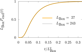
Figure 1: (Color online) Time-dependent probability rate $P_{\mbox{end}}(t)$ for the boxed atom to escape from the box.

Let us consider a 1d “surface” consisting of $K$ cites with the cyclic boundary conditions being imposed (site $i=K$ being identical to site $i=0$). Let the configuration at time $t$ consists of $n_{A}$ active atoms, $n_{B}$ boxed atoms, and $n$ islands. This configuration will change with the time-dependent rate (cf. Ref. n-fold where the only difference is that the rate is constant)

$$\lambda(t)=FK+n_{A}+n_{B}P_{\mbox{end}}(t),$$ (7)

where the first term describes the rate of deposition of new atoms, the second corresponds to a hop of an active atom A to a NN site (we remind that the hopping rate is set to unity) and the last term describes the rate of B atoms getting out of the boxes. Because the rate is time-dependent, we are faced with the necessity to simulate the nonhomogeneous Poisson process (the EBA is the homogeneous Poisson process). We will do this by using the thinning method thinning in its simplest realization with a constant auxiliary rate $\lambda^{*}$ satisfying

$$\lambda^{*}\geq\lambda(t).$$ (8)

We chose it as

$$\lambda^{*}=FK+n_{A}+n_{B}/L_{\mbox{Box}}.$$ (9)

From Fig. 1 it is seen that Eq. (8) is satisfied.

In its most straightforward realization our algorithm consists in the following steps.
1. Generate a random uniform variate $u\in(0,1]$ and advance the time in the boxes as

$$t\to t-\ln(u)/\lambda^{*};$$ (10)

2. Generate another $u$, calculate the rate $\bar{\lambda}=u\lambda^{*}$, and check whether the inequality

$$\bar{\lambda}\leq\lambda(t)$$ (11)

holds. If not, loop back to step 1; if yes go to the next step;
3a. If $\bar{\lambda}\leq FK$ the deposition event takes place. Chose randomly the deposition site and go to step 4;
3b. $FK<\bar{\lambda}\leq FK+n_{A}$ corresponds to the atomic jump. Move a randomly chosen atom to one of NN sites and if this site is a neighbor to a box or to another atom go to step 4; otherwise loop back to step 1, diminishing $n_{A}$ by one if the jump site was a NN site of an island, so that the atom gets attached to it;
3c. Finally, if $FK+n_{A}<\bar{\lambda}\leq\lambda(t)$, an atom leaves the box; chose at random the box and the exit side; go to the next step;
4. Calculate $\exp(-\epsilon_{m}t)$ using Eq. (5) and find the probability distribution via the FFT in Eq. (4). For each boxed atom generate a discrete random variable $-L\leq i\leq L$ with the distribution $p(i,t)$ and place the atom previously in the box centered at $i_{B}$ at site $(i_{B}+i\mod K)$. Then depending on step 3 nucleate a new island or add the deposited atom at the random site chosen. If the site turns out to be on top of an island move it to the nearest edge, chose it at random if exactly in the middle. In this way we avoid the nucleation on tops of islands. This prescription is not unique and can be replaced if necessary;
5. Separate the atoms into groups A and B; reset the time inside boxes to zero ($t=0$); loop back to step 1.

The majority of the above steps were chosen mainly for their simplicity with no serious optimization attempted. In the simulations below the performance was optimized only through the choice of the box size $L_{\mbox{Box}}$ which was the same throughout the simulation, though it seems obvious that by choosing different $L_{\mbox{Box}}$ at different stages of growth should improve the performance because of the density which changes with time. Leaving this and similar improvements for future studies, in the present paper we checked the central point of the algorithm which consists in its step 2. Because with an appropriate choice of $L_{\mbox{Box}}$ most of the atoms are boxed (up to 100% at the early stage) and because the deposition rate $F$ is very small [see Eq. (1)], at small $t$ the simulation makes a lot of cycles between the 1st and the 2nd steps due to the small acceptance ratio (see Fig. 1). Thus, by simply generating the random variates we simulate diffusion of all boxed atoms.

We simulated the model with the parameters shown in Figs. 2–4 with $K$ (the system size) in the range $10^{6}$–$10^{7}$ on a 180 MHz MIPS processor. Our primary goal was to validate our kMC algorithm and to check the possibility to extend the parameter ranges achieved in previous studies. To the best of our knowledge, we succeeded in carrying over the simulations with the values of major parameters, such as $R$ and $K$ exceeding those in previous studies while our smallest value of coverage is the smallest among those used previously in kMC simulations. This was achieved with the maximum execution time (for one run) slightly larger than 2.5 h. We expect that with better optimization with modern processors even better results can be achieved.

Though no systematic study of scaling was attempted, the data on the scaling function $f$ defined as 1992

$$N_{s}=\frac{\theta}{S^{2}}f\left(\frac{s}{S}\right)$$ (12)

(where $N_{s}$ is the density of islands of size $s$ and $S=\sum_{s=2}^{\infty}sN_{s}$ is the mean island size) presented on Fig. 3 show perfect scaling for all tree cases studied which differ 6 orders of magnitude in the deposition rate and two orders of magnitude in coverage. No dependence of $f(0)$ on $\theta$ found in Ref. famarescu is seen in our Fig. 3 though the range of variation of $\theta$ is more than two orders of magnitude larger. The index $z=3/4$ used in Fig. 4 to fit the data on $N\equiv n/K$ provides better fit then the value $z=1$ suggested in Ref. famarescu for the extended islands. In our opinion, the point island value is a reasonable choice at very low coverages because the island sizes became negligible in comparison with the interisland separations (the gap sizes). The situation needs further investigation because another index $r$ was found to be equal to $\sim 0.64$ while the mean field theory predicts it to be 1/2 1992 ; 1Dscaling . Presumably, the value of $R=5\times 10^{9}$ used by us was not sufficiently large for the scaling to set in. We note, however, that it is 500 times larger than that used in Ref. famarescu .

Figure 2: Illustration of independence of the island size distribution on the length of the box $L_{\mbox{Box}}$ used in the simulation algorithm; from 90 to 100% of atoms were boxed for $L_{\mbox{Box}}=9$ and from 90 to 100% were not boxed for $L_{\mbox{Box}}=2187$ (for further explanations see the text). The same statistics corresponding to $10^{6}$ deposited atoms was gathered for each box size.

Figure 3: The scaled island size distribution function defined in Eq. (12) as obtained in the kMC simulations explained in the text. The optimum box sizes were 81, 243, and 729 for $\theta=0.1$, 0.01, and 0.001, respectively. Statistics of $5\times 10^{5}$ atoms was gathered in each of the three cases studied. Because of the scaling law $S\propto\theta^{3/4}R^{1/4}$ 1Dscaling the number of islands simulated in all three cases was approximately the same.

Figure 4: Island ($N$) and monomer ($N_{1}$) densities at different coverages. The dashed line describes the fit to the asymptotics $N\propto\theta^{1-z}$ with $z=3/4$ 1992 ; 1Dscaling ; the dashed-dotted line is the fit to the asymptotics $N_{1}\propto\theta^{-r}$ with $r\approx 0.64$.

In conclusion we would like to stress that the technique presented above can be applied to any separable systems, not only to case considered in the present paper. Neither the availability of an analytical solution is critical. The solution for the subsystems can be numerical or even obtained via kMC simulations. Further modifications may include introduction of several scales, e. g., with the use of the boxes of different sizes as in Ref. FPT_MC ; the subsystems chosen can be different at different stages of the simulation. In brief, we believe that the technique proposed is sufficiently flexible to allow for the development of efficient kMC algorithms for broad class of separable systems.

- (1) K. Binder, in Monte Carlo Methods in Statistical Physics, edited by K. Binder (Springer-Verlag, Heidelberg, 1986), vol. 7 of Topics in Current Physics, p. 1.
- (2) C. Ratsch and J. A. Venables, J. Vac. Sci. Technol. A 21, S96 (2003).
- (3) C. Ratsch, Y. Landa, and R. Vardavas, Surface Science 578, 196 (2005).
- (4) C. A. Haselwandter and D. D. Vvedensky, Phys. Rev. Lett. 98, 046102 (2007).
- (5) C.-C. Chou and M. L. Falk, J. of Comput. Phys. 217, 519 (2006).
- (6) J. P. DeVita, L. M. Sander, and P. Smereka, Physical Review B 72, 205421 (2005).
- (7) C.-C. Fu, J. Dalla Torre, F. Willaime, J.-L. Bocquet, and A. Barbu, Nat. Mater. 4, 68 (2005).
- (8) J. G. Amar, M. N. Popescu, and F. Family, Surf. Sci. 491, 239 (2001).
- (9) T. Opplestrup, V. V. Bulatov, G. H. Gilmer, M. H. Kalos, and B. Sadigh, Phys. Rev. Lett. 97, 230602 (2006).
- (10) A. B. Bortz, M. H. Kalos, and J. L. Lebowitz, J. Comput. Phys. 17, 10 (1975).
- (11) J. G. Amar and M. N. Popescu, Phys. Rev. B 69, 033401 (2004).
- (12) M. C. Bartelt and J. W. Evans, Phys. Rev. B 46, 12675 (1992).
- (13) J. A. Blackman and P. A. Mulheran, Phys. Rev. B 54, 11681 (1996).
- (14) I. S. Gradshtein and I. M. Ryzhik, Tables of Integrals Series and Products (Academic Press, New York, 1965).
- (15) D. Takahashi and Y. Kanada, J. Supercomputing 15, 207 (2000).
- (16) P. A. W. Lewis and G. S. Shedler, Naval Res. Logist. Quart. 26, 403 (1979).