Symmetry in Data Mining and Analysis: A Unifying View Based on Hierarchy

Abstract

Data analysis and data mining are concerned with unsupervised pattern finding and structure determination in data sets. The data sets themselves are explicitly linked as a form of representation to an observational or otherwise empirical domain of interest. “Structure” has long been understood as symmetry which can take many forms with respect to any transformation, including point, translational, rotational, and many others. Symmetries directly point to invariants, that pinpoint intrinsic properties of the data and of the background empirical domain of interest. As our data models change so too do our perspectives on analyzing data. The structures in data surveyed here are based on hierarchy, represented as p-adic numbers or an ultrametric topology.

Keywords: Data analytics, multivariate data analysis, pattern recognition, information storage and retrieval, clustering, hierarchy, p-adic, ultrametric topology, complexity

1 Introduction

Herbert A. Simon, Nobel Laureate in Economics, originator of “bounded rationality” and of “satisficing”, believed in hierarchy at the basis of the human and social sciences, as the following quotation shows: “… my central theme is that complexity frequently takes the form of hierarchy and that hierarchic systems have some common properties independent of their specific content. Hierarchy, I shall argue, is one of the central structural schemes that the architect of complexity uses.” ([74], p. 184.)

Partitioning a set of observations [76, 77, 53] leads to some very simple symmetries. This is one approach to clustering and data mining. But such approaches, often based on optimization, are really not of direct interest to us here. Instead we will pursue the theme pointed to by Simon, namely that the notion of hierarchy is fundamental for interpreting data and the complex reality which the data expresses. Our work is very different too from the marvelous view of the development of mathematical group theory – but viewed in its own right as a complex, evolving system – presented by Foote [20].

1.1 Structure in Observed or Measured Data

Weyl [83] makes the case for the fundamental importance of symmetry in science, engineering, architecture, art and other areas. As a “guiding principle”, “Whenever you have to do with a structure-endowed entity … try to determine its group of automorphisms, the group of those element-wise transformations which leave all structural relations undisturbed. You can expect to gain a deep insight in the constitution of [the structure-endowed entity] in this way. After that you may start to investigate symmetric configurations of elements, i.e. configurations which are invariant under a certain subgroup of the group of all automorphisms; …” ([83], p. 144).

“Symmetry is a vast subject, significant in art and nature.”, Weyl states (p. 145), and no better example of the “mathematical intellect” at work. “Although the mathematics of group theory and the physics of symmetries were not fully developed simultaneously – as in the case of calculus and mechanics by Newton – the intimate relationship between the two was fully realized and clearly formulated by Wigner and Weyl, among others, before 1930.” ([78], p. 1.) Powerful impetus was given to this (mathematical) group view of study and exploration of symmetry in art and nature by Felix Klein’s 1872 Erlangen Program [41] which proposed that geometry was at heart group theory: geometry is the study of groups of transformations, and their invariants. Klein’s Erlangen Program is at the cross-roads of mathematics and physics. The purpose of this article is to locate symmetry and group theory at the cross-roads of data mining and data analytics too.

1.2 About this Article

In section 2, we describe ultrametric topology as an expression of hierarchy.

In section 3, p-adic encoding, providing a number theory vantage point on ultrametric toplogy, gives rise to additional symmetries and ways to capture invariants in data.

Section 4 deals with symmetries that are part and parcel of a tree, representing a partial order on data, or equally a set of subsets of the data, some of which are embedded.

In section 5 permutations are at issue, including permutations that have the property of representing hierarchy.

Section 6 deals with new and recent results relating to the remarkable symmetries of massive, and especially high dimensional data sets.

1.3 A Brief Introduction to Hierarchical Clustering

For the reader new to analysis of data a very short introduction is now provided on hierarchical clustering. Along with other families of algorithm, the objective is automatic classification, for the purposes of data mining, or knowledge discovery. Classification, after all, is fundamental in human thinking, and machine-based decision making. But we draw attention to the fact that our objective is unsupervised, as opposed to supervised classification, also known as discriminant analysis or (in a general way) machine learning. So here we are not concerned with generalizing the decision making capability of training data, nor are we concerned with fitting statistical models to data so that these models can play a role in generalizing and predicting. Instead we are concerned with having “data speak for themselves”. That this unsupervised objective of classifying data (observations, objects, events, phenomena, etc.) is a huge task in our society is unquestionably true. One may think of situations when precedents are very limited, for instance.

Among families of clustering, or unsupervised classification, algorithms, we can distinguish the following: (i) array permuting and other visualization approaches; (ii) partitioning to form (discrete or overlapping) clusters through optimization, including graph-based approaches; and – of interest to us in this article – (iii) embedded clusters interrelated in a tree-based way.

For the last-mentioned family of algorithm, agglomerative building of the hierarchy from consideration of object pairwise distances has been the most common approach adopted. As comprehensive background texts, see [52, 29, 84, 30].

1.4 A Brief Introduction to p-Adic Numbers

The real number system, and a p-adic number system for given prime, p, are potentially equally useful alternatives. p-Adic numbers were introduced by Kurt Hensel in 1898.

Whether we deal with Euclidean or with non-Euclidean geometry, we are (nearly) always dealing with reals. But the reals start with the natural numbers, and from associating observational facts and details with such numbers we begin the process of measurement. From the natural numbers, we proceed to the rationals, allowing fractions to be taken into consideration.

The following view of how we do science or carry out other quantitative study was proposed by Volovich in 1987 [80, 81]. See also Freund [23]. We can always use rationals to make measurements. But they will be approximate, in general. It is better therefore to allow for observables being “continuous, i.e. endow them with a topology”. Therefore we need a completion of the field $\mathbb{Q}$ of rationals. To complete the field $\mathbb{Q}$ of rationals, we need Cauchy sequences and this requires a norm on $\mathbb{Q}$ (because the Cauchy sequence must converge, and a norm is the tool used to show this). There is the Archimedean norm such that: for any $x,y\in\mathbb{Q}$, with $|x|<|y|$, then there exists an integer $N$ such that $|Nx|>|y|$. For convenience here, we write: $|x|_{\infty}$ for this norm. So if this completion is Archimedean, then we have $\mathbb{R}=\mathbb{Q}_{\infty}$, the reals. That is fine if space is taken as commutative and Euclidean.

What of alternatives? Remarkably all norms are known. Besides the $\mathbb{Q}_{\infty}$ norm, we have an infinity of norms, $|x|_{p}$, labeled by primes, p. By Ostrowski’s theorem [66] these are all the possible norms on $\mathbb{Q}$. So we have an unambiguous labeling, via p, of the infinite set of non-Archimedean completions of $\mathbb{Q}$ to a field endowed with a topology.

In all cases, we obtain locally compact completions, $\mathbb{Q}_{p}$, of $\mathbb{Q}$. They are the fields of p-adic numbers. All these $\mathbb{Q}_{p}$ are continua. Being locally compact, they have additive and multiplicative Haar measures. As such we can integrate over them, such as for the reals.

1.5 Brief Discussion of p-Adic and m-Adic Numbers

We will use p to denote a prime, and m to denote a non-zero positive integer. A p-adic number is such that any set of p integers which are in distinct residue classes modulo p may be used as p-adic digits. (Cf. remark below, at the end of section 3.1, quoting from [26]. It makes the point that this opens up a range of alternative notation options in practice.) Recall that a ring does not allow division, while a field does. m-Adic numbers form a ring; but p-adic numbers form a field. So a priori, 10-adic numbers form a ring. This provides us with a reason for preferring p-adic over m-adic numbers.

We can consider various p-adic expansions:

1. $\sum_{i=0}^{n}a_{i}p^{i}$, which defines positive integers. For a p-adic number, we require $a_{i}\in{0,1,...p-1}$. (In practice: just write the integer in binary form.)

2. $\sum_{i=-\infty}^{n}a_{i}p^{i}$ defines rationals.

3. $\sum_{i=k}^{\infty}a_{i}p^{i}$ where $k$ is an integer, not necessarily positive, defines the field $\mathbb{Q}_{p}$ of p-adic numbers.

$\mathbb{Q}_{p}$, the field of p-adic numbers, is (as seen in these definitions) the field of p-adic expansions.

The choice of p is a practical issue. Indeed, adelic numbers use all possible values of p (see [9] for extensive use and discussion of the adelic number framework). Consider [17, 40]. DNA (desoxyribonucleic acid) is encoded using four nucleotides: A, adenine; G, guanine; C, cytosine; and T, thymine. In RNA (ribonucleic acid) T is replaced by U, uracil. In [17] a 5-adic encoding is used, since 5 is a prime and thereby offers uniqueness. In [40] a 4-adic encoding is used, and a 2-adic encoding, with the latter based on 2-digit boolean expressions for the four nucleotides (00, 01, 10, 11). A default norm is used, based on a longest common prefix – with p-adic digits from the start or left of the sequence (see section 3.2 below where this longest common prefix norm or distance is used).

2 Ultrametric Topology

In this section we mainly explore symmetries related to: geometric shape; matrix structure; and lattice structures.

2.1 Ultrametric Space for Representing Hierarchy

Consider Figure 1, illustrating the ultrametric distance and its role in defining a hierarchy. An early, influential paper is Johnson [34] and an important survey is that of Rammal et al. [68]. Discussion of how a hierarchy expresses the semantics of change and distinction can be found in [63].

The ultrametric topology was introduced by Marc Krasner [44], the ultrametric inequality having been formulated by Hausdorff in 1934. Essential motivation for the study of this area is provided by [71] as follows. Real and complex fields gave rise to the idea of studying any field $K$ with a complete valuation $|.|$ comparable to the absolute value function. Such fields satisfy the “strong triangle inequality” $|x+y|\leq\mbox{max}(|x|,|y|)$. Given a valued field, defining a totally ordered Abelian (i.e. commutative) group, an ultrametric space is induced through $|x-y|=d(x,y)$. Various terms are used interchangeably for analysis in and over such fields such as p-adic, ultrametric, non-Archimedean, and isosceles. The natural geometric ordering of metric valuations is on the real line, whereas in the ultrametric case the natural ordering is a hierarchical tree.

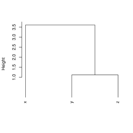
Figure 1: The strong triangular inequality defines an ultrametric: every triplet of points satisfies the relationship: $d(x,z)\leq\mbox{max}\{d(x,y),d(y,z)\}$ for distance $d$. Cf. by reading off the hierarchy, how this is verified for all $x,y,z$: $d(x,z)=3.5;d(x,y)=3.5;d(y,z)=1.0$. In addition the symmetry and positive definiteness conditions hold for any pair of points.

2.2 Some Geometrical Properties of Ultrametric Spaces

We see from the following, based on [46] (chapter 0, part IV), that an ultrametric space is quite different from a metric one. In an ultrametric space everything “lives” on a tree.

In an ultrametric space, all triangles are either isosceles with small base, or equilateral. We have here very clear symmetries of shape in an ultrametric topology. These symmetry “patterns” can be used to fingerprint data data sets and time series: see [59, 60] for many examples of this.

Some further properties that are studied in [46] are: (i) Every point of a circle in an ultrametric space is a center of the circle. (ii) In an ultrametric topology, every ball is both open and closed (termed clopen). (iii) An ultrametric space is 0-dimensional (see [10, 70]). It is clear that an ultrametric topology is very different from our intuitive, or Euclidean, notions. The most important point to keep in mind is that in an ultrametric space everything “lives” in a hierarchy expressed by a tree.

2.3 Ultrametric Matrices and Their Properties

For an $n\times n$ matrix of positive reals, symmetric with respect to the principal diagonal, to be a matrix of distances associated with an ultrametric distance on $X$, a sufficient and necessary condition is that a permutation of rows and columns satisfies the following form of the matrix:

1. Above the diagonal term, equal to 0, the elements of the same row are non-decreasing.

2. For every index $k$, if

   $$d(k,k+1)=d(k,k+2)=\dots=d(k,k+\ell+1)$$

   then

   $$d(k+1,j)\leq d(k,j)\mbox{ for }k+1<j\leq k+\ell+1$$

   and

   $$d(k+1,j)=d(k,j)\mbox{ for }j>k+\ell+1$$

   Under these circumstances, $\ell\geq 0$ is the length of the section beginning, beyond the principal diagonal, the interval of columns of equal terms in row $k$.

To illustrate the ultrametric matrix format, consider the small data set shown in Table 1. A dendrogram produced from this is in Figure 2. The ultrametric matrix that can be read off this dendrogram is shown in Table 2. Finally a visualization of this matrix, illustrating the ultrametric matrix properties discussed above, is in Figure 3.

	Sepal.Length	Sepal.Width	Petal.Length	Petal.Width
iris1	5.1	3.5	1.4	0.2
iris2	4.9	3.0	1.4	0.2
iris3	4.7	3.2	1.3	0.2
iris4	4.6	3.1	1.5	0.2
iris5	5.0	3.6	1.4	0.2
iris6	5.4	3.9	1.7	0.4
iris7	4.6	3.4	1.4	0.3

Table 1: Input data: 8 iris flowers characterized by sepal and petal widths and lengths. From Fisher’s iris data [18].

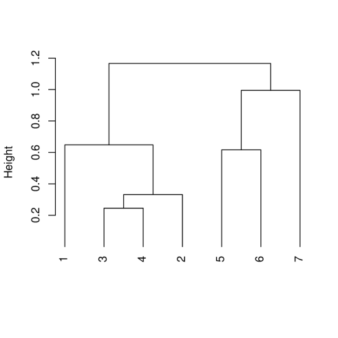
Figure 2: Hierarchical clustering of 7 iris flowers using data from Table 1. No data normalization was used. The agglomerative clustering criterion was the minimum variance or Ward one.

	iris1	iris2	iris3	iris4	iris5	iris6	iris7
iris1	0	0.6480741	0.6480741	0.6480741	1.1661904	1.1661904	1.1661904
iris2	0.6480741	0	0.3316625	0.3316625	1.1661904	1.1661904	1.1661904
iris3	0.6480741	0.3316625	0	0.2449490	1.1661904	1.1661904	1.1661904
iris4	0.6480741	0.3316625	0.2449490	0	1.1661904	1.1661904	1.1661904
iris5	1.1661904	1.1661904	1.1661904	1.1661904	0	0.6164414	0.9949874
iris6	1.1661904	1.1661904	1.1661904	1.1661904	0.6164414	0	0.9949874
iris7	1.1661904	1.1661904	1.1661904	1.1661904	0.9949874	0.9949874	0

Table 2: Ultrametric matrix derived from the dendrogram in Figure 2.

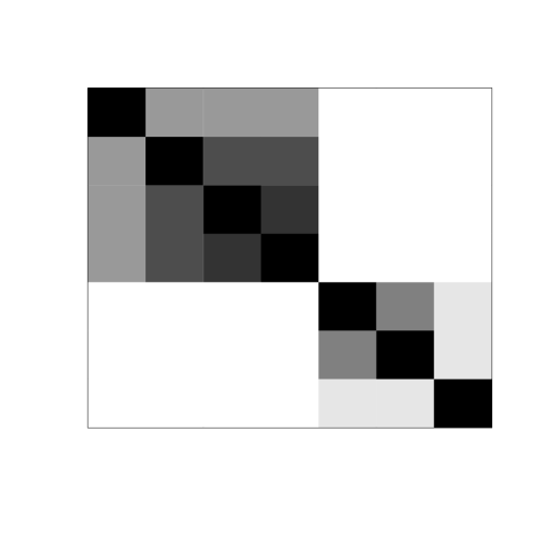
Figure 3: A visualization of the ultrametric matrix of Table 2, where bright or white = highest value, and black = lowest value.

2.4 Clustering Through Matrix Row and Column Permutation

Figure 3 shows how an ultrametric distance allows a certain structure to be visible (quite possibly, in practice, subject to an appropriate row and column permuting), in a matrix defined from the set of all distances. For set $X$, then, this matrix expresses the distance mapping of the Cartesian product, $d:X\times X\longrightarrow\mathbb{R}^{+}$. $\mathbb{R}^{+}$ denotes the non-negative reals. A priori the rows and columns of the function of the Cartesian product set $X$ with itself could be in any order. The ultrametric matrix properties establish what is possible when the distance is an ultrametric one. Because the matrix (a 2-way data object) involves one mode (due to set $X$ being crossed with itself; as opposed to the 2-mode case where an observation set is crossed by an attribute set) it is clear that both rows and columns can be permuted to yield the same order on $X$. A property of the form of the matrix is that small values are at or near the principal diagonal.

A generalization opens up for this sort of clustering by visualization scheme. Firstly, we can directly apply row and column permuting to 2-mode data, i.e. to the rows and columns of a matrix crossing indices $I$ by attributes $J$, $a:I\times J\longrightarrow\mathbb{R}$. A matrix of values, $a(i,j)$, is furnished by the function $a$ acting on the sets $I$ and $J$. Here, each such term is real-valued. We can also generalize the principle of permuting such that small values are on or near the principal diagonal to instead allow similar values to be near one another, and thereby to facilitate visualization. An optimized way to do this was pursued in [50, 49]. Comprehensive surveys of clustering algorithms in this area, including objective functions, visualization schemes, optimization approaches, presence of constraints, and applications, can be found in [51, 48]. See too [15, 57].

For all these approaches, underpinning them are row and column permutations, that can be expressed in terms of the permutation group, $S_{n}$, on $n$ elements.

2.5 Other Miscellaneous Symmetries

As examples of various other local symmetries worthy of consideration in data sets consider subsets of data comprising clusters, and reciprocal nearest neighbor pairs.

Given an observation set, $X$, we define dissimilarities as the mapping $d:X\times X\longrightarrow\mathbb{R}^{+}$. A dissimilarity is a positive, definite, symmetric measure (i.e., $d(x,y)\geq 0;d(x,y)=0\mbox{ if }x=y;d(x,y)=d(y,x)$). If in addition the triangular inequality is satisfied (i.e., $d(x,y)\leq d(x,z)+d(z,y),\forall x,y,z\in X$) then the dissimilarity is a distance.

If $X$ is endowed with a metric, then this metric is mapped onto an ultrametric. In practice, there is no need for $X$ to be endowed with a metric. Instead a dissimilarity is satisfactory.

A hierarchy, $H$, is defined as a binary, rooted, node-ranked tree, also termed a dendrogram [7, 34, 46, 57]. A hierarchy defines a set of embedded subsets of a given set of objects $X$, indexed by the set $I$. That is to say, object $i$ in the object set $X$ is denoted $x_{i}$, and $i\in I$. These subsets are totally ordered by an index function $\nu$, which is a stronger condition than the partial order required by the subset relation. The index function $\nu$ is represented by the ordinate in Figure 2 (the “height” or “level”). A bijection exists between a hierarchy and an ultrametric space.

Often in this article we will refer interchangeably to the object set, $X$, and the associated set of indices, $I$.

Usually a constructive approach is used to induce $H$ on a set $I$. The most efficient algorithms are based on nearest neighbor chains, which by definition end in a pair of agglomerable reciprocal nearest neighbors. Further information can be found in [54, 55, 57, 58].

2.6 Generalized Ultrametric

In this subsection, we consider an ultrametric defined on the power set or join semilattice. Comprehensive background on ordered sets and lattices can be found in [13]. A review of generalized distances and ultrametrics can be found in [72].

2.6.1 Link with Formal Concept Analysis

Typically hierarchical clustering is based on a distance (which can be relaxed often to a dissimilarity, not respecting the triangular inequality, and mutatis mutandis to a similarity), defined on all pairs of the object set: $d:X\times X\rightarrow\mathbb{R}^{+}$. I.e., a distance is a positive real value. Usually we require that a distance cannot be 0-valued unless the objects are identical. That is the traditional approach.

A different form of ultrametrization is achieved from a dissimilarity defined on the power set of attributes characterizing the observations (objects, individuals, etc.) $X$. Here we have: $d:X\times X\longrightarrow 2^{J}$, where $J$ indexes the attribute (variables, characteristics, properties, etc.) set.

This gives rise to a different notion of distance, that maps pairs of objects onto elements of a join semilattice. The latter can represent all subsets of the attribute set, $J$. That is to say, it can represent the power set, commonly denoted $2^{J}$, of $J$.

As an example, consider, say, $n=5$ objects characterized by 3 boolean (presence/absence) attributes, shown in Figure 4 (top). Define dissimilarity between a pair of objects in this table as a set of 3 components, corresponding to the 3 attributes, such that if both components are 0, we have 1; if either component is 1 and the other 0, we have 1; and if both components are 1 we get 0. This is the simple matching coefficient [32]. We could use, e.g., Euclidean distance for each of the values sought; but we prefer to treat 0 values in both components as signaling a 1 contribution. We get then $d(a,b)=1,1,0$ which we will call d1,d2. Then, $d(a,c)=0,1,0$ which we will call d2. Etc. With the latter we create lattice nodes as shown in the middle part of Figure 4.

	$v_{1}$	$v_{2}$	$v_{3}$
a	1	0	1
b	0	1	1
c	1	0	1
e	1	0	0
f	0	0	1

Potential lattice vertices      Lattice vertices found       Level

       d1,d2,d3                        d1,d2,d3                3
                                         /  \
                                        /    \
  d1,d2   d2,d3   d1,d3            d1,d2     d2,d3             2
                                        \    /
                                         \  /
   d1      d2      d3                     d2                   1

The set d1,d2,d3 corresponds to: $d(b,e)$ and $d(e,f)$

The subset d1,d2 corresponds to: $d(a,b),d(a,f),d(b,c),d(b,f),$ and $d(c,f)$

The subset d2,d3 corresponds to: $d(a,e)$ and $d(c,e)$

The subset d2 corresponds to: $d(a,c)$

Clusters defined by all pairwise linkage at level $\leq 2$:

$a,b,c,f$

$a,c,e$

Clusters defined by all pairwise linkage at level $\leq 3$:

$a,b,c,e,f$

Figure 4: Top: example data set consisting of 5 objects, characterized by 3 boolean attributes. Then: lattice corresponding to this data and its interpretation.

In Formal Concept Analysis [13, 25], it is the lattice itself which is of primary interest. In [32] there is discussion of, and a range of examples on, the close relationship between the traditional hierarchical cluster analysis based on $d:I\times I\rightarrow\mathbb{R}^{+}$, and hierarchical cluster analysis “based on abstract posets” (a poset is a partially ordered set), based on $d:I\times I\rightarrow 2^{J}$. The latter, leading to clustering based on dissimilarities, was developed initially in [31].

2.6.2 Applications of Generalized Ultrametrics

As noted in the previous subsection, the usual ultrametric is an ultrametric distance, i.e. for a set I, $d:I\times I\longrightarrow\mathbb{R}^{+}$. The generalized ultrametric is: $d:I\times I\longrightarrow\Gamma$, where $\Gamma$ is a partially ordered set. In other words, the generalized ultrametric distance is a set. Some areas of application of generalized ultrametrics will now be discussed.

In the theory of reasoning, a monotonic operator is rigorous application of a succession of conditionals (sometimes called consequence relations). However negation or multiple valued logic (i.e. encompassing intermediate truth and falsehood) require support for non-monotonic reasoning.

Thus [28]: “Once one introduces negation … then certain of the important operators are not monotonic (and therefore not continuous), and in consequence the Knaster-Tarski theorem [i.e. for fixed points; see [13]] is no longer applicable to them. Various ways have been proposed to overcome this problem. One such [approach is to use] syntactic conditions on programs … Another is to consider different operators … The third main solution is to introduce techniques from topology and analysis to augment arguments based on order … [the latter include:] methods based on metrics … on quasi-metrics … and finally … on ultrametric spaces.”

The convergence to fixed points that are based on a generalized ultrametric system is precisely the study of spherically complete systems and expansive automorphisms discussed in section 3.3 below. As expansive automorphisms we see here again an example of symmetry at work.

A direct application of generalized ultrametrics to data mining is the following. The potentially huge advantage of the generalized ultrametric is that it allows a hierarchy to be read directly off the $I\times J$ input data, and bypasses the $O(n^{2})$ consideration of all pairwise distances in agglomerative hierarchical clustering. In [64] we study application to chemoinformatics. Proximity and best match finding is an essential operation in this field. Typically we have one million chemicals upwards, characterized by an approximate 1000-valued attribute encoding.

3 Hierarchy in a p-Adic Number System

A dendrogram is widely used in hierarchical, agglomerative clustering, and is induced from observed data. In this article, one of our important goals is to show how it lays bare many diverse symmetries in the observed phenomenon represented by the data. By expressing a dendrogram in p-adic terms, we open up a wide range of possibilities for seeing symmetries and attendant invariants.

3.1 p-Adic Encoding of a Dendrogram

We will introduce now the one-to-one mapping of clusters (including singletons) in a dendrogram $H$ into a set of p-adically expressed integers (a forteriori, rationals, or $\mathbb{Q}_{p}$). The field of p-adic numbers is the most important example of ultrametric spaces. Addition and multiplication of p-adic integers, $\mathbb{Z}_{p}$ (cf. expression in subsection 1.5), are well-defined. Inverses exist and no zero-divisors exist.

A terminal-to-root traversal in a dendrogram or binary rooted tree is defined as follows. We use the path $x\subset q\subset q^{\prime}\subset q^{\prime\prime}\subset\dots q_{n-1}$, where $x$ is a given object specifying a given terminal, and $q,q^{\prime},q^{\prime\prime},\dots$ are the embedded classes along this path, specifying nodes in the dendrogram. The root node is specified by the class $q_{n-1}$ comprising all objects.

A terminal-to-root traversal is the shortest path between the given terminal node and the root node, assuming we preclude repeated traversal (backtrack) of the same path between any two nodes.

By means of terminal-to-root traversals, we define the following p-adic encoding of terminal nodes, and hence objects, in Figure 5.

$$x_{1}: +1\cdot p^{1}+1\cdot p^{2}+1\cdot p^{5}+1\cdot p^{7}$$ (1)

$$x_{2}: -1\cdot p^{1}+1\cdot p^{2}+1\cdot p^{5}+1\cdot p^{7}$$

$$x_{3}: -1\cdot p^{2}+1\cdot p^{5}+1\cdot p^{7}$$

$$x_{4}: +1\cdot p^{3}+1\cdot p^{4}-1\cdot p^{5}+1\cdot p^{7}$$

$$x_{5}: -1\cdot p^{3}+1\cdot p^{4}-1\cdot p^{5}+1\cdot p^{7}$$

$$x_{6}: -1\cdot p^{4}-1\cdot p^{5}+1\cdot p^{7}$$

$$x_{7}: +1\cdot p^{6}-1\cdot p^{7}$$

$$x_{8}: -1\cdot p^{6}-1\cdot p^{7}$$

If we choose $p=2$ the resulting decimal equivalents could be the same: cf. contributions based on $+1\cdot p^{1}$ and $-1\cdot p^{1}+1\cdot p^{2}$. Given that the coefficients of the $p^{j}$ terms ($1\leq j\leq 7$) are in the set $\{-1,0,+1\}$ (implying for $x_{1}$ the additional terms: $+0\cdot p^{3}+0\cdot p^{4}+0\cdot p^{6}$), the coding based on $p=3$ is required to avoid ambiguity among decimal equivalents.

A few general remarks on this encoding follow. For the labeled ranked binary trees that we are considering, we require the labels $+1$ and $-1$ for the two branches at any node. Of course we could interchange these labels, and have these $+1$ and $-1$ labels reversed at any node. By doing so we will have different p-adic codes for the objects, $x_{i}$.

The following properties hold: (i) Unique encoding: the decimal codes for each $x_{i}$ (lexicographically ordered) are unique for $p\geq 3$; and (ii) Reversibility: the dendrogram can be uniquely reconstructed from any such set of unique codes.

The p-adic encoding defined for any object set can be expressed as follows for any object $x$ associated with a terminal node:

$$x=\sum_{j=1}^{n-1}c_{j}p^{j}\mbox{ where }c_{j}\in\{-1,0,+1\}$$ (2)

In greater detail we have:

$$x_{i}=\sum_{j=1}^{n-1}c_{ij}p^{j}\mbox{ where }c_{ij}\in\{-1,0,+1\}$$ (3)

Here $j$ is the level or rank (root: $n-1$; terminal: 1), and $i$ is an object index.

Figure 5: Labeled, ranked dendrogram on 8 terminal nodes, $x_{1},x_{2},\dots,x_{8}$. Branches are labeled $+1$ and $-1$. Clusters are: $q_{1}=\{x_{1},x_{2}\},q_{2}=\{x_{1},x_{2},x_{3}\},q_{3}=\{x_{4},x_{5}\},q_{4}=\{x_{4},x_{5},x_{6}\},q_{5}=\{x_{1},x_{2},x_{3},x_{4},x_{5},x_{6}\},q_{6}=\{x_{7},x_{8}\},q_{7}=\{x_{1},x_{2},\dots,x_{7},x_{8}\}$.

In our example we have used: $c_{j}=+1$ for a left branch (in the sense of Figure 5), $=-1$ for a right branch, and $=0$ when the node is not on the path from that particular terminal to the root.

A matrix form of this encoding is as follows, where $\{\cdot\}^{t}$ denotes the transpose of the vector.

Let $\mathbf{x}$ be the column vector $\{x_{1}\ x_{2}\ \dots x_{n}\}^{t}$.

Let $\mathbf{p}$ be the column vector $\{p^{1}\ p^{2}\ \dots p^{n-1}\}^{t}$.

Define a characteristic matrix $C$ of the branching codes, $+1$ and $-1$, and an absent or non-existent branching given by $0$, as a set of values $c_{ij}$ where $i\in I$, the indices of the object set; and $j\in\{1,2,\dots,n-1\}$, the indices of the dendrogram levels or nodes ordered increasingly. For Figure 5 we therefore have:

$$C=\{c_{ij}\}=\left(\begin{array}[]{rrrrrrr}1&1&0&0&1&0&1\\ -1&1&0&0&1&0&1\\ 0&-1&0&0&1&0&1\\ 0&0&1&1&-1&0&1\\ 0&0&-1&1&-1&0&1\\ 0&0&0&-1&-1&0&1\\ 0&0&0&0&0&1&-1\\ 0&0&0&0&0&-1&-1\end{array}\right)$$ (4)

For given level $j$, $\forall i$, the absolute values $|c_{ij}|$ give the membership function either by node, $j$, which is therefore read off columnwise; or by object index, $i$, which is therefore read off rowwise.

The matrix form of the p-adic encoding used in equations (2) or (3) is:

$$\mathbf{x}=C\mathbf{p}$$ (5)

Here, x is the decimal encoding, $C$ is the matrix with dendrogram branching codes (cf. example shown in expression (4)), and p is the vector of powers of a fixed integer (usually, more restrictively, fixed prime) $p$.

The tree encoding exemplified in Figure 5, and defined with coefficients in equations (2) or (3), (4) or (5), with labels $+1$ and $-1$ was required (as opposed to the choice of 0 and 1, which might have been our first thought) to fully cater for the ranked nodes (i.e. the total order, as opposed to a partial order, on the nodes).

We can consider the objects that we are dealing with to have equivalent integer values. To show that, all we must do is work out decimal equivalents of the p-adic expressions used above for $x_{1},x_{2},\dots$. As noted in [26], we have equivalence between: a p-adic number; a p-adic expansion; and an element of $\mathbb{Z}_{p}$ (the p-adic integers). The coefficients used to specify a p-adic number, [26] notes (p. 69), “must be taken in a set of representatives of the class modulo $p$. The numbers between 0 and $p-1$ are only the most obvious choice for these representatives. There are situations, however, where other choices are expedient.”

We note that the matrix $C$ is used in [12]. A somewhat trivial view of how “hierarchical trees can be perfectly scaled in one dimension” (the title and theme of [12]) is that p-adic numbering is feasible, and hence a one dimensional representation of terminal nodes is easily arranged through expressing each p-adic number with a real number equivalent.

3.2 p-Adic Distance on a Dendrogram

We will now induce a metric topology on the p-adically encoded dendrogram, $H$. It leads to various symmetries relative to identical norms, for instance, or identical tree distances. For convenience, we will use a similarity which we can convert to a distance.

To find the p-adic similarity, we look for the term $p^{r}$ in the p-adic codes of the two objects, where $r$ is the lowest level such that the values of the coefficients of $p^{r}$ are equal.

Let us look at the set of p-adic codes for $x_{1},x_{2},\dots$ above (Figure 5 and relations 3.1), to give some examples of this.

For $x_{1}$ and $x_{2}$, we find the term we are looking for to be $p^{1}$, and so $r=1$.

For $x_{1}$ and $x_{5}$, we find the term we are looking for to be $p^{5}$, and so $r=5$.

For $x_{5}$ and $x_{8}$, we find the term we are looking for to be $p^{7}$, and so $r=7$.

Having found the value $r$, the similarity is defined as $p^{-r}$ [7, 26].

We take for a singleton object $r=0$, and so a similarity $s$ has the property that $s(x,y)\leq 1,x\neq y$, and $s(x,x)=1$. This leads naturally to an associated distance $d(x,y)=1-s(x,y)$, which is furthermore a 1-bounded ultrametric.

An alternative way of looking at the p-adic similarity (or distance) introduced, from the p-adic expansions listed in relations (3.1), is as follows. Consider the longest common sequence of coefficients using terms of the expansion from the start of the sequence. We will ensure that the start of the sequence corresponds to the root of the tree representation. Determine the $p^{r}$ term before which the value of the coefficients first differ. Then the similarity is defined as $p^{-r}$ and distance as $1-p^{-1}$.

This longest common prefix metric is also known as the Baire distance. In topology the Baire metric is defined on infinite strings [47]. It is more than just a distance: it is an ultrametric bounded from above by 1, and its infimum is 0 which is relevant for very long sequences, or in the limit for infinite-length sequences. The use of this Baire metric is pursued in [64] based on random projections [79], and providing computational benefits over the classical $O(n^{2})$ hierarchical clustering based on all pairwise distances.

The longest common prefix metric leads directly to a p-adic hierarchical classification (cf. [8]). This is a special case of the “fast” hierarchical clustering discussed in section 2.6.2.

Compared to the longest common prefix metric, there are other closely related forms of metric, and simultaneously ultrametric. In [24], the metric is defined via the integer part of a real number. In [7], for integers $x,y$ we have: $d(x,y)=2^{-\mbox{order}_{p}(x-y)}$ where $p$ is prime, and order${}_{p}(i)$ is the exponent (non-negative integer) of $p$ in the prime decomposition of an integer. Furthermore let $S(x)$ be a series: $S(x)=\sum_{i\in\mathbb{N}}a_{i}x^{i}$. ($\mathbb{N}$ are the natural numbers.) The order of $S(i)$ is the rank of its first non-zero term: order$(S)=\inf\{i:i\in\mathbb{N};a_{i}\neq 0\}$. (The series that is all zero is of order infinity.) Then the ultrametric similarity between series is: $d(S,S^{\prime})=2^{-\mbox{order}(S-S^{\prime})}$.

3.3 Scale-Related Symmetry

Scale-related symmetry is very important in practice. In this subsection we introduce an operator that provides this symmetry. We also term it a dilation operator, because of its role in the wavelet transform on trees (see [61] for discussion and examples). This operator is p-adic multiplication by $1/p$.

Consider the set of objects $\{x_{i}|i\in I\}$ with its p-adic coding considered above. Take $p=2$. (Non-uniqueness of corresponding decimal codes is not of concern to us now, and taking this value for $p$ is without any loss of generality.) Multiplication of $x_{1}=+1\cdot 2^{1}+1\cdot 2^{2}+1\cdot 2^{5}+1\cdot 2^{7}$ by $1/p=1/2$ gives: $+1\cdot 2^{1}+1\cdot 2^{4}+1\cdot 2^{6}$. Each level has decreased by one, and the lowest level has been lost. Subject to the lowest level of the tree being lost, the form of the tree remains the same. By carrying out the multiplication-by-$1/p$ operation on all objects, it is seen that the effect is to rise in the hierarchy by one level.

Let us call product with $1/p$ the operator $A$. The effect of losing the bottom level of the dendrogram means that either (i) each cluster (possibly singleton) remains the same; or (ii) two clusters are merged. Therefore the application of $A$ to all $q$ implies a subset relationship between the set of clusters $\{q\}$ and the result of applying $A$, $\{Aq\}$.

Repeated application of the operator $A$ gives $Aq$, $A^{2}q$, $A^{3}q$, $\dots$. Starting with any singleton, $i\in I$, this gives a path from the terminal to the root node in the tree. Each such path ends with the null element, which we define to be the p-adic encoding corresponding to the root node of the tree. Therefore the intersection of the paths equals the null element.

Benedetto and Benedetto [5, 6] discuss $A$ as an expansive automorphism of $I$, i.e. form-preserving, and locally expansive. Some implications [5] of the expansive automorphism follow. For any $q$, let us take $q,Aq,A^{2}q,\dots$ as a sequence of open subgroups of $I$, with $q\subset Aq\subset A^{2}q\subset\dots$, and $I=\bigcup\{q,Aq,A^{2}q,\dots\}$. This is termed an inductive sequence of $I$, and $I$ itself is the inductive limit ([69], p. 131).

Each path defined by application of the expansive automorphism defines a spherically complete system [71, 24, 70], which is a formalization of well-defined subset embeddedness. Such a methodological framework finds application in multi-valued and non-monotonic reasoning, as noted in section 2.6.2.

4 Tree Symmetries through the Wreath Product Group

In this section the wreath product group, used up to now in the literature as a framework for tree structuring of image or other signal data, is here used on a 2-way tree or dendrogram data structure. An example of wreath product invariance is provided by the wavelet transform of such a tree.

4.1 Wreath Product Group Corresponding to a Hierarchical Clustering

A dendrogram like that shown in Figure 5 is invariant as a representation or structuring of a data set relative to rotation (alternatively, here: permutation) of left and right child nodes. These rotation (or permutation) symmetries are defined by the wreath product group (see [21, 22, 19] for an introduction and applications in signal and image processing), and can be used with any m-ary tree, although we will treat the binary or 2-way case here.

For the group actions, with respect to which we will seek invariance, we consider independent cyclic shifts of the subnodes of a given node (hence, at each level). Equivalently these actions are adjacency preserving permutations of subnodes of a given node (i.e., for given $q$, with $q=q^{\prime}\cup q^{\prime\prime}$, the permutations of $\{q^{\prime},q^{\prime\prime}\}$). We have therefore cyclic group actions at each node, where the cyclic group is of order 2.

The symmetries of $H$ are given by structured permutations of the terminals. The terminals will be denoted here by Term $H$. The full group of symmetries is summarized by the following generative algorithm:

1. For level $l=n-1$ down to 1 do:

2. Selected node, $\nu\longleftarrow$ node at level $l$.

3. And permute subnodes of $\nu$.

Subnode $\nu$ is the root of subtree $H_{\nu}$. We denote $H_{n-1}$ simply by $H$. For a subnode $\nu^{\prime}$ undergoing a relocation action in step 3, the internal structure of subtree $H_{\nu^{\prime}}$ is not altered.

The algorithm described defines the automorphism group which is a wreath product of the symmetric group. Denote the permutation at level $\nu$ by $P_{\nu}$. Then the automorphism group is given by:

$$G=P_{n-1}\ \mathrm{wr}\ P_{n-2}\ \mathrm{wr}\ \dots\ \mathrm{wr}\ P_{2}\ \mathrm{wr}\ P_{1}$$

where wr denotes the wreath product.

4.2 Wreath Product Invariance

Call Term $H_{\nu}$ the terminals that descend from the node at level $\nu$. So these are the terminals of the subtree $H_{\nu}$ with its root node at level $\nu$. We can alternatively call Term $H_{\nu}$ the cluster associated with level $\nu$.

We will now look at shift invariance under the group action. This amounts to the requirement for a constant function defined on Term $H_{\nu},\forall\nu$. A convenient way to do this is to define such a function on the set Term $H_{\nu}$ via the root node alone, $\nu$. By definition then we have a constant function on the set Term $H_{\nu}$.

Let us call $V_{\nu}$ a space of functions that are constant on Term $H_{\nu}$. That is to say, the functions are constant in clusters that are defined by the subset of $n$ objects. Possibilities for $V_{\nu}$ that were considered in [61] are:

1. Basis vector with $|\mathrm{Term}H_{n-1}|$ components, with 0 values except for value 1 for component $i$.

2. Set (of cardinality $n=|\mathrm{Term}H_{n-1}|$) of $m$-dimensional observation vectors.

Consider the resolution scheme arising from moving from
Term $H_{\nu^{\prime}}$, Term $H_{\nu^{\prime\prime}}\}$ to Term $H_{\nu}$. From the hierarchical clustering point of view it is clear what this represents, simply, an agglomeration of two clusters called Term $H_{\nu^{\prime}}$ and Term $H_{\nu^{\prime\prime}}$, replacing them with a new cluster, Term $H_{\nu}$.

Let the spaces of functions that are constant on subsets corresponding to the two cluster agglomerands be denoted $V_{\nu^{\prime}}$ and $V_{\nu^{\prime\prime}}$. These two clusters are disjoint initially, which motivates us taking the two spaces as a couple: $(V_{\nu^{\prime}},V_{\nu^{\prime\prime}})$.

4.3 Example of Wreath Product Invariance: Haar Wavelet Transform of a Dendrogram

Let us exemplify a case that satisfies all that has been defined in the context of the wreath product invariance that we are targeting. It is the algorithm discussed in depth in [61]. Take the constant function from $V_{\nu^{\prime}}$ to be $f_{\nu^{\prime}}$. Take the constant function from $V_{\nu^{\prime\prime}}$ to be $f_{\nu^{\prime\prime}}$. Then define the constant function, the scaling function, in $V_{\nu}$ to be $(f_{\nu^{\prime}}+f_{\nu^{\prime\prime}})/2$. Next define the zero mean function, $(w_{\nu^{\prime}}+w_{\nu^{\prime\prime}})/2=0$, the wavelet function, as follows:

$$w_{\nu^{\prime}}=(f_{\nu^{\prime}}+f_{\nu^{\prime\prime}})/2-f_{\nu^{\prime}}$$

in the support interval of $V_{\nu^{\prime}}$, i.e. Term $H_{\nu^{\prime}}$, and

$$w_{\nu^{\prime\prime}}=(f_{\nu^{\prime}}+f_{\nu^{\prime\prime}})/2-f_{\nu^{\prime\prime}}$$

in the support interval of $V_{\nu^{\prime\prime}}$, i.e. Term $H_{\nu^{\prime\prime}}$.

Since $w_{\nu^{\prime}}=-w_{\nu^{\prime\prime}}$ we have the zero mean requirement.

We now illustrate the Haar wavelet transform of a dendrogram with a case study.

The discrete wavelet transform is a decomposition of data into spatial and frequency components. In terms of a dendrogram these components are with respect to, respectively, within and between clusters of successive partitions. We show how this works taking the data of Table 3.

	Sepal.L	Sepal.W	Petal.L	Petal.W
1	5.1	3.5	1.4	0.2
2	4.9	3.0	1.4	0.2
3	4.7	3.2	1.3	0.2
4	4.6	3.1	1.5	0.2
5	5.0	3.6	1.4	0.2
6	5.4	3.9	1.7	0.4
7	4.6	3.4	1.4	0.3
8	5.0	3.4	1.5	0.2

Table 3: First 8 observations of Fisher’s iris data. L and W refer to length and width.

The hierarchy built on the 8 observations of Table 3 is shown in Figure 6. Here we note the associations of irises 1 through 8 as, respectively: $x_{1},x_{3},x_{4},x_{6},x_{8},x_{2},x_{5},x_{7}$.

Something more is shown in Figure 6, namely the detail signals (denoted $\pm d$) and overall smooth (denoted $s$), which are determined in carrying out the wavelet transform, the so-called forward transform.

Figure 6: Dendrogram on 8 terminal nodes constructed from first 8 values of Fisher iris data. (Median agglomerative method used in this case.) Detail or wavelet coefficients are denoted by $d$, and data smooths are denoted by $s$. The observation vectors are denoted by $x$ and are associated with the terminal nodes. Each signal smooth, $s$, is a vector. The (positive or negative) detail signals, $d$, are also vectors. All these vectors are of the same dimensionality.

The inverse transform is then determined from Figure 6 in the following way. Consider the observation vector $x_{2}$. Then this vector is reconstructed exactly by reading the tree from the root: $s_{7}+d_{7}=x_{2}$. Similarly a path from root to terminal is used to reconstruct any other observation. If $x_{2}$ is a vector of dimensionality $m$, then so also are $s_{7}$ and $d_{7}$, as well as all other detail signals.

	s7	d7	d6	d5	d4	d3	d2	d1
Sepal.L	5.146875	0.253125	0.13125	0.1375	$-0.025$	0.05	$-0.025$	0.05
Sepal.W	3.603125	0.296875	0.16875	$-0.1375$	0.125	0.05	$-0.075$	$-0.05$
Petal.L	1.562500	0.137500	0.02500	0.0000	0.000	$-0.10$	0.050	0.00
Petal.W	0.306250	0.093750	$-0.01250$	$-0.0250$	0.050	0.00	0.000	0.00

Table 4: The hierarchical Haar wavelet transform resulting from use of the first 8 observations of Fisher’s iris data shown in Table 3. Wavelet coefficient levels are denoted d1 through d7, and the continuum or smooth component is denoted s7.

This procedure is the same as the Haar wavelet transform, only applied to the dendrogram and using the input data.

This wavelet transform for the data in Table 3, based on the “key” or intermediary hierarchy of Figure 6, is shown in Table 4.

Wavelet regression entails setting small and hence unimportant detail coefficients to 0 before applying the inverse wavelet transform. More discussion can be found in [61].

Early work on p-adic and ultrametric wavelets can be found in Kozyrev [42, 43]. Recent applications of wavelets to general graphs are in [65, 33].

5 Tree and Data Stream Symmetries from Permutation Groups

In this section we show how data streams, firstly, and hierarchies, secondly, can be represented as permutations. There are restrictions on permitted permutations. Furthermore, sets of data streams, or or trees, when expressed as permutations constitute particular permutation groups.

5.1 Permutation Representation of a Data Stream

In symbolic dynamics, we seek to extract symmetries in the data based on topology alone, before considering metric properties. For example, instead of listing a sequence of iterates, $\{x_{i}\}$, we may symbolically encode the sequence in terms of up or down, or north, south, east and west moves. This provides a sequence of symbols, and their patterns in a phase space, where the interest of the data analyst lies in a partition of the phase space. Patterns or templates are sought in this topology. Sequence analysis is tantamount to a sort of topological time series analysis.

Thus, in symbolic dynamics, the data values in a stream or sequence are replaced by symbols to facilitate pattern-finding, in the first instance, through topology of the symbol sequence. This can be very helpful for analysis of a range of dynamical systems, including chaotic, stochastic, and deterministic-regular time series. Through measure-theoretic or Kolmogorov-Sinai entropy of the dynamical system, it can be shown that the maximum entropy conditional on past values is consistent with the requirement that the symbol sequence retains as much of the original data information as possible. Alternative approaches to quantifying complexity of the data, expressing the dynamical system, is through Lyapunov exponents and fractal dimensions, and there are close relationships between all of these approaches [45].

From the viewpoint of practical and real-world data analysis, however, many problems and open issues remain. Firstly, noise in the data stream means that reproducibility of results can break down [2]. Secondly, the symbol sequence, and derived partitions that are the basis for the study of the symbolic dynamic topology, are not easy to determine. Hence [2] enunciate a pragmatic principle, whereby the symbol sequence should come as naturally as possible from the data, with as little as possible by way of further model assumptions. Their approach is to define the symbol sequence through (i) comparison of neighboring data values, and (ii) up-down or down-up movements in the data stream.

Taking into account all up-down and down-up movements in a signal allows a permutation representation.

Examples of such symbol sequences from [2] follow. They consider the data stream $(x_{1},x_{2},\dots,x_{7})=(4,7,9,10,6,11,3)$. Take the order as 3, i.e. consider the up-down and down-up properties of successive triplets. $(4,7,9)\longrightarrow 012;(7,9,10)\longrightarrow 012;(9,10,6)\longrightarrow 201;(6,11,3)\longrightarrow 201;(10,6,11)\longrightarrow 102$. (In the last, for instance, we have $x_{t+1}<x_{t}<x_{t+2}$, yielding the symbolic sequence 102.) In addition to the order, here 3, we may also consider the delay, here 1. In general, for delay $\tau$, the neighborhood consists of data values indexed by $t,t-\tau,t-2\tau,t-3\tau,\dots,t-d\tau$ where $d$ is the order. Thus, in the example used here, we have the symbolic representation $012012201102201$. The symbol sequence (or “itinerary”) defines a partition – a separation of phase space into disjoint regions (here, with three equivalence classes, $012$, $201$, and $102$), which facilitates finding an “organizing template” or set of topological relationships [82]. The problem is described in [35] as one of studying the qualitative behavior of the dynamical system, through use of a “very coarse-grained” description, that divides the state space (or phase space) into a small number of regions, and codes each by a different symbol.

Different encodings are feasible and [38, 37] use the following. Again consider the data stream $(x_{1},x_{2},\dots,x_{7})=(4,7,9,10,6,11,3)$. Now given a delay, $\tau=1$, we can represent the above by $(x_{6\tau},x_{5\tau},x_{4\tau},x_{3\tau},x_{2\tau},$ $x_{\tau},x_{0})$. Now look at rank order and note that: $x_{\tau}>x_{3\tau}>x_{4\tau}>x_{5\tau}>x_{2\tau}>x_{6\tau}>x_{0}$. We read off the final permutation representation as $(1345260)$. There are many ways of defining such a permutation, none of them best, as [38] acknowledge. We see too that our $m$-valued input stream is a point in $\mathbb{R}^{m}$, and our output is a permutation $\pi\in S_{m}$, i.e. a member of the permutation group.

Keller and Sinn [38] explore invariance properties of the permutations expressing the ordinal, symbolic coding. Resolution scale is introduced through the delay, $\tau$. (An alternative approach to incorporating resolution scale is used in [11], where consecutive, sliding-window based, binned or averaged versions of the time series are used. This is not entirely satisfactory: it is not robust and is very dependent on data properties such as dynamic range.) Application is to EEG (univariate) signals (with some discussion of magnetic resonance imaging data) [36]. Statistical properties of the ordinal transformed data are studied in [3], in particular through the $S_{3}$ symmetry group. We have noted the symbolic dynamics motivation for this work; in [1] and other work, motivation is provided in terms of rank order time series analysis, in turn motivated by the need for robustness in time series data analysis.

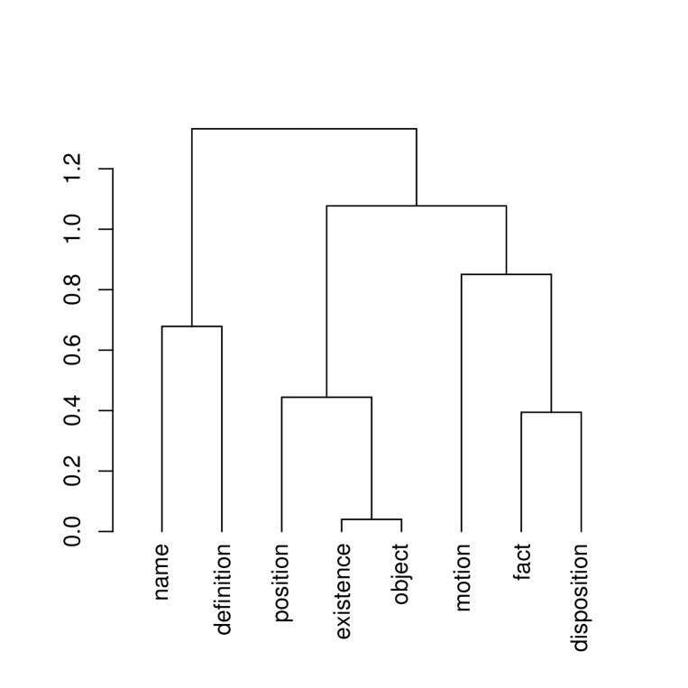
Figure 7: Hierarchical clustering of 8 terms. Data on which this was based: frequencies of occurrence of the 8 nouns in 24 successive, non-overlapping segments of Aristotle’s Categories.

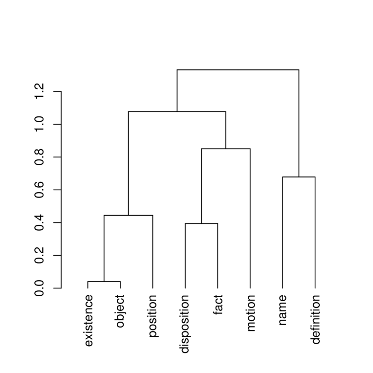
Figure 8: Dendrogram on 8 terms, isomorphic to the previous figure, Figure 7, but now with successively later agglomerations always represented by right child node. Apart from the labels of the initial pairwise agglomerations, this is otherwise a unique representation of the dendrogram (hence: “existence” and “object” can be interchanged; so can “disposition” and “fact”; and finally “name” and “disposition”). In the discussion we refer to this representation, with later agglomerations always parked to the right, as our canonical representation of the dendrogram.

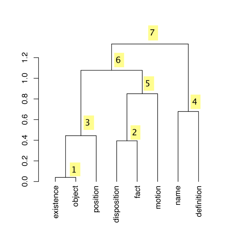
Figure 9: Dendrogram on 8 terms, as previous figure, Figure 8, with non-terminal nodes numbered in sequence. These will form the nodes of the oriented binary tree. We may consider one further node for completeness, 8 or $\infty$, located at an arbitrary location in the upper right.

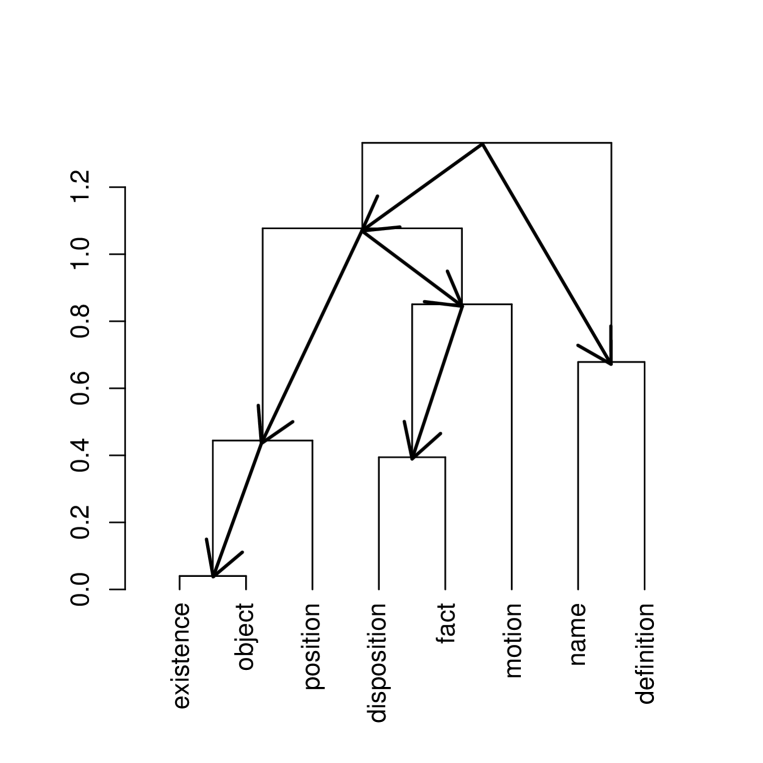
Figure 10: Oriented binary tree is superimposed on the dendrogram. The node at the arbitrary upper right location is not shown. The oriented binary tree defines an inorder or depth-first tree traversal.

5.2 Permutation Representation of a Hierarchy

There is an isomorphism between the class of hierarchic structures, termed unlabeled, ranked, binary, rooted trees, and the class of permutations used in symbolic dynamics. Each non-terminal node in the tree shown in Figure 7 has two child nodes. This is a dendrogram, representing a set of $n-1$ agglomerations based on $n$ initial data vectors.

Figure 7 shows a hierarchical clustering. Figure 8 shows a unique representation of the tree, termed a dendrogram, subject only to terminals being permutable in position relative to the first non-terminal cluster node.

A packed representation [73] or permutation representation of a dendrogram is derived as follows. Put a lower ranked subtree always to the left; and read off the oriented binary tree on non-terminal nodes. Then for any terminal node indexed by $i$, with the exception of the rightmost which will always be $n$, define $p(i)$ as the rank at which the terminal node is first united with some terminal node to its right.

For the dendrogram shown in Figure 10 (or Figures 8 or 9), the packed representation is: $(13625748)$. This is also an inorder traversal of the oriented binary tree (seen in Figure 10). The packed representation is a uniquely defined permutation of $1\dots n$.

Dendrograms (on $n$ terminals) of the sort shown in Figures 7–10 are labeled (see terminal node labels, “existence”, “object”, etc.) and ranked (ranks indicated in Figure 9). Consider when tree structure alone is of interest and we ignore the labels. Such dendrograms, called non-labeled, ranked (NL-R) in [56], are particularly interesting. They are isomorphic to either down-up permutations, or up-down permutations (both on $n-1$ elements). For the combinatorial properties of these permutations, and NL-R dendrograms, see the combinatorial sequence encyclopedia entry, A000111, at [75].

We see therefore how we are dealing with the group of up-down or down-up permutations.

6 Remarkable Symmetries in Very High Dimensional Spaces

In the work of [67, 68] it was shown how as ambient dimensionality increased distances became more and more ultrametric. That is to say, a hierarchical embedding becomes more and more immediate and direct as dimensionality increases. A better way of quantifying this phenomenon was developed in [59]. What this means is that there is inherent hierarchical structure in high dimensional data spaces.

It was shown experimentally in [67, 68, 59] how points in high dimensional spaces become increasingly equidistant with increase in dimensionality. Both [27] and [16] study Gaussian clouds in very high dimensions. The latter finds that “not only are the points [of a Gaussian cloud in very high dimensional space] on the convex hull, but all reasonable-sized subsets span faces of the convex hull. This is wildly different than the behavior that would be expected by traditional low-dimensional thinking”.

That very simple structures come about in very high dimensions is not as trivial as it might appear at first sight. Firstly, even very simple structures (hence with many symmetries) can be used to support fast and perhaps even constant time worst case proximity search [59]. Secondly, as shown in the machine learning framework by [27], there are important implications ensuing from the simple high dimensional structures. Thirdly, [62] shows that very high dimensional clustered data contain symmetries that in fact can be exploited to “read off” the clusters in a computationally efficient way. Fourthly, following [14], what we might want to look for in contexts of considerable symmetry are the “impurities” or small irregularities that detract from the overall dominant picture.

7 Conclusions

“My thesis has been that one path to the construction of a nontrivial theory of complex systems is by way of a theory of hierarchy.” ([74], p. 216.) Or again: “Human thinking (as well as many other information processes) is fundamentally a hierarchical process. … In our information modeling the main distinguishing feature of p-adic numbers is the treelike hierarchical structure. … [the work] is devoted to classical and quantum models of flows of hierarchically ordered information.” ([39], pp. xiii, xv.)

We have noted symmetry in many guises in the representations used, in the transformations applied, and in the transformed outputs. These symmetries are non-trivial too, in a way that would not be the case were we simply to look at classes of a partition and claim that cluster members were mutually similar in some way. We have seen how the p-adic or ultrametric framework provides significant focus and commonality of viewpoint.

In seeking (in a general way) and in determining (in a focused way) structure and regularity in data, we see that, in line with the insights and achievements of Klein, Weyl and Wigner, in data mining and data analysis we seek and determine symmetries in the data that express observed and measured reality. A very fundamental principle in much of statistics, signal processing and data analysis is that of sparsity but, as [4] show, by “codifying the inter-dependency structure” in the data new perspectives are opened up above and beyond sparsity.

References

- [1] C. Bandt. Ordinal time series analysis. Ecological Modelling, 182:229–238, 2005.
- [2] C. Bandt and B. Pompe. Permutation entropy: a natural complexity measure for time series. Physical Review Letters, 88:174102(4), 2002.
- [3] C. Bandt and F. Shiha. Order patterns in time series. Technical report, 2005. Preprint 3/2005, Institute of Mathematics, Greifswald, www.math-inf.uni-greifswald.de/bandt/pub.html.
- [4] R.G. Baraniuk, V. Cevher, M.F. Duarte, and C. Hegde. Model-based compressive sensing. 2008. http://arxiv.org/abs/0808.3572.
- [5] J.J. Benedetto and R.L. Benedetto. A wavelet theory for local fields and related groups. The Journal of Geometric Analysis, 14:423–456, 2004.
- [6] R.L. Benedetto. Examples of wavelets for local fields. In D. Larson C. Heil, P. Jorgensen, editor, Wavelets, Frames, and Operator Theory, Contemporary Mathematics Vol. 345, pages 27–47. 2004.
- [7] J.-P. Benzécri. La Taxinomie. Dunod, Paris, 2nd edition, 1979.
- [8] P.E. Bradley. Mumford dendrograms. Computer Journal, 2008. forthcoming, Advance Access online doi:10.1093/comjnl/bxm088.
- [9] L. Brekke and P.G.O. Freund. p-Adic numbers in physics. Physics Reports, 233:1–66, 1993.
- [10] P. Chakraborty. Looking through newly to the amazing irrationals. Technical report, 2005. arXiv: math.HO/0502049v1.
- [11] M. Costa, A.L. Goldberger, and C.-K. Peng. Multiscale entropy analysis of biological signals. Physical Review E, 71:021906(18), 2005.
- [12] F. Critchley and W. Heiser. Hierarchical trees can be perfectly scaled in one dimension. Journal of Classification, 5:5–20, 1988.
- [13] B.A. Davey and H.A. Priestley. Introduction to Lattices and Order. Cambridge University Press, 2nd edition, 2002.
- [14] F. Delon. Espaces ultramétriques. Journal of Symbolic Logic, 49:405–502, 1984.
- [15] S.B. Deutsch and J.J. Martin. An ordering algorithm for analysis of data arrays. Operations Research, 19:1350–1362, 1971.
- [16] D.L. Donoho and J. Tanner. Neighborliness of randomly-projected simplices in high dimensions. Proceedings of the National Academy of Sciences, 102:9452–9457, 2005.
- [17] B. Dragovich and A. Dragovich. p-Adic modelling of the genome and the genetic code. Computer Journal, 2007. forthcoming, Advance Access doi:10.1093/comjnl/bxm083.
- [18] R.A. Fisher. The use of multiple measurements in taxonomic problems. The Annals of Eugenics, pages 179–188, 1936.
- [19] R. Foote. An algebraic approach to multiresolution analysis. Transactions of the American Mathematical Society, 357:5031–5050, 2005.
- [20] R. Foote. Mathematics and complex systems. Science, 318:410–412, 2007.
- [21] R. Foote, G. Mirchandani, D. Rockmore, D. Healy, and T. Olson. A wreath product group approach to signal and image processing: Part I – multiresolution analysis. IEEE Transactions on Signal Processing, 48:102–132, 2000.
- [22] R. Foote, G. Mirchandani, D. Rockmore, D. Healy, and T. Olson. A wreath product group approach to signal and image processing: Part II – convolution, correlations and applications. IEEE Transactions on Signal Processing, 48:749–767, 2000.
- [23] P.G.O. Freund. p-Adic strings and their applications. In Z. Rakic B. Dragovich, A. Khrennikov and I. Volovich, editors, Proc. 2nd International Conference on p-Adic Mathematical Physics, pages 65–73. American Institute of Physics, 2006.
- [24] L. Gajić. On ultrametric space. Novi Sad Journal of Mathematics, 31:69–71, 2001.
- [25] B. Ganter and R. Wille. Formal Concept Analysis: Mathematical Foundations. Springer, 1999. Formale Begriffsanalyse. Mathematische Grundlagen, Springer, 1996.
- [26] F.Q. Gouvêa. p-Adic Numbers: An Introduction. Springer, 2003.
- [27] P. Hall, J.S. Marron, and A. Neeman. Geometric representation of high dimensional, low sample size data. Journal of the Royal Statistical Society B, 67:427–444, 2005.
- [28] P. Hitzler and A.K. Seda. The fixed-point theorems of Priess-Crampe and Ribenboim in logic programming. Fields Institute Communications, 32:219–235, 2002.
- [29] A.K. Jain and R.C. Dubes. Algorithms For Clustering Data. Prentice-Hall, 1988.
- [30] A.K. Jain, M.N. Murty, and P.J. Flynn. Data clustering: a review. ACM Computing Surveys, 31:264–323, 1999.
- [31] M.F. Janowitz. An order theoretic model for cluster analysis. SIAM Journal on Applied Mathematics, 34:55–72, 1978.
- [32] M.F. Janowitz. Cluster analysis based on abstract posets. Technical report, 2005–2006. http://dimax.rutgers.edu/melj.
- [33] M. Jansen, G.P. Nason, and B.W. Silverman. Multiscale methods for data on graphs and irregular multidimensional situations. Journal of the Royal Statistical Society B, 71:97–126, 2009.
- [34] S.C. Johnson. Hierarchical clustering schemes. Psychometrika, 32:241–254, 1967.
- [35] K. Keller and H. Lauffer. Symbolic analysis of high-dimensional time series. International Journal of Bifurcation and Chaos, 13:2657–2668, 2003.
- [36] K. Keller, H. Lauffer, and M. Sinn. Ordinal analysis of EEG time series. Chaos and Complexity Letters, 2:247–258, 2007.
- [37] K. Keller and M. Sinn. Ordinal analysis of time series. Physica A, 356:114–120, 2005.
- [38] K. Keller and M. Sinn. Ordinal symbolic dynamics. 2005. Technical Report A-05-14, www.math.mu-luebeck.de/publikationen/pub2005.shtml.
- [39] A.Yu. Khrennikov. Information Dynamics in Cognitive, Psychological, Social and Anomalous Phenomena. Kluwer, 2004.
- [40] A.Yu. Khrennikov. Gene expression from polynomial dynamics in the 2-adic information space. Technical report, 2006. arXiv:q-bio/06110682v2.
- [41] F. Klein. A comparative review of recent researches in geometry. Bull. New York Math. Soc., 2:215–249, 1892–1893. Vergleichende Betrachtungen über neuere geometrische Forschungen, 1872, translated by M.W. Haskell.
- [42] S. V. Kozyrev. Wavelet theory as p-adic spectral analysis. Izvestiya: Mathematics, 66:367–376, 2002.
- [43] S. V. Kozyrev. Wavelets and spectral analysis of ultrametric pseudodifferential operators. Sbornik: Mathematics, 198:97–116, 2007.
- [44] M. Krasner. Nombres semi-réels et espaces ultramétriques. Comptes-Rendus de l’Académie des Sciences, Tome II, 219:433, 1944.
- [45] V. Latora and M. Baranger. Kolmogorov-Sinai entropy rate versus physical entropy. Physical Review Letters, 82:520, 1999.
- [46] I.C. Lerman. Classification et Analyse Ordinale des Données. Dunod, Paris, 1981.
- [47] A. Levy. Basic Set Theory. Dover, Mineola, NY, 2002. (Springer, 1979).
- [48] S.C. Madeira and A.L. Oliveira. Biclustering algorithms for biological data analysis: a survey. IEEE/ACM Transactions on Computational Biology and Bioinformatics, 1:24–45, 2004.
- [49] S.T. March. Techniques for structuring database records. Computing Surveys, 15:45–79, 1983.
- [50] W.T. McCormick, P.J. Schweitzer, and T.J. White. Problem decomposition and data reorganization by a clustering technique. Operations Research, 20:993–1009, 1982.
- [51] I. Van Mechelen, H.-H. Bock, and P. De Boeck. Two-mode clustering methods: a structured overview. Statistical Methods in Medical Research, 13:363–394, 2004.
- [52] B. Mirkin. Mathematical Classification and Clustering. Kluwer, 1996.
- [53] B. Mirkin. Clustering for Data Mining. Chapman and Hall/CRC, Boca Raton, FL, 2005.
- [54] F. Murtagh. A survey of recent advances in hierarchical clustering algorithms. Computer Journal, 26:354–359, 1983.
- [55] F. Murtagh. Complexities of hierarchic clustering algorithms: state of the art. Computational Statistics Quarterly, 1:101–113, 1984.
- [56] F. Murtagh. Counting dendrograms: a survey. Discrete Applied Mathematics, 7:191–199, 1984.
- [57] F. Murtagh. Multidimensional Clustering Algorithms. Physica-Verlag, Heidelberg and Vienna, 1985.
- [58] F. Murtagh. Comments on: Parallel algorithms for hierarchical clustering and cluster validity. IEEE Transactions on Pattern Analysis and Machine Intelligence, 14:1056–1057, 1992.
- [59] F. Murtagh. On ultrametricity, data coding, and computation. Journal of Classification, 21:167–184, 2004.
- [60] F. Murtagh. Identifying the ultrametricity of time series. European Physical Journal B, 43:573–579, 2005.
- [61] F. Murtagh. The Haar wavelet transform of a dendrogram. Journal of Classification, 24:3–32, 2007.
- [62] F. Murtagh. The remarkable simplicity of very high dimensional data: application to model-based clustering. Journal of Classification, 2007. Submitted.
- [63] F. Murtagh. The correspondence analysis platform for uncovering deep structure in data and information (sixth Annual Boole Lecture). Computer Journal, 2008. forthcoming, Advance Access doi:10.1093/comjnl/bxn045.
- [64] F. Murtagh, G. Downs, and P. Contreras. Hierarchical clustering of massive, high dimensional data sets by exploiting ultrametric embedding. SIAM Journal on Scientific Computing, 30:707–730, 2008.
- [65] F. Murtagh, J.-L. Starck, and M. Berry. Overcoming the curse of dimensionality in clustering by means of the wavelet transform. Computer Journal, 43:107–120, 2000.
- [66] A. Ostrowski. Über einige Lösungen der Funktionalgleichung . Acta Mathematica, 41:271–284, 1918.
- [67] R. Rammal, J.C. Angles d’Auriac, and B. Doucot. On the degree of ultrametricity. Le Journal de Physique – Lettres, 46:L–945–L–952, 1985.
- [68] R. Rammal, G. Toulouse, and M.A. Virasoro. Ultrametricity for physicists. Reviews of Modern Physics, 58:765–788, 1986.
- [69] H. Reiter and J.D. Stegeman. Classical Harmonic Analysis and Locally Compact Groups. Oxford University Press, Oxford, 2nd edition, 2000.
- [70] A.C.M. Van Rooij. Non-Archimedean Functional Analysis. Marcel Dekker, 1978.
- [71] W.H. Schikhof. Ultrametric Calculus. Cambridge University Press, Cambridge, 1984. (Chapters 18, 19, 20, 21).
- [72] A.K. Seda and P. Hitzler. Generalized distance functions in the theory of computation. Computer Journal, 2008. forthcoming, Advance Access doi:10.1093/comjnl/bxm108.
- [73] R. Sibson. Slink: an optimally efficient algorithm for the single-link cluster method. Computer Journal, 16:30–34, 1980.
- [74] H.A. Simon. The Sciences of the Artificial. MIT Press, Cambridge, MA, 1996.
- [75] N.J.A. Sloane. OEIS – On-Line Encyclopedia of Integer Sequences. Technical report, 2006. http://www.research.att.com/njas/sequences/Seis.html, Sequence A000111: http://www.research.att.com/njas/sequences/A000111.
- [76] D. Steinley. K-means clustering: a half-century synthesis. British Journal of Mathematical and Statistical Psychology, 59:1–3, 2006.
- [77] D. Steinley and M.J. Brusco. Initializing K-means batch clustering: a critical evaluation of several techniques. Journal of Classification, 24:99–121, 2007.
- [78] Wu-Ki Tung. Group Theory in Physics. World Scientific, 1985.
- [79] S.S. Vempala. The Random Projection Method. American Mathematical Society, 2004. Vol. 65, DIMACS Series in Discrete Mathematics and Theoretical Computer Science.
- [80] I.V. Volovich. Number theory as the ultimate physical theory. Technical report, 1987. Preprint No. TH 4781/87, CERN, Geneva.
- [81] I.V. Volovich. p-Adic string. Classical Quantum Gravity, 4:L83–L87, 1987.
- [82] W. Weckesser. Symbolic dynamics in mathematics, physics, and engineering, based on a talk by N. Tuffilaro. Technical report, 1997. http://www.ima.umn.edu/weck/nbt/nbt.ps.
- [83] H. Weyl. Symmetry. Princeton University Press, 1983.
- [84] Rui Xu and D. Wunsch. Survey of clustering algorithms. IEEE Transactions on Neural Networks, 16:645–678, 2005.