A theorem concerning twisted and untwisted partition functions in $U(N)$ and $SU(N)$ lattice gauge theories

Abstract

In order to get a clue to understanding the volume-dependence of vortex free energy (which is defined as the ratio of the twisted against the untwisted partition function), we investigate the relation between vortex free energies defined on lattices of different sizes. An equality is derived through a simple calculation which equates a general linear combination of vortex free energies defined on a lattice to that on a smaller lattice. The couplings in the denominator and in the numerator however shows a discrepancy, and we argue that it vanishes in the thermodynamic limit. Comparison between our result and the work of Tomboulis is also presented. In the appendix we carefully examine the proof of quark confinement by Tomboulis and summarize its loopholes.
   PACS numbers: 11.15.Ha, 12.38.Aw
   key words: lattice gauge theory, vortex free energy, Migdal-Kadanoff transformation, quark confinement

§1 Introduction

Quark confinement, or (more generally) color confinement is one of the most long-standing problems in theoretical physics [1]. So far many proposals have been made concerning the nonperturbative dynamics of QCD which yield confinement, including the dual superconductivity scenario [2] and center vortex scenario [3] (see [4] for a review), but a truly satisfying picture seems to be still missing and precise relationship between different scenarios is elusive. In the lattice gauge theory it is formulated as the area law of the Wilson loop in the absence of dynamical fermions, which indicates a linear static potential $V(r)\propto r$ between infinitely heavy quark and anti-quark. So far the area law has been rigorously proved (in the physicists’ sense) for quite restricted models [5, 6, 7] although it has been numerically checked by Monte Carlo simulations for years [8].

The concept of center vortices in non-abelian gauge theories was introduced long time ago [3, 6, 7, 9]. This picture successfully explains many aspects of infra-red properties of Yang-Mills theory at the qualitative level, and also at the quantitative level it is reported that Monte Carlo simulations show that the value of the string tension can be mostly recovered by the effective vortex degrees of freedom (‘P-vortex’) which one extracts via a procedure called ‘center projection’ [10]. It is also reported that quenching P-vortices leads to the disappearance of area law and the restoration of chiral symmetry at the same time [11], which suggests that the vortices represent infra-red properties of the theory in a comprehensive manner.

In addition, the picture that the percolation of center vortices leads to the area law has a firm ground based on the Tomboulis-Yaffe inequality [12]:

$$\langle W(C)\rangle\leq 2\Big{\{}\displaystyle\frac{\,1\,^{\mathstrut}}{\,2\,_{\mathstrut}}(1-{\mathrm{e}}^{-F_{v}})\Big{\}}^{A_{C}/L_{\mu}L_{\nu}}$$ (1)

for $SU(2)$, which can be proved rigorously on the lattice. Here $A_{C}$ denotes the area enclosed by a rectangle $C$ which lies in a $[\mu,\nu]$-plane, $W(C)$ is the Wilson loop associated to $C$ in the fundamental representation and $L_{\mu}$ is the length of the lattice in the $\mu$-th direction. According to this inequality the area law of the l.h.s. follows if the vortex free energy $F_{v}$ vanishes in the thermodynamic limit in such a way that $F_{v}\approx{\mathrm{e}}^{-\rho L_{\mu}L_{\nu}}$. The quantity $\rho$ gives a lower bound of the string tension, and is called the ’t Hooft string tension. This behavior of $F_{v}$ is verified within the strong coupling cluster expansion [13] and is also supported by Monte Carlo simulations [14]. So it is worthwhile to study the volume dependence of $F_{v}$ particularly at intermediate and weak couplings.

In this work we attempt to make a connection between vortex free energies defined on lattices of different sizes. The set up of this note is as follows. In §2 we establish an equality which relates the ratio of the ordinary and the twisted partition function on a lattice to that on a smaller lattice, without any restriction on the coupling strength. The cost is that there is a slight discrepancy between the couplings in the denominator and in the numerator, but it can be shown to tend to zero in the thermodynamic limit. In §3 we examine the relation between our result and the work of Tomboulis [15]. Final section is devoted to summary and concluding remarks. In the appendix we carefully examine the proof of quark confinement in ref.[15], listing its loopholes.

In view of the serious scarcity of rigorous results in this area of research, our analytical work which involves no approximation seems to be of basic importance, and we hope that this result will serve as a building block of the proof of quark confinement in the future.

§2 The main result

Let us begin by describing the basic set-up of lattice gauge theory. Let $\Lambda$ a $d$-dimensional hypercubic lattice of length $L_{\mu}\,(\mu=1,\dots,d)$ in each direction with the periodic boundary condition imposed. Let $\Lambda^{(n)}$ a $d$-dimensional hypercubic lattice of length $L_{\mu}/b^{n}\,(\mu=1\dots,d)$ in each direction with a parameter $b\in\mathbf{N}$. The number of plaquettes in $\Lambda$ is denoted by $|\Lambda|$. The partition function on the lattice $\Lambda$ is defined as

$$Z_{\Lambda}(\{c_{r}\})\equiv\displaystyle\int\prod_{b\in\Lambda}dU_{b}\prod_{p\subset\Lambda}f_{p}(U_{p})\equiv\displaystyle\int\prod_{b\in\Lambda}dU_{b}\prod_{p\subset\Lambda}\Big{[}1+\displaystyle\sum_{r\not=\mathbf{1}}d_{r}c_{r}(\beta)\chi_{r}(U_{p})\Big{]},$$ (2)

where $dU$ is the normalized Haar measure of gauge group $G$ and $U_{p}$ is a plaquette variable; $U_{p}\equiv U_{x,\mu}U_{x+\mu,\nu}U_{x+\nu,\mu}^{\dagger}U^{\dagger}_{x,\nu}$. In what follows we only consider $G=U(N)$ and $SU(N)$. The subscript $r$ labels irreducible representations of $G$ and $d_{r}$ is the dimension, $\chi_{r}$ is the character of the $r$-th representation ($\mathbf{1}$ is the trivial representation). The coefficients $\{c_{r}(\beta)\}$ can be determined through the character expansion of (for instance) the Wilson action:

$${\mathrm{e}}^{\beta{\mathrm{Re\,Tr\,}}U}\Big{/}\displaystyle\int dU^{\prime}\,{\mathrm{e}}^{\beta{\mathrm{Re\,Tr\,}}U^{\prime}}\equiv f_{p}(U)=1+\displaystyle\sum_{r\not=\mathbf{1}}d_{r}c_{r}(\beta)\chi_{r}(U).$$ (3)

It can be checked that $c_{r}\geq 0$ holds for every $r$, which guarantees the reflection positivity of the measure and unitarity of the corresponding quantum-mechanical system.

Multiplying a plaquette variable $U_{p}$ by a nontrivial element of the center of the gauge group is called a twist which, in physical terms, generates a magnetic flux piercing the plaquette. Let $C(G)$ denote the center of $G$; $C(SU(N))=Z_{N}$ and $C(U(N))=U(1)$. The twisted partition function reads

$$Z^{g}_{\Lambda}(\{c_{r}\}) \equiv\displaystyle\int\prod_{b\in\Lambda}dU_{b}\prod_{p\subset\mathcal{V}}f_{p}(gU_{p})\prod_{p^{\prime}\subset\Lambda\setminus\mathcal{V}}f_{p}(U_{p^{\prime}}),\hskip 20.0ptg\in C(G).$$ (4)

Here $\mathcal{V}$ is a set of stacked plaquettes which winds around $(d-2)$ of the $d$ periodic directions of $\Lambda$ forming a $(d-2)$-dimensional torus on the dual lattice. (Using reflection positivity one can show $Z^{g}_{\Lambda}\leq Z_{\Lambda}$ [17] and the vortex free energy $F_{v}^{g}$ associated to the twist by $g$ is defined by ${\mathrm{e}}^{-F_{v}^{g}}=Z^{g}_{\Lambda}/Z_{\Lambda}$.) Our main result is as follows:

Theorem 1.

Let $H$ an arbitrary discrete subgroup of U(1) for $G=U(N)$ and $H=Z_{N}$ for $G=SU(N)$. Fix a set of positive coefficients $\{c_{r}^{\prime}\}$ and $n\in\mathbf{N}$, and choose a constant $A^{g}>0$ for each $g\in H$ arbitrarily. Then there exists $\lambda(\{c_{r}^{\prime}\})>0$ such that for any $0<\alpha<\lambda(\{c_{r}^{\prime}\})$ and for sufficiently large $|\Lambda|$ there exists $\overline{\alpha}_{\Lambda}\equiv\overline{\alpha}_{\Lambda}(\alpha,\{c_{r}\},\{c^{\prime}_{r}\})$ such that $\left|\alpha-\overline{\alpha}_{\Lambda}\right|\leq O\Big{(}\displaystyle\frac{\,1\,^{\mathstrut}}{\,|\Lambda|\,_{\mathstrut}}\Big{)}$ and

$$\frac{\,\mathcal{Z}_{\Lambda}(\{c_{r}\})\,^{\mathstrut}}{\,Z_{\Lambda}(\{c_{r}\})\,_{\mathstrut}}=\displaystyle\frac{\,\mathcal{Z}_{\Lambda^{(n)}}(\{\alpha c^{\prime}_{r}\})\,^{\mathstrut}}{\,Z_{\Lambda^{(n)}}(\{\overline{\alpha}_{\Lambda}c^{\prime}_{r}\})\,_{\mathstrut}}$$ (5)

with

$$\mathcal{Z}_{\Lambda}(\{c_{r}\})\equiv\displaystyle\sum_{g\in H}A^{g}Z^{g}_{\Lambda}(\{c_{r}\}).$$ (6)

Proof.

Let us define functions $C_{\Lambda}(\alpha,\{c_{r}\},\{c^{\prime}_{r}\}),\,\mathcal{C}_{\Lambda}(\alpha,\{c_{r}\},\{c^{\prime}_{r}\})$ by

$$Z_{\Lambda}(\{c_{r}\}) ={\mathrm{e}}^{C_{\Lambda}(\alpha,\{c_{r}\},\{c^{\prime}_{r}\})|\Lambda|}Z_{\Lambda^{(n)}}(\{\alpha c^{\prime}_{r}\}),$$ (7)

$$\mathcal{Z}_{\Lambda}(\{c_{r}\}) ={\mathrm{e}}^{\mathcal{C}_{\Lambda}(\alpha,\{c_{r}\},\{c^{\prime}_{r}\})|\Lambda|}\mathcal{Z}_{\Lambda^{(n)}}(\{\alpha c^{\prime}_{r}\}).$$ (8)

Taking the ratio of (7) and (8) yields

$$\frac{\,\mathcal{Z}_{\Lambda}(\{c_{r}\})\,^{\mathstrut}}{\,Z_{\Lambda}(\{c_{r}\})\,_{\mathstrut}}={\mathrm{e}}^{\{\mathcal{C}_{\Lambda}(\alpha,\{c_{r}\},\{c^{\prime}_{r}\})-C_{\Lambda}(\alpha,\{c_{r}\},\{c^{\prime}_{r}\})\}|\Lambda|}\displaystyle\frac{\,\mathcal{Z}_{\Lambda^{(n)}}(\{\alpha c^{\prime}_{r}\})\,^{\mathstrut}}{\,Z_{\Lambda^{(n)}}(\{\alpha c^{\prime}_{r}\})\,_{\mathstrut}}.$$ (9)

From (9) and $A^{e}<\displaystyle\frac{\,\mathcal{Z}_{\Lambda}(\{c_{r}\})\,^{\mathstrut}}{\,Z_{\Lambda}(\{c_{r}\})\,_{\mathstrut}},\,\displaystyle\frac{\,\mathcal{Z}_{\Lambda^{(n)}}(\{\alpha c^{\prime}_{r}\})\,^{\mathstrut}}{\,Z_{\Lambda^{(n)}}(\{\alpha c^{\prime}_{r}\})\,_{\mathstrut}}<\displaystyle\sum_{g\in H}A^{g}$ we have

$$\left|\mathcal{C}_{\Lambda}(\alpha,\{c_{r}\},\{c^{\prime}_{r}\})-C_{\Lambda}(\alpha,\{c_{r}\},\{c^{\prime}_{r}\})\right|\leq O\Big{(}\displaystyle\frac{\,1\,^{\mathstrut}}{\,|\Lambda|\,_{\mathstrut}}\Big{)}.$$ (10)

Now let us rewrite (7) into more useful form:

$$\frac{\,1\,^{\mathstrut}}{\,|\Lambda|\,_{\mathstrut}}\log Z_{\Lambda}(\{c_{r}\})=C_{\Lambda}(\alpha,\{c_{r}\},\{c^{\prime}_{r}\})+\displaystyle\frac{\,|\Lambda^{(n)}|\,^{\mathstrut}}{\,|\Lambda|\,_{\mathstrut}}\Bigg{[}\displaystyle\frac{\,1\,^{\mathstrut}}{\,|\Lambda^{(n)}|\,_{\mathstrut}}\log Z_{\Lambda^{(n)}}(\{\alpha c^{\prime}_{r}\})\Bigg{]}.$$ (11)

The l.h.s. has a well-defined thermodynamic limit which we denote by $z(\{c_{r}\})$. It is well known [13, 18] that strong coupling cluster expansion has a non-vanishing radius of convergence which is independent of the total volume, so there exists $\lambda(\{c_{r}^{\prime}\})$ such that $[\dots]$ in the r.h.s. of (11) can be well approximated by the lowest order strong coupling cluster expansion for $0<\alpha<\lambda(\{c_{r}^{\prime}\})$, giving

$$z(\{c_{r}\})=C_{\infty}(\alpha,\{c_{r}\},\{c^{\prime}_{r}\})+\displaystyle\frac{\,a_{d}\,^{\mathstrut}}{\,b^{nd}\,_{\mathstrut}}\displaystyle\sum_{r\not=\mathbf{1}}d_{r}^{2}\big{(}\alpha c_{r}^{\prime}\big{)}^{6}+O\big{(}\big{(}\alpha c_{r}^{\prime}\big{)}^{10}\big{)},$$ (12)

where $a_{3}\equiv\displaystyle\frac{\,1\,^{\mathstrut}}{\,3\,_{\mathstrut}},\,a_{4}\equiv\displaystyle\frac{\,2\,^{\mathstrut}}{\,3\,_{\mathstrut}}$ and we denominated $C_{\infty}(\alpha,\{c_{r}\},\{c^{\prime}_{r}\})\equiv\displaystyle\lim_{|\Lambda|\to\infty}C_{\Lambda}(\alpha,\{c_{r}\},\{c^{\prime}_{r}\})$. Thus

$$\hskip 20.0pt\displaystyle\frac{\,dC_{\infty}(\alpha,\{c_{r}\},\{c^{\prime}_{r}\})\,^{\mathstrut}}{\,d\alpha\,_{\mathstrut}}\simeq-C_{0}\alpha^{5}\hskip 30.0pt{\rm{for}}\ \ \ 0<\alpha<\lambda(\{c_{r}^{\prime}\}),$$ (13)

where the factor $C_{0}$ is independent of the volume. Therefore $\Big{|}\displaystyle\frac{\,dC_{\Lambda}\,^{\mathstrut}}{\,d\alpha\,_{\mathstrut}}\Big{|}$ has a non-vanishing lower bound for arbitrarily large $|\Lambda|$. From this fact and (10) follows that if $|\Lambda|$ is sufficiently large there exists $\overline{\alpha}_{\Lambda}(\alpha,\{c_{r}\},\{c^{\prime}_{r}\})$ such that $\left|\alpha-\overline{\alpha}_{\Lambda}\right|\leq O\Big{(}\displaystyle\frac{\,1\,^{\mathstrut}}{\,|\Lambda|\,_{\mathstrut}}\Big{)}$ and $\mathcal{C}_{\Lambda}(\alpha,\{c_{r}\},\{c^{\prime}_{r}\})=C_{\Lambda}(\overline{\alpha}_{\Lambda},\{c_{r}\},\{c^{\prime}_{r}\})$. Hence (5) is proved. ∎

One can relax the condition $\{A^{g}>0\,|\,g\in H\}$ within a scope which does not affect the existence of a strictly positive lower bound for $\displaystyle\frac{\,\mathcal{Z}_{\Lambda}(\{c_{r}\})\,^{\mathstrut}}{\,Z_{\Lambda}(\{c_{r}\})\,_{\mathstrut}}$.

Note that $\alpha$ and $\{c_{r}^{\prime}\}$ have no dependence on $\{c_{r}\}$, for they are parameters we introduced by hand. As the free energy density $z(\{c_{r}\})$ in the l.h.s. of (12) is a quantity which reflects the phase structure of the model, it is not necessarily analytic in $\{c_{r}\}$ and in $\beta$. In the r.h.s. of (12), such a nonanalyticity in $\{c_{r}\}$ resides in $C_{\infty}(\alpha,\{c_{r}\},\{c^{\prime}_{r}\})$ simply because the rest of the r.h.s. of (12) is independent of $\{c_{r}\}$. Note also that $C_{\infty}(\alpha,\{c_{r}\},\{c^{\prime}_{r}\})$ is Taylor-expandable and analytic in $\alpha$; the analyticity in $\alpha$ and a possible nonanalyticity in $\{c_{r}\}$ should be strictly distinguished.

Let us look at (5) in more detail. Since $\overline{\alpha}_{\Lambda}$ converges to $\alpha$ in the thermodynamic limit, one may be tempted to argue that $\displaystyle\lim_{|\Lambda|\to\infty}\displaystyle\frac{\,\mathcal{Z}_{\Lambda}(\{c_{r}\})\,^{\mathstrut}}{\,Z_{\Lambda}(\{c_{r}\})\,_{\mathstrut}}$ is independent of $\{c_{r}\}$ because

$$\lim_{|\Lambda|\to\infty}\displaystyle\frac{\,\mathcal{Z}_{\Lambda}(\{c_{r}\})\,^{\mathstrut}}{\,Z_{\Lambda}(\{c_{r}\})\,_{\mathstrut}}=\displaystyle\lim_{|\Lambda|\to\infty}\displaystyle\frac{\,\mathcal{Z}_{\Lambda^{(n)}}(\{\alpha c^{\prime}_{r}\})\,^{\mathstrut}}{\,Z_{\Lambda^{(n)}}(\{\overline{\alpha}_{\Lambda}c^{\prime}_{r}\})\,_{\mathstrut}}=\displaystyle\lim_{|\Lambda|\to\infty}\displaystyle\frac{\,\mathcal{Z}_{\Lambda^{(n)}}(\{\alpha c^{\prime}_{r}\})\,^{\mathstrut}}{\,Z_{\Lambda^{(n)}}(\{\alpha c^{\prime}_{r}\})\,_{\mathstrut}}.$$ (14)

It would be valuable to clarify why this claim is incorrect. Let us rewrite (5) as

$$\frac{\,\mathcal{Z}_{\Lambda}(\{c_{r}\})\,^{\mathstrut}}{\,Z_{\Lambda}(\{c_{r}\})\,_{\mathstrut}}=\displaystyle\frac{\,\mathcal{Z}_{\Lambda^{(n)}}(\{\alpha c^{\prime}_{r}\})\,^{\mathstrut}}{\,Z_{\Lambda^{(n)}}(\{\alpha c^{\prime}_{r}\})\,_{\mathstrut}}\displaystyle\frac{\,Z_{\Lambda^{(n)}}(\{\alpha c^{\prime}_{r}\})\,^{\mathstrut}}{\,Z_{\Lambda^{(n)}}(\{\overline{\alpha}_{\Lambda}c^{\prime}_{r}\})\,_{\mathstrut}}.$$ (15)

$\left|\alpha-\overline{\alpha}_{\Lambda}\right|\leq O\Big{(}\displaystyle\frac{\,1\,^{\mathstrut}}{\,|\Lambda|\,_{\mathstrut}}\Big{)}$ allows us to write $\overline{\alpha}_{\Lambda}=\alpha+\displaystyle\frac{\,\gamma_{\Lambda}(\alpha,\{c_{r}\},\{c^{\prime}_{r}\})\,^{\mathstrut}}{\,|\Lambda^{(n)}|\,_{\mathstrut}}$ with $|\gamma_{\Lambda}|\leq O(1)$. For $0<\alpha,\,\overline{\alpha}_{\Lambda}<\lambda(\{c^{\prime}_{r}\})$ we may apply the convergent cluster expansion to $\log Z_{\Lambda^{(n)}}(\{\alpha c^{\prime}_{r}\})$ and $\log Z_{\Lambda^{(n)}}(\{\overline{\alpha}_{\Lambda}c^{\prime}_{r}\})$ to obtain

$$\displaystyle\frac{\,Z_{\Lambda^{(n)}}(\{\alpha c^{\prime}_{r}\})\,^{\mathstrut}}{\,Z_{\Lambda^{(n)}}(\{\overline{\alpha}_{\Lambda}c^{\prime}_{r}\})\,_{\mathstrut}} \equiv\exp\left[|\Lambda^{(n)}|\left(\displaystyle\frac{\,1\,^{\mathstrut}}{\,|\Lambda^{(n)}|\,_{\mathstrut}}\log Z_{\Lambda^{(n)}}(\{\alpha c^{\prime}_{r}\})-\displaystyle\frac{\,1\,^{\mathstrut}}{\,|\Lambda^{(n)}|\,_{\mathstrut}}\log Z_{\Lambda^{(n)}}(\{\overline{\alpha}_{\Lambda}c^{\prime}_{r}\})\right)\right]$$ (16)

$$=\exp\left[|\Lambda^{(n)}|\displaystyle\sum_{r,k}s_{r,k}\left\{(\alpha c^{\prime}_{r})^{k}-(\overline{\alpha}_{\Lambda}c^{\prime}_{r})^{k}\right\}\right]$$ (17)

$$=\exp\left[-\gamma_{\Lambda}\displaystyle\sum_{r,k}s_{r,k}(c^{\prime}_{r})^{k}k\alpha^{k-1}+O\Big{(}\displaystyle\frac{\,1\,^{\mathstrut}}{\,|\Lambda^{(n)}|\,_{\mathstrut}}\Big{)}\right]$$ (18)

$$\longrightarrow\ \exp\left[-\gamma_{\infty}\displaystyle\sum_{r,k}s_{r,k}(c^{\prime}_{r})^{k}k\alpha^{k-1}\right]\hskip 40.0pt\textrm{as}\ |\Lambda|\to\infty.$$ (19)

$\{s_{r,k}\}$ are coefficients of clusters. (19) clearly shows how the discrepancy between $\alpha$ and $\overline{\alpha}_{\Lambda}$ persists in the thermodynamic limit and we now see why the previous claim is incorrect. Note, furthermore, that the function $\gamma_{\infty}(\alpha,\{c_{r}\},\{c^{\prime}_{r}\})\equiv\displaystyle\lim_{|\Lambda|\to\infty}\gamma_{\Lambda}(\alpha,\{c_{r}\},\{c^{\prime}_{r}\})$ is not necessarily analytic in $\{c_{r}\}$; information in the l.h.s. of (15) about the phase structure of the model is now packaged within a single unknown function $\gamma_{\infty}$.

We would like to comment on a possible path from theorem 1 to a proof of quark confinement. Suppose $G=SU(N)$.

Theorem 2.

If $N$-ality of the $r$-th representation is non-zero, we have

$$|\langle W_{r}(C)\rangle|\leq 2\Big{\{}1-\displaystyle\frac{\,1\,^{\mathstrut}}{\,N\,_{\mathstrut}}\displaystyle\sum_{g\in Z_{N}}\displaystyle\frac{\,Z_{\Lambda}^{g}(\{c_{r}\})\,^{\mathstrut}}{\,Z_{\Lambda}(\{c_{r}\})\,_{\mathstrut}}\Big{\}}^{A_{C}/L_{\mu}L_{\nu}}$$ (20)

for the normalized Wilson loop $W_{r}(C)\equiv\displaystyle\frac{\,1\,^{\mathstrut}}{\,d_{r}\,{}_{\mathstrut}}\chi_{r}\big{(}\mathcal{P}\prod_{b\in C}U_{b}\big{)}$, where $\mathcal{P}$ implies path-ordering and $\langle\dots\rangle$ in the l.h.s. is the expectation value w.r.t. $Z_{\Lambda}(\{c_{r}\})$.

Detailed proof of (20) is given in ref.[17] and we skip it here. Let $A^{g}=\displaystyle\frac{\,1\,^{\mathstrut}}{\,N\,_{\mathstrut}}$ for ${}^{\forall}g\in Z_{N}$ and assume that
$C_{\Lambda}(\alpha_{0},\{c_{r}\},\{c^{\prime}_{r}\})=\mathcal{C}_{\Lambda}(\alpha_{0},\{c_{r}\},\{c^{\prime}_{r}\})$ hold for some $\alpha_{0}\in[0,\lambda(\{c^{\prime}_{r}\})]$. Substituting $\alpha=\alpha_{0}$ into (9) gives

$$\frac{\,\mathcal{Z}_{\Lambda}(\{c_{r}\})\,^{\mathstrut}}{\,Z_{\Lambda}(\{c_{r}\})\,_{\mathstrut}}\Big{(}\equiv\displaystyle\frac{\,1\,^{\mathstrut}}{\,N\,_{\mathstrut}}\displaystyle\sum_{g\in Z_{N}}\displaystyle\frac{\,Z_{\Lambda}^{g}(\{c_{r}\})\,^{\mathstrut}}{\,Z_{\Lambda}(\{c_{r}\})\,_{\mathstrut}}\Big{)}=\displaystyle\frac{\,\mathcal{Z}_{\Lambda^{(n)}}(\{\alpha_{0}c^{\prime}_{r}\})\,^{\mathstrut}}{\,Z_{\Lambda^{(n)}}(\{\alpha_{0}c^{\prime}_{r}\})\,_{\mathstrut}}.$$ (21)

From the definition of $\lambda(\{c^{\prime}_{r}\})$, the r.h.s. can be estimated by the convergent cluster expansion, giving

$$\frac{\,\mathcal{Z}_{\Lambda^{(n)}}(\{\alpha_{0}c^{\prime}_{r}\})\,^{\mathstrut}}{\,Z_{\Lambda^{(n)}}(\{\alpha_{0}c^{\prime}_{r}\})\,_{\mathstrut}}\approx 1-O({\mathrm{e}}^{-\rho L_{\mu}^{(n)}L_{\nu}^{(n)}})=1-O({\mathrm{e}}^{-\rho L_{\mu}L_{\nu}/b^{2n}})$$ (22)

where $L_{\mu}^{(n)}\equiv L_{\mu}/b^{n}$ is the length of $\Lambda^{(n)}$ in $\mu$-th direction. Inserting (22) into (20) we obtain

$$|\langle W_{r}(C)\rangle|\lesssim{\mathrm{e}}^{-\rho A_{C}/b^{2n}},$$ (23)

hence the quark confinement follows. Whether the above strategy (to search for the intersection point of curves $\mathcal{C}_{\Lambda}(\cdot,\{c_{r}\},\{c^{\prime}_{r}\})$ and $C_{\Lambda}(\cdot,\{c_{r}\},\{c^{\prime}_{r}\})$) is viable or not remains to be seen.

§3 Comparison with Tomboulis’ approach

The purpose of this section is to elucidate the simplification and generalization achieved in the previous section, through the comparison with the approach in ref.[15], where only $G=SU(2)$ is treated explicitly. The whole argument in ref.[15] seems to rest on the Migdal-Kadanoff(MK) renormalization group transformation below:

$$c_{j}(n+1)\equiv\left(\displaystyle\frac{\,\displaystyle\int dU\big{[}f_{p}(U,n)\big{]}^{b^{d-2}}\displaystyle\frac{\,1\,^{\mathstrut}}{\,d_{j}\,{}_{\mathstrut}}\chi_{j}(U)\,^{\mathstrut}}{\,\displaystyle\int dU\big{[}f_{p}(U,n)\big{]}^{b^{d-2}}\,_{\mathstrut}}\right)^{b^{2}r}\in[0,1],\ \ \ \ \ \ \ j=\displaystyle\frac{\,1\,^{\mathstrut}}{\,2\,_{\mathstrut}},1,\displaystyle\frac{\,3\,^{\mathstrut}}{\,2\,_{\mathstrut}},\dots$$ (24)

where $r\in(0,1)$ is a newly introduced parameter and

$$f_{p}(U,n)\equiv 1+\displaystyle\sum_{j\not=0}d_{j}c_{j}(n)\chi_{j}(U),\hskip 10.0ptf_{p}(U,0)\equiv\displaystyle\frac{\,\exp{\Big{(}\displaystyle\frac{\,\beta\,^{\mathstrut}}{\,2\,_{\mathstrut}}{\mathrm{Tr}}\,U\Big{)}}\,^{\mathstrut}}{\,\displaystyle\int dU\,\exp{\Big{(}\displaystyle\frac{\,\beta\,^{\mathstrut}}{\,2\,_{\mathstrut}}{\mathrm{Tr}}\,U\Big{)}}\,_{\mathstrut}},\hskip 10.0pt\beta\equiv\displaystyle\frac{\,4\,^{\mathstrut}}{\,g^{2}\,_{\mathstrut}}.$$ (25)

When $r=1$, (24) reduces to the original MK transformation [19, 20]. The reason why $r$ is introduced will be briefly explained later. In addition the following quantity is defined:

$$F_{0}(n)\equiv\Big{(}\displaystyle\int dU\,\big{[}f_{p}(U,n)\big{]}^{b^{d-2}}\Big{)}^{b^{2}}.$$ (26)

Starting point is the inequality

$$Z_{\Lambda}\leq F_{0}(1)^{|\Lambda^{(1)}|}Z_{\Lambda^{(1)}}(\{c_{j}(1)\})$$ (27)

which is proved in appendix A of ref.[15]. A variable $\alpha\in[0,1]$ and an interpolation function $h(\alpha,t)$ is then introduced, which is supposed to satisfy

$$\frac{\,\partial h\,^{\mathstrut}}{\,\partial\alpha\,_{\mathstrut}}>0,\ \displaystyle\frac{\,\partial h\,^{\mathstrut}}{\,\partial t\,_{\mathstrut}}<0,\ h(0,t)=0,\ h(1,t)=1.$$ (28)

The domain of $t\in{\mathbf{R}}$ is arbitrary.

From $1\leq Z_{\Lambda}$ and (27), we see that there exists a value $\alpha=\alpha_{\Lambda,h}^{(1)}(t)\in[0,1]$ such that

$$Z_{\Lambda}=F_{0}(1)^{h(\alpha_{\Lambda,h}^{(1)}(t),t)|\Lambda^{(1)}|}Z_{\Lambda^{(1)}}(\{\alpha_{\Lambda,h}^{(1)}(t)c_{j}(1)\}).$$ (29)

Similarly it can be shown that there exists a value $\alpha=\alpha_{\Lambda,h}^{+(1)}(t)\in[0,1]$ such that

$$Z^{+}_{\Lambda}=F_{0}(1)^{h(\alpha_{\Lambda,h}^{+(1)}(t),t)|\Lambda^{(1)}|}Z^{+}_{\Lambda^{(1)}}(\{\alpha_{\Lambda,h}^{+(1)}(t)c_{j}(1)\})$$ (30)

where $Z^{+}\equiv\displaystyle\frac{\,1\,^{\mathstrut}}{\,2\,_{\mathstrut}}(Z+Z^{(-)})$ is introduced for a technical reason ; $Z^{(-)}$ is the twisted partition function for $SU(2)$. Note that both (29) and (30) are independent of $t$. Let us take their ratio :

$$\displaystyle\frac{\,Z^{+}_{\Lambda}\,{}^{\mathstrut}}{\,Z_{\Lambda}\,{}_{\mathstrut}} =\displaystyle\frac{\,F_{0}(1)^{h(\alpha_{\Lambda,h}^{+(1)}(t),t)|\Lambda^{(1)}|}Z^{+}_{\Lambda^{(1)}}(\{\alpha_{\Lambda,h}^{+(1)}(t)c_{j}(1)\})\,^{\mathstrut}}{\,F_{0}(1)^{h(\alpha_{\Lambda,h}^{(1)}(t),t)|\Lambda^{(1)}|}Z_{\Lambda^{(1)}}(\{\alpha_{\Lambda,h}^{(1)}(t)c_{j}(1)\})\,_{\mathstrut}}$$ (31)

$$=\displaystyle\frac{\,F_{0}(1)^{h(\alpha_{\Lambda,h}^{+(1)}(t),t)|\Lambda^{(1)}|}\,{}^{\mathstrut}}{\,F_{0}(1)^{h(\alpha_{\Lambda,h}^{(1)}(t),t)|\Lambda^{(1)}|}\,_{\mathstrut}}\displaystyle\frac{\,Z^{+}_{\Lambda^{(1)}}(\{\alpha_{\Lambda,h}^{+(1)}(t)c_{j}(1)\})\,^{\mathstrut}}{\,Z^{+}_{\Lambda^{(1)}}(\{\alpha_{\Lambda,h}^{(1)}(t)c_{j}(1)\})\,_{\mathstrut}}\displaystyle\frac{\,Z^{+}_{\Lambda^{(1)}}(\{\alpha_{\Lambda,h}^{(1)}(t)c_{j}(1)\})\,^{\mathstrut}}{\,Z_{\Lambda^{(1)}}(\{\alpha_{\Lambda,h}^{(1)}(t)c_{j}(1)\})\,_{\mathstrut}}.$$ (32)

From

$$\frac{\,1\,^{\mathstrut}}{\,2\,_{\mathstrut}}<\displaystyle\frac{\,Z^{+}_{\Lambda}\,{}^{\mathstrut}}{\,Z_{\Lambda}\,{}_{\mathstrut}}<1{\rm{\hskip 20.0ptand\hskip 20.0pt}}\displaystyle\frac{\,1\,^{\mathstrut}}{\,2\,_{\mathstrut}}<\displaystyle\frac{\,Z^{+}_{\Lambda^{(1)}}(\{\alpha_{\Lambda,h}^{(1)}(t)c_{j}(1)\})\,^{\mathstrut}}{\,Z_{\Lambda^{(1)}}(\{\alpha_{\Lambda,h}^{(1)}(t)c_{j}(1)\})\,_{\mathstrut}}<1,$$ (33)

we have

$$\frac{\,1\,^{\mathstrut}}{\,2\,_{\mathstrut}}<\displaystyle\frac{\,F_{0}(1)^{h(\alpha_{\Lambda,h}^{+(1)}(t),t)|\Lambda^{(1)}|}\,{}^{\mathstrut}}{\,F_{0}(1)^{h(\alpha_{\Lambda,h}^{(1)}(t),t)|\Lambda^{(1)}|}\,_{\mathstrut}}\displaystyle\frac{\,Z^{+}_{\Lambda^{(1)}}(\{\alpha_{\Lambda,h}^{+(1)}(t)c_{j}(1)\})\,^{\mathstrut}}{\,Z^{+}_{\Lambda^{(1)}}(\{\alpha_{\Lambda,h}^{(1)}(t)c_{j}(1)\})\,_{\mathstrut}}<2.$$ (34)

This and the fact that $Z^{+}_{\Lambda^{(1)}}(\{\alpha c_{j}(1)\})$ is a monotonically increasing function of $\alpha$ yield

$$\left|\alpha_{\Lambda,h}^{(1)}(t)-\alpha_{\Lambda,h}^{+(1)}(t)\right|\leq O\Big{(}\displaystyle\frac{\,1\,^{\mathstrut}}{\,|\Lambda^{(1)}|\,_{\mathstrut}}\Big{)}.$$ (35)

This implies that $h(\alpha^{(1)}_{\Lambda,h}(t),t)$ and $h(\alpha^{+(1)}_{\Lambda,h}(t),t)$ can be made arbitrarily close to each other if one lets $|\Lambda|$ sufficiently large. Therefore a slight shift of $t\to t+\delta t$ will enable us to get

$$h(\alpha^{(1)}_{\Lambda,h}(t+\delta t),t+\delta t)=h(\alpha^{+(1)}_{\Lambda,h}(t),t),$$ (36)

provided that $\displaystyle\frac{\,dh(\alpha^{(1)}_{\Lambda,h}(t),t)\,^{\mathstrut}}{\,dt\,_{\mathstrut}}\not\to 0$ for $|\Lambda|\to\infty$. That the newly introduced parameter $r\in(0,1)$ guarantees this can be proved through a rather involved calculation; then (31) gives

$$\frac{\,Z^{+}_{\Lambda}\,{}^{\mathstrut}}{\,Z_{\Lambda}\,{}_{\mathstrut}}=\displaystyle\frac{\,Z^{+}_{\Lambda^{(1)}}(\{\alpha_{\Lambda,h}^{+(1)}(t^{+})c_{j}(1)\})\,^{\mathstrut}}{\,Z_{\Lambda^{(1)}}(\{\alpha_{\Lambda,h}^{(1)}(t)c_{j}(1)\})\,_{\mathstrut}}.$$ (37)

Repeating above procedure, the following is proved [15]:

Theorem 3.

For any $n\in{\mathbf{N}}$ and sufficiently large $|\Lambda|$, there exist $\alpha_{\Lambda,h}^{(n)}(t_{n}),\,\alpha_{\Lambda,h}^{+(n)}(t_{n}^{+})\in[0,1]$ such that
$\left|\alpha_{\Lambda,h}^{(n)}(t_{n})-\alpha_{\Lambda,h}^{+(n)}(t_{n}^{+})\right|\leq O\Big{(}\displaystyle\frac{\,1\,^{\mathstrut}}{\,|\Lambda^{(n)}|\,_{\mathstrut}}\Big{)}$ and

$$\frac{\,Z^{+}_{\Lambda}\,{}^{\mathstrut}}{\,Z_{\Lambda}\,{}_{\mathstrut}}=\displaystyle\frac{\,Z^{+}_{\Lambda^{(n)}}(\{\alpha_{\Lambda,h}^{+(n)}(t_{n}^{+})c_{j}(n)\})\,^{\mathstrut}}{\,Z_{\Lambda^{(n)}}(\{\alpha_{\Lambda,h}^{(n)}(t_{n})c_{j}(n)\})\,_{\mathstrut}}.$$ (38)

It is clear that theorem 3 follows from theorem 1 as a special case ($H=Z_{2},\,c_{j}^{\prime}=c_{j}(n)$ and $A^{1}=A^{-1}=\displaystyle\frac{\,1\,^{\mathstrut}}{\,2\,_{\mathstrut}}$). A difference worth noting is that the proof of theorem 1 necessitates neither the MK transformation (and the related inequality (27)) nor the special linear combination $Z^{+}\equiv(Z+Z^{(-)})/2$. We could entirely avoid the complication caused by $r$, which seems to be a significant simplification.

§4 Summary and concluding remarks

In this note we investigated the lattice gauge theory for general gauge groups with nontrivial center, and proved a formula which relates the ratio of twisted and untwisted partition functions to that on the smaller lattice. Although the couplings in the numerator and in the denominator cannot be exactly matched, we showed the discrepancy to be vanishingly small in the thermodynamic limit. We presented a strategy to prove the quark confinement, and also compared our work with Tomboulis’ approach in ref.[15] clarifying that great simplification has occurred in our formulation.

As has already been clear, our theorem is correct both for $SU(N)$ and for $U(1)$. Whether the theory is confining or not, or whether is asymptotically free or not, has nothing to do with the theorem, and the same is also true for theorem 3. Although theorem 3 is presented in ref.[15] as a cornerstone for the proof of quark confinement, it must be confessed that his and our formalism are not quite successful in incorporating the dynamics of the theory; entirely new technique might be necessary to prove the quark confinement following the strategy described in §2.

Appendix A Appendix

In the following we comment on the validity of the advocated proof of quark confinement in four dimensional $SU(2)$ lattice gauge theory [15], to help the reader understand the precise relation between our work and ref.[15]. The reader who is only interested in a qualitative understanding on the viability of the proposed proof may want to go directly to the last paragraph of this appendix, in which a less technical, quite intuitive overview of the situation is presented.

A.1 Correctness

First of all, the proof is mathematically incomplete at least in four aspects.

1. In theorem 3 of this paper, $\alpha_{\Lambda,h}^{+(n)}(t_{n}^{+})$ numerically differs from $\alpha_{\Lambda,h}^{(n)}(t_{n})$ in general. However, if we could find $t^{*}\in\mathbf{R}$ (at least for $n\gg 1$ for which $c_{j}(n)\ll 1$; we will discuss this point shortly) such that $\alpha_{\Lambda,h}^{+(n)}(t^{*})=\alpha_{\Lambda,h}^{(n)}(t^{*})$, then the usual strong coupling cluster expansion method could be applied to the r.h.s. of (38), thus giving a proof of quark confinement. In this way Tomboulis reduced the problem of quark confinement to the problem of showing the existence of such $t^{*}\in\mathbf{R}$. Furthermore he attempted to find such $t^{*}$ by interpolating $\alpha_{\Lambda,h}^{+(n)}(t)-\alpha_{\Lambda,h}^{(n)}(t)=0$ (the equation to be solved) and another independent equation whose solution we know does exist, by one parameter $0\leq\lambda\leq 1$. The result is a single two-variable equation $\Psi(\lambda,t)=0$, where $\Psi(1,t)=0$ is equivalent to $\alpha_{\Lambda,h}^{+(n)}(t)-\alpha_{\Lambda,h}^{(n)}(t)=0$ and $\Psi(0,t)=0$ is the other equation that can be solved by some $t_{0}\in\mathbf{R}$. Assuming the existence of $t(\lambda)$ such that $\Psi(\lambda,t(\lambda))=0$ and then differentiating both sides by $\lambda$, we have

   $$\frac{\,dt\,^{\mathstrut}}{\,d\lambda\,_{\mathstrut}}=-\displaystyle\frac{\,\Psi_{,\lambda}(\lambda,t)\,^{\mathstrut}}{\,\Psi_{,t}(\lambda,t)\,_{\mathstrut}}$$ (39)

   where the subscripts denote partial derivatives. ($\Psi_{,t}(\lambda,t)\not=0$ is assumed in (39), but it is rigorously proved in ref.[15].) Thus what we should do is to to solve the differential equation (39) with the initial condition $t(0)=t_{0}$ and find $t(1)$, which is nothing but $t^{*}$. Here comes the crux of the problem: he argues that $\Psi_{,t}(\lambda,t)\not=0$ for $0\leq\lambda\leq 1$ is a sufficient condition for the existence of $t(1)$ since one can extend $t(\lambda)$ from $t(0)$ to $t(1)$ by iteratively integrationg both sides of (39). But it is not the case. Indeed one can find infinitely many counterexamples as follows. Take arbitrary functions $f(t),\,g(t),\,t\in\mathbf{R}$ such that both are strictly increasing (or both decreasing) and $f(t)=0$ has no solution while $g(t)=0$ has a solution. Then $\Psi(\lambda,t)=\lambda f(t)+(1-\lambda)g(t)$ satisfies $\Psi_{,t}\not=0$ for all $0\leq\lambda\leq 1$ and yet $t(1)$ does not exist. Thus the task of showing the existence of $t(1)(=t^{*})$ is highly nontrivial.

2. The second point concerns the behavior of $\{c_{j}(n)\}$ for $n\gg 1$. We have already noted that the definition (24) of $\{c_{j}(n)\}$ is different from the original MK transformation by an additional parameter $0<r<1$. It has been rigorously proved [21, 22] for the original MK transformation ($r=1$) that the effective coupling ($\beta$) necessarily flows to the strong coupling limit ($\beta=0$) after sufficiently many iterations, regardless of the initial coupling and regardless of the gauge group as long as it is compact. Hence it is natural to ask whether this property also holds for the modified MK (MMK) transformation ($r<1$) or not.

   A simple strong-coupling calculation for $SU(2)$ shows that through one MMK transformation the effective coupling changes from $\beta$ to $\beta^{b^{2}r}$; for $\displaystyle\frac{\,1\,^{\mathstrut}}{\,b^{2}\,_{\mathstrut}}<r<1$ we have $\beta>\beta^{b^{2}r}$ and the flow goes toward the strong coupling limit, while for $0<r<\displaystyle\frac{\,1\,^{\mathstrut}}{\,b^{2}\,_{\mathstrut}}$ we have $\beta<\beta^{b^{2}r}$ and the flow goes toward the weak coupling limit. This result is depicted in fig.4. We are therefore left with only three distinct possibilities; see fig.4, 4 and 4.

   

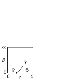
   Figure 1: A schematic flow diagram deduced from a strong coupling expansion.

   

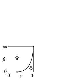
   Figure 2: A possible extrapolation. The critical line ends at $(r,\beta)=(1,\infty)$.

   

   Figure 3: A possible extrapolation. The critical line ends somewhere on the line $r=1$.

   

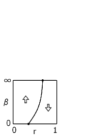
   Figure 4: A possible extrapolation. The critical line ends somewhere on the line $\beta=\infty$.

   However, a simple weak-coupling calculation for $SU(2)$ shows that by one MMK transformation the effective coupling changes from $\beta$ to $\beta/r\ (>\beta)$. So the flow goes toward the weak couling limit for sufficiently large $\beta\gg 1$ and for any fixed $r<1$, which implies that we can exclude the possibility of fig.4. At present we do not know which of fig.4 or 4 is the correct one.

   But does such a difference matter?

   Yes, it strongly does. For illustration, let us believe fig.4. Then for any $r<1$ and large initial coupling $\beta\gg 1$, the flow would go to the weak coupling limit: $\displaystyle\lim_{n\to\infty}c_{j}(n)=1$. In such a case, the existence of $t(1)=t^{*}$ no longer guarantees quark confinement, since the strong coupling cluster expansion is inapplicable to the r.h.s. of (38). Thus the alleged proof completely fails for $\beta\gg 1$ in the situation of fig.4. In contrast, if fig.4 were the case, then for arbitrary initial $\beta$ we can always find an appropriate value of $r<1$ for which the flow still goes to the strong coupling limit, hence the proof is valid (except for the step of showing the existence of $t^{*}$).

   These considerations clearly show the importance of ascertaining the qualitative flow of coupling under the MMK transformation, but Tomboulis in ref.[15] simply asserts that $r<1$ can be chosen very close to 1 so that the flow to the strong coupling limit is not destroyed. (This amounts to assuming the situation of fig.4 implicitly.) However he gave neither analytical nor numerical evidence of his claim. This constitutes the second incomplete point of the proof.

   As an aside we note that it is not mandatory to use a fixed value of $r$ throughout a flow. For example, for a fixed initial coupling $\beta$, we are allowed to choose different values of $r$ for every step of decimation, so that $\{c_{j}(1)\}_{j}$ is calculated from $\{c_{j}(0)\}_{j}$ via (24) with $r=r_{1}<1$, $\{c_{j}(2)\}_{j}$ is calculated from $\{c_{j}(1)\}_{j}$ via (24) with $r=r_{2}<1$, … and so on. However we can verify it does not make much difference: indeed, if fig.4 is true and $\beta\gg 1$, the flow would inevitably go to the weak coupling limit ($\beta\to\infty$) regardless of whatever values we choose for $\{r_{i}\}_{i}$. It is still vital even under such a looser condition to find out the flow diagram of the MMK transformation.

3. The third criticism is more indirect than the two given above: since the compact $U(1)$ lattice gauge theory in four dimensions has a deconfined phase at weak coupling [23], the proposed proof must fail for the abelian theory, but which specific step of the proof fails?

   Logically speaking, there are only two ways to reply:

   1. “The difference between abelian and nonabelian theories does not emerge until we complete the proof of the existence of $t^{*}=t(1)$. Such a proof, if any, is expected to become rather involved, since the delicate difference between abelian and nonabelian theories on the lattice has to be accounted for.”

   2. “The flow of the effective coupling under the MMK transformation is significantly different for abelian and nonabelian theories. Fig.4 applies to the abelian case, while fig.4 applies to the nonabelian case, which implies that the proof surely fails for the abelian case. ”

   Much more work will be needed to determine which scenario is the right one.

4. The fourth point concerns the necessity of the parameter $r$ itself. Before in this article we briefly explained the reason why $r$ was introduced; it was to avoid $\displaystyle\frac{\,dh(\alpha^{(n)}_{\Lambda,h}(t),t)\,^{\mathstrut}}{\,dt\,_{\mathstrut}}\to 0$ as $|\Lambda|\to\infty$. However it was not shown in ref.[15] whether such an undesirable behavior actually occurs or not. It is easy to see that it will occur if and only if the original MK transformation ($r=1$) becomes exact in the thermodynamic limit insofar as the free energy density is concerned. However, considering that the MK transformation is an approximate decimation scheme which bunches $b$ parallel adjacent plaquettes into one, it seems more plausible that the MK transformation can be exact at zero coupling ($\beta=\infty$) alone; in such a case, any fluctuation disappears and the actions of adjacent plaquettes will have equal expectation values, thus making the bunching an exact procedure.

   So the author’s guess is that $r$ is unnecessary to establish theorem 3. If it were the case, we could dispense with any modification of the original MK transformation. It is a sad news for the whole proof, however, since the abelian and nonabelian theories qualitatively behave in the same way under the original MK transformation (recall that the effective coupling flows to the strong coupling limit under the iterated MK transformations regardless of the initial coupling whether the gauge group is abelian or nonabelian) and so the difference between abelian and nonabelian theories has to be explained within the proof of the existence of $t^{*}=t(1)$, implying that much remains to be done to prove the quark confinement.

   Though our guess is by no means conclusive, this point deserves further study.

These are the main aspects of the alleged proof which are not clear enough to the author. The fact is that, the ultimate goal of ref.[15] (giving a proof of quark confinement) is not yet achieved, and instead, what has already been actually proved with a satisfactory rigor is theorem 3. One purpose of this paper is to point out that it can be derived in a far simpler way, bypassing the complicated discussion on the MMK transformation at all.

A.2 Discussion

First we state and prove a theorem. Its intriguing implication will be described afterwards in relation to our previous analyses.

Theorem 4.

Let the gauge group (denoted by $G$) a compact and connected Lie group. With $r\equiv 1-\displaystyle\frac{\,1\,^{\mathstrut}}{\,b^{2}\,_{\mathstrut}}$, the coefficients $\{c_{j}(n)\}$ defined by (24) converge to the strong-coupling limit (i.e. $\displaystyle\lim_{n\to\infty}c_{j}(n)=0$) if $b\in{\mathbf{N}}$ is chosen sufficiently large, depending on the initial coupling $\{c_{j}(0)\}$.

Proof.

Let us define a functional space

$$\mathfrak{F}\equiv\{f\in C^{2}(G)\,\big{|}\,f>0,\,f({\mathbf{1}})=1\}$$ (40)

(${\mathbf{1}}$ is the unit element of $G$ and $C^{2}(G)$ is a set of continuously twice-differentiable functions on $G$) and a map $T:\mathfrak{F}\to\mathfrak{F}$ by

$$Tf(U)\equiv\displaystyle\frac{\,(f^{q})^{*s}(U)\,^{\mathstrut}}{\,(f^{q})^{*s}({\mathbf{1}})\,_{\mathstrut}},\ \ \ \ \ s,q\in{\mathbf{N}},\ s\geq 2,\ U\in G,\ f\in\mathfrak{F}.$$ (41)

Here $(\dots)^{*s}$ denotes an $s$-fold convolution. (41) is nothing but the original MK transformation ($r=1$); if we put $q=s=b^{2}$, (41) reduces to (24) and (25) with $r=1$ except for an irrelevant normalization factor. Note that $Tf$ is a class function over $G$ if $f$ is. Let $V_{f}(U)\equiv-\log f(U)$.

Introducing a specific functional $W[f]$ (whose explicit form is not necessary for our purpose), $\rm{M\ddot{u}ller}$ and Schiemann [22] proved the following inequalities which hold for ${}^{\forall}f\in\mathfrak{F}$:

$$(V_{f})_{\mathrm{max}}-(V_{f})_{\mathrm{min}}\leq\displaystyle\frac{\,1\,^{\mathstrut}}{\,2\,_{\mathstrut}}W[f],$$ (42)

$$W[Tf]\leq\displaystyle\frac{\,q\,^{\mathstrut}}{\,s\,_{\mathstrut}}(1-e^{-W[f]})W[f],$$ (43)

where $(V_{f})_{\mathrm{max}}$ ($(V_{f})_{\mathrm{min}}$) is the maximum (minimum) value of $V_{f}$ over $G$. (We would like to emphasize that the definition of $W[f]$ and the property (42) are entirely independent of the map $T$.) We refrain from reproducing their proof here. Instead we would like to note one of its major consequences. If $\displaystyle\frac{\,q\,^{\mathstrut}}{\,s\,_{\mathstrut}}\leq 1$ holds, (43) implies that $W[T^{n}f]\leq W[f]$ for ${}^{\forall}n\in\mathbf{N}$. From this and (42), (43) we obtain

$$\hskip 50.0pt0\leq W[T^{n}f]\leq\big{(}1-e^{-W[f]}\big{)}^{n}W[f],\ \ \ \ \ \ \ \ {{}^{\forall}n\in\mathbf{N}}.$$ (44)

$$\therefore\ \displaystyle\lim_{n\to\infty}W[T^{n}f]=0.$$ (45)

(42) and (45) imply that $\displaystyle\lim_{n\to\infty}V_{T^{n}f}$ is a constant function on $G$ and so is $\displaystyle\lim_{n\to\infty}T^{n}f$. Thus, if $f$ is a class function on $G$, every coefficient in the character expansion of $T^{n}f$ would tend to $0$ as $n\to\infty$ except for a constant term. This completes the proof of the convergence of the original MK transformation.

Let us then prove theorem 4. If we introduce $r\in(0,1)$, $s$ changes from $b^{2}$ to $b^{2}r$ while $q=b^{2}$ remains unchanged. However we have to be careful at this point: $b^{2}r$ is not integral in general while (42) and (43) have been proved only for an integral $s$. Let us choose, for example, $r=1-\displaystyle\frac{\,1\,^{\mathstrut}}{\,b^{2}\,_{\mathstrut}}$ so that $b^{2}r\in{\mathbf{N}}$. Then (43) yields

$$W[Tf]\leq\displaystyle\frac{\,1-e^{-W[f]}\,{}^{\mathstrut}}{\,r\,_{\mathstrut}}W[f].$$ (46)

Let us take $b$ so large that $\displaystyle\frac{\,1-e^{-W[f]}\,{}^{\mathstrut}}{\,r\,_{\mathstrut}}<1$. Then we have $W[T^{n}f]\leq W[f]$ also in this case. It is straightforward to derive

$$\hskip 55.0pt0\leq W[T^{n}f]\leq\left(\displaystyle\frac{\,1-e^{-W[f]}\,{}^{\mathstrut}}{\,r\,_{\mathstrut}}\right)^{n}W[f],\ \ \ \ \ \ \ \ {{}^{\forall}n\in\mathbf{N}}.$$ (47)

$$\therefore\ \displaystyle\lim_{n\to\infty}W[T^{n}f]=0.$$ (48)

This completes the proof of theorem 4. ∎

The most important feature of theorem 4 is that it holds both for abelian and for nonabelian theories. In the third discussion of the previous section, we pointed out the possibility that the flow of the effective coupling under the MMK transformation for abelian theories might be significantly different from that of nonabelian theories making consistent the alleged proof of quark confinement for $SU(2)$ and the deconfinement phase of the $U(1)$ theory mutually. However, surprisingly, theorem 4 has made it clear that for any initial coupling we can choose $r$ smaller than 1 without messing the renormalization group flow toward the strong coupling limit, both for abelian and for nonabelian theories. The price we have to pay is just to choose an appropriate value of $b\in\mathbf{N}$, which does the proof no harm, since none of the steps of the proof explicitly depends on the choice of $b$. Thus, qualitatively speaking, there are only two scenarios possible:

1. “ We should prove the existence of $t^{*}=t(1)$ in such a way that does not permit to choose $b\gg 1$ for $\beta\gg 1$.”

2. “ We should prove the existence of $t^{*}=t(1)$ in such a way that incorporates the nonperturbative dynamics of the theory well enough to reveal the delicate difference between abelian and nonabelian theories on the lattice.”

If the first scenario were to be realized, then the prescription learned from theorem 4 (to vary $b$ depending on the initial coupling) is not implementable and we again face with the need to understand the flow diagram of the MMK transformation. But the first scenario looks quite bizarre in the sense that any argument that is valid for, say, $b\leq 3$ but becomes completely invalid for $b>4$ seems to be unphysical.

Thus we regard the second scenario as the one to be pursued. Since it essentially says that the proposed proof in its present form is unable to tell the abelian from the nonabelian theory at all, we are inclined to conclude that the proposed proof has made little or no progress compared with the original MK transformation.

We would like to summarize our comments on the present situation. The main tool exploited in ref.[15] is the Migdal-Kadanoff transformation (with a modification). It is an approximation; it is not the genuine, exact renormalization group transformation of the Yang-Mills theory on the lattice. Therefore if one is to make use of it to say something exact about the real Yang-Mills theory, it could be done only after exactly understanding the relation between the Migdal-Kadanoff approximation and the Yang-Mills theory. However it does not seem to be done in ref.[15]; although a rigorous inequality is proved concerning their relation, it is generally impossible to obtain an exact value via an inequality (an inequality is not an equality). Suppose we want to solve the equation $f(x)=0$ with the knowledge that the solution surely exists in the range $2<x<3$. By interpolation it can be rewritten as $x=2c+3(1-c)$ for some $0<c<1$. It is in the disguise of an equality, but we know that no new information is obtained through an interpolation alone. Such interpolations are repeatedly used throughout ref.[15], but obviously they give us no new information about confinement. Essentially this is the very reason the approach of ref.[15] is unsuccessful and looks hard to remedy.

References

- [1] R. Alkofer and J. Greensite, J. Phys. G: Nucl. Part. Phys. 34, S3 (2007).
- [2] Y. Nambu, Phys. Rev. D10, 4262 (1974); G. ’t Hooft, High Energy Physics EPS Int. Conference, Palermo 1975, ed. A. Zichichi; S. Mandelstam, Phys. Rep. 23, 245 (1976).
- [3] G. ’t Hooft, Nucl. Phys. B138, 1 (1978); ibid. B153, 141 (1979).
- [4] J. Greensite, Progr. Part. Nucl. Phys. 51, 1 (2003) [arXiv:hep-lat/0301023] and references therein.
- [5] A. M. Polyakov, Nucl. Phys. B120, 429 (1977); J. Glimm and A. Jaffe, Phys. Lett. B66, 67 (1977); J. , Phys. Lett. B83, 195 (1979); G. Mack, Commun. Math. Phys. 65, 91 (1979); D. J. Gross and E. Witten, Phys. Rev. D21, 446 (1980); M. and G. Mack, Commun. Math. Phys. 82, 545 (1982); N. Seiberg and E. Witten, Nucl. Phys. B426, 19 (1994).
- [6] T. Yoneya, Nucl. Phys. B144, 195 (1978).
- [7] G. Mack and V. B. Petkova, Annals Phys. 123, 442 (1979); ibid. 125, 117 (1980).
- [8] G. S. Bali, Phys. Rept. 343, 1 (2001) [arXiv:hep-ph/0001312v2] and references therein.
- [9] J. M. Cornwall, Nucl. Phys. B157, 392 (1979).
- [10] L. Del Debbio, M. Fabor, J. Greensite and S. Olejnik, Phys. Rev. D55, 2298 (1997) [arXiv:hep-lat/9610005].
- [11] P. de Forcrand and M. D’Elia, Phys. Rev. Lett. 82, 4582 (1999) [arXiv:hep-lat/9901020v2].
- [12] E. T. Tomboulis and L. G. Yaffe, Commun. Math. Phys. 100, 313 (1985).
- [13] G. Nucl. Phys. B180[FS2], 23 (1981).
- [14] T. and E. T. Tomboulis, Phys. Rev. Lett. 85, 704 (2000) [arXiv:hep-lat/0002004].
- [15] E. T. Tomboulis, arXiv:0707.2179v1[hep-th].
- [16] K. R. Ito and E. Seiler, arXiv:0803.3019[hep-th].
- [17] T. Kanazawa, arXiv:0808.3442[math-ph].
- [18] R. and D. Preiss, Commun. Math. Phys. 103, 491 (1986).
- [19] A. A. Migdal, ZhETF (USSR) 69, 810; 1457 (1975) [JETP (Sov. Phys.) 42, 413; 743 (1976)].
- [20] L. P. Kadanoff, Ann. of Phys. 100, 359 (1976); Rev. Mod. Phys. 49, 267(1977).
- [21] K. R. Ito, Phys. Rev. Lett. 55, 558 (1985).
- [22] V. F. and J. Schiemann, Lett. Math. Phys. 15, 289 (1988).
- [23] A. H. Guth, Phys. Rev. D21, 2291 (1980); J. and T. Spencer, Commun. Math. Phys. 83, 411 (1982).