Evolution of neutron stars with toroidal magnetic fields: Axisymmetric simulation in full general relativity

Abstract

We study the stability of neutron stars with toroidal magnetic fields by magnetohydrodynamic simulation in full general relativity under assumption of axial symmetry. Nonrotating and rigidly rotating neutron stars are prepared for a variety of magnetic field configuration. For modeling the neutron stars, the polytropic equation of state with the adiabatic index $\Gamma=2$ is used for simplicity. It is found that nonrotating neutron stars are dynamically unstable for the case that toroidal magnetic field strength varies $\propto\varpi^{2k-1}$ with $k\geq 2$ (here $\varpi$ is the cylindrical radius), whereas for $k=1$ the neutron stars are stable. After the onset of the instability, unstable modes grow approximately in the Alfvén time scale and, as a result, a convective motion is excited to change the magnetic field profile until a new state, which is stable against axisymmetric perturbation, is reached. We also find that rotation plays a role in stabilization, although the instability still sets in in the Alfvén time scale when the ratio of magnetic energy to rotational kinetic energy is larger than a critical value $\sim 0.2$. Implication for the evolution of magnetized protoneutron stars is discussed.

I Introduction

Neutron stars observed in nature are magnetized with the typical magnetic field strength $\sim 10^{11}$–$10^{13}$ G Lyne . The field strength is often much larger than the canonical value as $\sim 10^{15}$ G for a special class of the neutron stars such as magnetars WD . The field strength at the birth of neutron stars may be also much larger than the canonical value, because in the supernova gravitational collapse, rapid and differential rotation of the collapsing core could amplify the magnetic field. In the presence of a radial magnetic field $B^{\varpi}$, the toroidal field $B^{T}$ is amplified by winding in the presence of differential rotation, and the field strength increases with time approximately according to (see, e.g., AHM ; SLSS )

$$B^{T} \sim B^{\varpi}\Omega t$$ (1)

$$= 10^{15}\biggl{(}{B^{\varpi}\over 10^{12}~{}{\rm G}}\biggr{)}\biggl{(}{\Omega\over 10^{2}~{}{\rm rad/s}}\biggr{)}\biggl{(}{t\over 10~{}{\rm s}}\biggr{)}~{}{\rm G},$$

where we adopt the typical magnitude of the angular velocity and the typical cooling time of the protoneutron star for $\Omega$ and $t$. The large field strength of the magnetars may be generated by such process and subsequently be confined inside the neutron star for thousands of years Spruit . This suggests that even for the normal pulsar, the toroidal field strength inside the neutron star may be much larger than the canonical value. Thus, strongly magnetized neutron stars may be common in nature. In particular, the toroidal field is likely to be much stronger than the poloidal fields inside neutron stars. In this paper, we focus on the effect of such strong toroidal magnetic fields for the dynamical evolution of neutron stars.

Stars with purely toroidal magnetic fields in a stably stratified structure are known to be unstable against the Tayler instability Tayler ; Acheson ; Tayler2 ; Spruit99 (see also Appendix A). According to a perturbative study in Tayler ; Acheson ; Tayler2 ; Spruit99 , the most unstable motions are driven by axisymmetric ($m=0$) and nonaxisymmetric $m=1$ modes with nearly horizontal displacement. The unstable modes are predicted to grow approximately on an Alfvén time scale. The Alfvén time scale of magnetized neutron stars are estimated to be very short as

$$\tau_{A} \sim {R\over v_{A}}$$ (2)

$$\sim 30\biggl{(}{R\over 10~{}{\rm km}}\biggr{)}\biggl{(}{\rho\over 10^{14}~{}{\rm g/cm^{3}}}\biggr{)}^{{1\over 2}}\biggl{(}{B^{T}\over 10^{15}~{}{\rm G}}\biggr{)}^{-1}~{}{\rm ms},$$

where $R$ and $\rho$ are characteristic radius and density of the neutron star, $v_{A}$ is the Alfvén speed, and we use $v_{A}=B^{T}/(4\pi\rho)^{1/2}$. The time scale for the growth of the Tayler instability is only by one order of magnitude longer than the dynamical time scale of neutron stars which is $\sim 1$ ms. Thus, the instability associated with the strong magnetic fields may affect even early evolution of the protoneutron star and, consequently, supernova explosion. However, perturbative studies do not clarify anything in the nonlinear evolution stage reached after a sufficient growth of the instability.

To understand roles of strong toroidal fields on the evolution of neutron stars and protoneutron stars, numerical simulation is probably the best approach. In this paper, we present our new numerical results obtained by general relativistic magnetohydrodynamic (GRMHD) simulation, for which our GRMHD code recently developed SS05 is used. We prepare neutron stars with purely toroidal magnetic fields in axisymmetric equilibria computed by a method described in KY . As a first step toward a deep understanding of the Tayler instability, we focus on the $m=0$ mode imposing axial symmetry. As shown in Spruit99 , neutron stars are unstable if certain condition is satisfied for the magnetic field profile and for the rotation rate. We confirm this fact in the present numerical simulation. In addition, we follow evolution of the unstable stars after the onset of the Tayler instability and show that associated with the growth of this instability, a convective motion is driven inside the neutron star. Then, the magnetic fields are redistributed and eventually their profile relaxes to a new state which is stable against axisymmetric perturbation.

The remainder of this paper is organized as follows. In Sec. II, we briefly review formulation and numerical methods for our GRMHD simulations. Section III presents numerical results for nonrotating and rotating neutron stars separately. Section IV is devoted to a summary and discussion about implication of the present results on the evolution of neutron stars. In Appendix A, we present a result of linear perturbative study for neutron stars of purely toroidal magnetic fields, which validates our numerical results qualitatively. Throughout this paper, we adopt geometrical units in which $G=1=c$, where $G$ and $c$ denote the gravitational constant and speed of light, respectively. Cartesian coordinates are denoted by $x^{k}=(x,y,z)$. The coordinates are oriented so that the symmetric axis is along the $z$-direction. We define the coordinate radius $r=\sqrt{x^{2}+y^{2}+z^{2}}$, cylindrical radius $\varpi=\sqrt{x^{2}+y^{2}}$, and azimuthal angle $\varphi=\tan^{-1}(y/x)$. Coordinate time is denoted by $t$. Greek indices $\mu,\nu,\cdots$ denote spacetime components, and small Latin indices $i,j,\cdots$ denote spatial components.

II Method for numerical simulation

II.1 Formulation and methods

The stability of magnetized neutron stars and the fate of unstable neutron stars are investigated by GRMHD simulation assuming that the ideal MHD condition holds. In this paper, we assume the axial symmetry and focus only on the Tayler instability against axisymmetric perturbation. The simulation is performed by a GRMHD code for which the details are described in SS05 . This code makes long-term numerical evolutions of relativistic magnetized neutron stars possible. It solves the Einstein-Maxwell-MHD system of coupled equations, both in axial symmetry and in 3+1 dimensions, without approximation. The code evolves the spacetime metric using the BSSN formulation BSSN ; we evolve the conformal three metric $\tilde{\gamma}_{ij}=\gamma^{-1/3}\gamma_{ij}$, a conformal factor $\phi=\ln(\gamma)/12$, a tracefree extrinsic curvature $\tilde{A}_{ij}=e^{-4\phi}(K_{ij}-\gamma_{ij}K_{k}^{~{}k}/3)$, trace of the extrinsic curvature $K_{k}^{~{}k}$, and an auxiliary three variable $F_{i}=\sum_{j}\partial_{j}\tilde{\gamma}_{ij}$. Here, $\gamma_{ij}$ is the three-metric and $\gamma={\rm det}(\gamma_{ij})$. For axisymmetric simulation, the Cartoon method is employed alcu ; S03 : Namely, the Einstein equation is solved in the Cartesian coordinates imposing an axisymmetric boundary condition and the hydrodynamic equation is in the cylindrical coordinates.

As in previous axisymmetric simulations (e.g., S2d ; SS05 ), the following dynamical gauge condition is employed

$$\partial_{t}\alpha=-\alpha K_{k}^{~{}k},$$ (3)

$$\partial_{t}\beta^{i}=\tilde{\gamma}^{ij}(F_{j}+\Delta t\partial_{t}F_{j}),$$ (4)

where $\alpha$ is the lapse function, $\beta^{i}$ the shift vector, and $\Delta t$ time step in numerical computation.

A conservative shock-capturing scheme is employed to integrate the GRMHD equations. Specifically we use a high-resolution central scheme KT ; lucas with the third-order piece-wise parabolic interpolation and with a steep min-mod limiter in which the limiter parameter $b$ is set to be 2.5 (see appendix A of S03 ). Multiple tests have been performed with these codes, including MHD shocks, MHD wave propagation, magnetized Bondi accretion, and magnetized accretion onto a neutron star SS05 . This code has been already applied to the evolution of magnetized hypermassive neutron stars to a black hole DLSSS ; DLSSS2 and to supernova gravitational collapse of strongly magnetized and rotating core SLSS , and derived reliable numerical results.

In the present paper, we initially give a purely toroidal magnetic field. In such a case, poloidal magnetic fields are never generated in the axisymmetric spacetime. Thus, we only solve the toroidal field component.

As initial conditions for the numerical simulation, we prepare magnetized neutron stars in equilibrium KY . For computing the equilibrium, we give the polytropic equation of state as

$$P=\kappa\rho^{\Gamma},$$ (5)

where $P$, $\rho$, $\kappa$, and $\Gamma$ are the pressure, rest-mass density, polytropic constant, and adiabatic constant. In this work, we choose $\Gamma=2$. Because $\kappa$ is arbitrarily chosen or else completely scaled out of the problem, we adopt the units of $\kappa=1$ in the following (i.e., the units of $c=G=\kappa=1$).

In numerical simulation, we adopt the $\Gamma$-law equation of state

$$P=(\Gamma-1)\rho\varepsilon,$$ (6)

where $\varepsilon$ is the specific internal thermal energy.

Table 1: List of characteristic quantities for neutron stars with toroidal magnetic fields. Value of $k$, central density, $\rho_{c}$, baryon rest mass, $M_{*}$, ADM mass, $M$, ratio of equatorial circumferential radius $R$ to $M$, ratio of the rotational kinetic energy to the gravitational potential energy, $T_{\rm rot}/W$, ratio of the internal thermal energy to $W$, $E_{\rm int}/W$, ratio of the electromagnetic energy to $W$, $E_{\rm EM}/W$ , non-dimensional angular momentum parameter, $J/M^{2}$, central value of the lapse function, $\alpha_{c}$, angular velocity, $\Omega$, and Alfvén time scale defined by Eq. (21). All the quantities are shown in units of $c=G=\kappa=1$. For models AXY, BXY, and CXY, $k=1$, 2, and 3, respectively. “X” denotes the value of $10\rho_{c}$ and “Y”(=H, M, L) denotes the relative strength of the magnetic field. Models RAXY and RBXY denote rapidly rotating neutron stars (meaning of A, B, X, and Y is the same as above). Models MBXy denote moderately rapidly rotating neutron stars. Models EBXy and SBXy denote rotating models with very strong and strong magnetic fields, respectively. “y” approximately denotes $100T/W$. In the last column, the stability determined by the numerical simulation is described.

Model	$k$	$\rho_{c}$	$M_{*}$	$M$	$R/M$	$T_{\rm rot}/W$	$E_{\rm int}/W$	$E_{\rm EM}/W$	$J/M^{2}$	$\alpha_{c}$	$\Omega$	$\bar{\tau}_{A}/M$	Stable ?
A3H	1	0.3000	0.1793	0.1637	4.821	0	0.5858	0.0146	0	0.4786	0	67.8	Yes
A3L	1	0.3000	0.1798	0.1637	4.749	0	0.5931	$9.8\times 10^{-4}$	0	0.4756	0	256	Yes
A2H	1	0.2000	0.1715	0.1574	5.599	0	0.5148	0.0135	0	0.5732	0	89.6	Yes
B3H	2	0.3000	0.1794	0.1637	4.783	0	0.5880	0.0122	0	0.4772	0	73.4	No
B3M	2	0.3000	0.1797	0.1637	4.750	0	0.5927	$2.05\times 10^{-3}$	0	0.4757	0	177	No
B3L	2	0.3000	0.1798	0.1637	4.747	0	0.5932	$9.3\times 10^{-4}$	0	0.4755	0	263	No
B2H	2	0.2000	0.1714	0.1573	5.543	0	0.5168	0.0108	0	0.5715	0	98.5	No
B2M	2	0.2000	0.1717	0.1573	5.516	0	0.5201	$3.11\times 10^{-3}$	0	0.5703	0	182	No
B2L	2	0.2000	0.1717	0.1574	5.505	0	0.5210	$1.16\times 10^{-3}$	0	0.5700	0	297	No
C3L	3	0.3000	0.1798	0.1638	4.747	0	0.5931	$1.16\times 10^{-3}$	0	0.4755	0	236	No
C2H	3	0.2000	0.1714	0.1573	5.537	0	0.5169	0.0108	0	0.5713	0	98.5	No
RA2H	1	0.2000	0.1986	0.1821	6.732	0.0808	0.4555	0.0145	0.5667	0.5383	0.3159	99.5	Yes
RA2L	1	0.2000	0.2021	0.1848	6.491	0.0866	0.4577	$1.78\times 10^{-3}$	0.5894	0.5318	0.3271	272	Yes
RB2S	2	0.2000	0.1981	0.1817	6.283	0.0796	0.4559	0.0176	0.5614	0.5382	0.3144	84.4	No
RB2H	2	0.2000	0.2002	0.1835	6.594	0.0839	0.4549	0.0126	0.5783	0.5352	0.3211	104	Yes
RB2L	2	0.2000	0.2023	0.1850	6.478	0.0869	0.4575	$1.78\times 10^{-3}$	0.5906	0.5315	0.3276	271	Yes
MB2H	2	0.2000	0.1908	0.1751	5.863	0.0611	0.4708	0.0163	0.4870	0.5460	0.2852	82.6	No
MB2M	2	0.2000	0.1906	0.1747	5.797	0.0597	0.4744	0.0108	0.4817	0.5456	0.2832	99.9	No
MB2L	2	0.2000	0.1903	0.1743	5.738	0.0581	0.4780	$5.66\times 10^{-3}$	0.4758	0.5453	0.2809	137	Yes
MB2L’	2	0.2000	0.1856	0.1700	5.649	0.0447	0.4882	$4.66\times 10^{-3}$	0.4151	0.5512	0.2512	149	Yes
EB27	2	0.200	0.1915	0.1765	6.251	0.0659	0.4550	0.0427	0.5040	0.5492	0.2886	54.8	No
EB25	2	0.200	0.1858	0.1713	5.995	0.0502	0.4667	0.0433	0.4353	0.5559	0.2592	52.6	No
EB23	2	0.2000	0.1793	0.1653	5.798	0.0302	0.4833	0.0392	0.3343	0.5635	0.2078	53.9	No
EB21	2	0.2000	0.1745	0.1610	5.744	0.0144	0.4922	0.0443	0.2286	0.5708	0.1465	50.6	No
SB24	2	0.2000	0.1845	0.1692	5.702	0.0430	0.4854	0.0137	0.4052	0.5536	0.2459	88.0	No
SB23	2	0.2000	0.1805	0.1656	5.629	0.0305	0.4955	0.0111	0.3400	0.5586	0.2109	97.2	No
SB21	2	0.2000	0.1744	0.1601	5.572	0.0108	0.5091	0.0116	0.2005	0.5671	0.1286	95.1	No

II.2 Diagnostics

We monitor the total baryon rest mass $M_{*}$, ADM (Arnowitt-Deser-Misner) mass $M$, and angular momentum $J$, which are computed, in axial symmetry, by

$$M_{*}=\int\rho u^{t}\sqrt{-g}d^{3}x,$$ (7)

$$M=\int\rho_{\rm ADM}\sqrt{\gamma}d^{3}x,$$ (8)

$$J=\int\rho hu^{t}u_{\varphi}\sqrt{-g}d^{3}x,$$ (9)

where $u^{\mu}$ is the four velocity, $g$ is the determinant of the spacetime metric, $h$ is the specific enthalpy ($h=1+\varepsilon+P/\rho$), and

$$\rho_{\rm ADM}=[\rho h(\alpha u^{t})^{2}-P]e^{-\phi}$$

$$~{}~{}~{}~{}~{}~{}~{}~{}+{e^{-\phi}\over 16\pi}\biggl{[}K_{ij}K^{ij}-(K_{k}^{~{}k})^{2}-\tilde{R}e^{-4\phi}\biggr{]}.$$ (10)

Here, $\tilde{R}$ is the Ricci scalar with respect to $\tilde{\gamma}_{ij}$. Hereafter, initial ADM mass is denoted by $M_{0}$.

In addition to the above quantities, we monitor the internal thermal energy $E_{\rm int}$, rotational kinetic energy $T_{\rm rot}$, total kinetic energy $T_{\rm kin}$, and electromagnetic energy $E_{\rm EM}$, written by

$$E_{\rm int} = \int\rho u^{t}\varepsilon\sqrt{-g}d^{3}x,$$ (11)

$$T_{\rm rot} = {1\over 2}\int\rho hu^{t}u_{\varphi}\Omega\sqrt{-g}d^{3}x,$$ (12)

$$T_{\rm kin} = {1\over 2}\int\rho hu^{t}u_{i}v^{i}\sqrt{-g}d^{3}x,$$ (13)

$$E_{\rm EM} = {1\over 2}\int b^{2}u^{t}\sqrt{-g}d^{3}x,$$ (14)

where $b^{2}=b^{\mu}b_{\mu}$, $b^{\mu}$ is a magnetic vector in the frame comoving with fluid elements (e.g., SS05 ), and $v^{i}=u^{i}/u^{t}$. In this paper, magnetic field strength is defined by $\sqrt{4\pi b^{2}}$. We note that $E_{\rm EM}$ is defined originally by

$$E_{\rm EM}=\int T_{\rm EM}^{\mu\nu}n_{\mu}u_{\nu}\sqrt{\gamma}d^{3}x,$$ (15)

where $T_{\rm EM}^{\mu\nu}$ is the electromagnetic part of the energy momentum tensor and $n^{\mu}$ is the hypersurface normal, and hence, the definition is different from that in DLSSS2 . This definition is based on mimicking the definition of $E_{\rm int}$, which is

$$E_{\rm int}=\int T_{\rm hydro}^{\mu\nu}n_{\mu}u_{\nu}\sqrt{\gamma}d^{3}x-M_{*},$$ (16)

where $T_{\rm hydro}^{\mu\nu}(=\rho hu^{\mu}u^{\nu}+Pg^{\mu\nu})$ is the non-electromagnetic part of the energy momentum tensor.

Once each energy component is obtained, gravitational potential energy is defined by

$$W=M_{*}+E_{\rm int}+E_{\rm EM}+T_{\rm kin}-M.$$ (17)

The Alfvén speed in relativity is defined by

$$v_{A}=\sqrt{{b^{2}\over\rho h+b^{2}}}.$$ (18)

Associated Alfvén time scale is

$$\tau_{A}={L\over v_{A}},$$ (19)

where $L$ is a characteristic length scale and in the present context, it is approximately equal to stellar radius. Usually, the Alfvén time scale denotes a characteristic time during which Alfvén waves propagate for the characteristic length scale. In the present case, we assume the axial symmetry and presence of purely toroidal magnetic field, and hence, Alfvén waves play no role. Nevertheless, a dynamical instability analyzed in this paper grows in the time scale of order $\tau_{A}$. For this reason, we here define an averaged Alfvén time scale from global quantities as

$$\bar{v}_{A}\equiv\Biggl{[}{\displaystyle\int b^{2}u^{t}\sqrt{-g}d^{3}x\over\displaystyle\int(\rho h+b^{2})u^{t}\sqrt{-g}d^{3}x}\Biggr{]}^{{1\over 2}}$$

$$~{}~{}~{}~{}=\sqrt{2E_{\rm EM}\over M_{*}+\Gamma E_{\rm int}+2E_{\rm EM}},$$ (20)

where we use the relation $h=1+\Gamma\varepsilon$ which holds in the $\Gamma$-law equation of state. Then, we define averaged Alfvén time scale as

$$\bar{\tau}_{A}={R\over\bar{v}_{A}},$$ (21)

where $R$ is equatorial stellar radius.

II.3 Initial condition

We prepare a variety of neutron stars in equilibrium changing the compactness, profile and strength of toroidal magnetic fields, and rotational kinetic energy. The initial conditions are derived in the same method as that described in KY . In the present case, we give the toroidal magnetic field according to the relation

$$b_{\varphi}=B_{0}u^{t}(\rho h\alpha^{2}\gamma_{\varphi\varphi})^{k},$$ (22)

where $k$ and $B_{0}$ are constants which determine the field profile and field strength, respectively. Because of the regularity condition along the symmetric axis, $k$ has to be a positive integer. $\gamma_{\varphi\varphi}$ is the $\varphi\varphi$ component of $\gamma_{ij}$ and approximately proportional to $\varpi^{2}$ near the symmetric axis. Because $b_{\varphi}$ is a function of $\rho$, the magnetic field is confined inside the neutron star.

In this work, we choose $k=1$, 2, and 3. Because $b_{\varphi}$ is proportional to $\varpi^{2k}$ near the symmetric axis, the toroidal field strength defined by $B^{T}\equiv b_{\varphi}\gamma_{\varphi\varphi}^{-1/2}/\sqrt{4\pi}$ is proportional to $\varpi^{2k-1}$. Namely, for small values of $k$, the fields are confined near the symmetric axis. References Tayler ; Acheson ; Tayler2 ; Spruit (and also Appendix A) predict that stars with $k=1$ are stable against axisymmetric perturbation, whereas those with $k\geq 2$ are unstable, although rotation could stabilize the unstable mode.

Several key quantities which characterize the magnetized neutron stars are listed in Table I. $B_{0}$ is chosen so as to get $10^{-3}\mathrel{\raise 1.29167pt\hbox{$<$}\mkern-14.0mu\lower 2.58334pt\hbox{$\sim$}}E_{\rm EM}/W\mathrel{\raise 1.29167pt\hbox{$<$}\mkern-14.0mu\lower 2.58334pt\hbox{$\sim$}}4\times 10^{-2}$. For typical neutron stars of mass $\sim 1.4M_{\odot}$, $W\sim 6\times 10^{53}$ ergs. The electromagnetic energy is approximately written as $E_{\rm EM}\sim(B^{T})^{2}R^{3}/3$, and hence, the magnetic field strength we consider here is extremely large as $10^{16}$–$10^{17}$ G for $R\approx 10$ km. Such choice is done simply to save computational time (note that the time scale for the growth of unstable modes is proportional to $(B^{T})^{-1}$; see below). In all the cases, the magnetic field is strong but not strong enough to modify the stellar structure significantly; e.g., for the nonrotating case, the shape of the neutron stars is approximately spherical.

Even from this extreme setting, we can derive a generic physical essence because scaling relation, associated with the magnetic field strength, holds for the evolution of the unstable neutron star. Namely, if the magnetic field strength becomes half, the growth time scale for the Tayler instability becomes approximately twice longer, although the qualitative properties about the evolution of the unstable star are essentially the same. Hence, the artificial choice of the large magnetic field is acceptable for deriving generic physical properties.

Compactness of the neutron stars is determined from the conditions that the central density, $\rho_{c}$, is 0.300 or 0.200 (in units of $\kappa=1$). We note that the maximum rest mass and gravitational mass of spherical neutron stars for $\Gamma=2$ are 0.1799 and 0.1637, and the corresponding central density is $\approx 0.318$. This implies that the nonrotating neutron stars with $\rho_{c}=0.300$ are close to the marginally stable point against gravitational collapse. Indeed, the rest mass and ADM mass for such models are close to the values of marginally stable stars (cf. Table I). We will show that our code can follow such extremely compact stars stably for a long time $\mathrel{\raise 1.29167pt\hbox{$>$}\mkern-14.0mu\lower 2.58334pt\hbox{$\sim$}}3000M_{0}$. By contrast, with $\rho_{c}=0.2$, the ratio of the stellar radius to the ADM mass becomes $\sim 5.5$ for the nonrotating neutron stars, which is a typical magnitude for neutron stars (for a hypothetical value of ADM mass $1.35M_{\odot}$, $R\approx 11$ km). Thus, in this paper, we consider very compact and reasonably compact neutron stars.

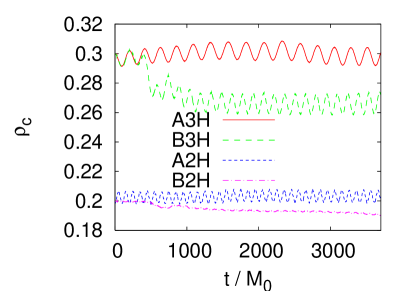
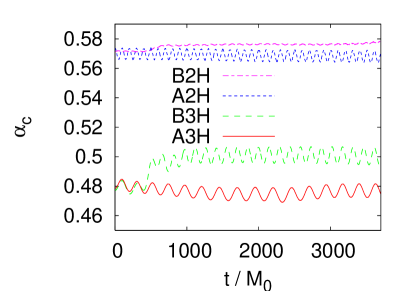
Figure 1: Evolution of central density and central value of the lapse function for models A3H (solid curves), B3H (long-dashed curves), A2H (dashed curves), and B2H (dashed-dotted curves). The units of time is initial ADM mass $M_{0}$.

We also prepare a variety of rotating neutron stars. In this paper, we focus only on rigidly rotating neutron stars with a moderate compactness; $\rho_{c}$ is fixed to be 0.200. For neutron stars with $\Gamma=2$ polytrope, the maximum ratio of rotational kinetic energy to gravitational potential energy, $T/W$, is $\sim 0.09$ for compact neutron stars with $R/M\approx 6$ CST . Here, at the maximum ratio, velocity at the equatorial surface of the star is equal to the Kepler velocity. Taking into account this fact, we prepare rotating stars with $0<T/W\mathrel{\raise 1.29167pt\hbox{$<$}\mkern-14.0mu\lower 2.58334pt\hbox{$\sim$}}0.09$. Specifically, we consider the following four sequences for studying dependence of stability on the rotation rate. First we consider rapidly rotating stars with $T/W=0.08$–0.09 or $T/W\approx 0.06$ and with $0.001\mathrel{\raise 1.29167pt\hbox{$<$}\mkern-14.0mu\lower 2.58334pt\hbox{$\sim$}}E_{\rm EM}/W\mathrel{\raise 1.29167pt\hbox{$<$}\mkern-14.0mu\lower 2.58334pt\hbox{$\sim$}}0.02$. The models in these categories are specified with models “R***” and “M***” (see the caption of Table I for the meaning of ***). In the third and fourth sequences, we approximately fix the values of $E_{\rm EM}/W$ as 0.04 and 0.01 but change the values of $T/W$ for a wide range. The models in these categories are specified with model “E***” and “S***”. By studying stability of these models, the dependence of stability criterion on $T/W$ and $E_{\rm EM}/W$ is clarified.

III Numerical simulation

III.1 Choosing the grid points and atmosphere

Numerical simulation was performed assuming the axial symmetry as well as the equatorial ($z=0$) plane symmetry. For covering computational domain, a nonuniform grid of the following grid structure is adopted for $\varpi$ and $z$:

$$x^{k}(i)=\left\{\begin{array}[]{ll}i\Delta x&1\leq i\leq N_{0}\\ i\Delta x+\xi\Delta i\Delta x&{}\\ ~{}\times\log[\cosh\{(i-N_{0})/\Delta i\}]&N_{0}<i\leq N.\end{array}\right.$$ (26)

Here, $x^{k}$ denotes $\varpi$ or $z$, $\Delta x$ is the grid spacing in the inner region, and $N_{0}$, $N$, $\Delta i$, and $\xi$ are constants which determine the grid structure of the outer part. In this grid setting, the inner domain with $0\leq\varpi\leq N_{0}\Delta x$ and $0\leq z\leq N_{0}\Delta x$ is covered by a uniform grid. Neutron stars are always covered in an inner region with $r<2N_{0}\Delta x/3$. $N_{0}$ is chosen to be 150 in this paper.

In the present simulation, mass ejection and expansion of stars do not occur in a remarkable manner, and hence, it is not necessary to resolve the outer region as accurately as the inner region where neutron stars are located. Thus, we prepare a rather large grid spacing for the outer region choosing $\Delta i=50$ and $\xi=10$. $N$ is set to be 240. In the following, we present results with this grid setting for all the cases. With this setting, outer boundaries along each axis are located at $L\approx 800\Delta x$ which is approximately equal to eight stellar radii ($\approx 8R$). These are large enough for excluding spurious effects from outer boundaries at least for $t\mathrel{\raise 1.29167pt\hbox{$<$}\mkern-14.0mu\lower 2.58334pt\hbox{$\sim$}}3000M_{0}$. Indeed, we performed a simulation for $N=220$ (i.e., $L\approx 600\Delta x$) while fixing other parameters for the grid structure, and found that results depend very weakly on $N$ (i.e., $L$; see Fig. 9). Nevertheless, for smaller values of $L$, the spurious effects coming from the outer boundaries are serious: For $L=300\Delta x\approx 3R$ and $600\Delta x\approx 6R$, the computation crashes eventually at $t\sim 2000M_{0}$ and $2700M_{0}$, respectively, in the chosen non uniform grid. However, note that the time at which computation crashes depends on the grid structure and for the uniform-grid case, the computation does not crash at $t=3500M_{0}$ even for $L=3R$.

For a convergence test, we performed additional simulations for model B3H, choosing uniform grid with $N=240$, 300, and 360. For each case, the equatorial radius of the neutron star is covered by 80, 100, and 120 grid points, respectively. Thus, for $N=300$, the grid resolution for the inner region with $i\leq 150$ is the same as that for the nonuniform grid. In these uniform grids, outer boundaries are located at three stellar radii ($L=3R$), but in these cases, the computation does not crash until $t=3500M_{0}$. A simulation was also performed in the nonuniform grid with $N=220$, in which $L\approx 600\Delta x$, as mentioned above. Comparison of the results for five simulations indicates that the resolution of our typical grid setting and location of outer boundaries are fine enough to derive quantitative results within 20–30% error (see the last two paragraphs of Sec. III.2.1).

Because any conservation scheme of hydrodynamics is unable to evolve a vacuum, we have to introduce an artificial atmosphere outside neutron stars. We initially assign a small rest-mass density of magnitude $\rho_{\rm at}=\rho_{\rm max}\times 10^{-8}$ where $\rho_{\rm max}$ is the maximum rest-mass density of the neutron star. With such choice, the total amount of the rest mass of the atmosphere is about $10^{-5}$ of the rest mass of the neutron star. Thus, the accretion of the atmosphere onto the neutron star plays a negligible role for their evolution.

III.2 Numerical results

III.2.1 Nonrotating case

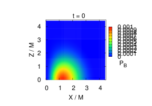
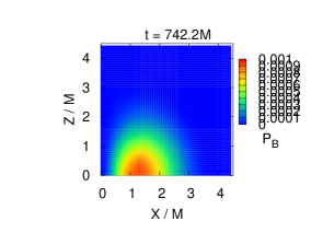
Figure 2: Snapshots for profiles of rest-mass density and magnetic pressure, $b^{2}/2$, for model A3H which is dynamical stable.

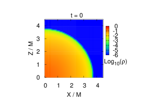
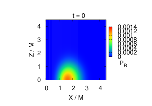
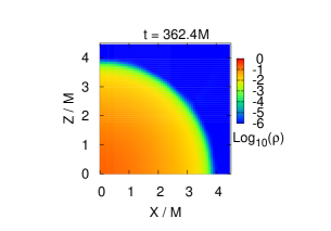
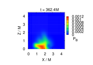
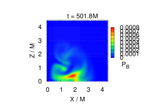
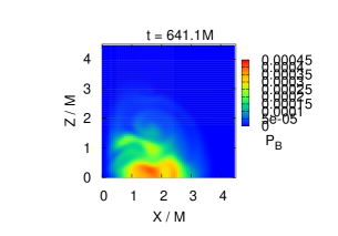
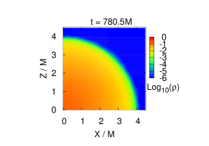
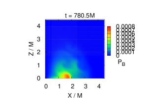
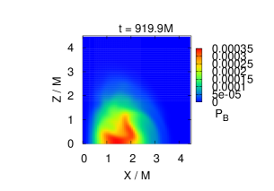
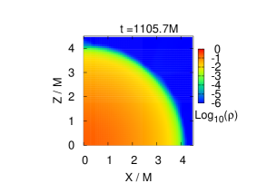
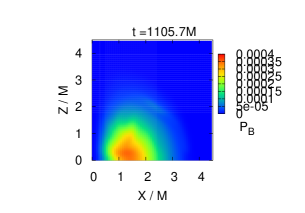
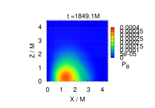
Figure 3: Snapshots for profiles of rest-mass density and magnetic pressure for model B3H.

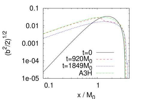
Figure 4: Profile of square root of magnetic pressure, $\sqrt{b^{2}/2}$, along $\varpi$-axis at selected time slices, $t/M_{0}=0$, 920, and 1849.1 for model B3H. For comparison, the profile for model A3H at $t=0$ is shown together.

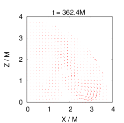
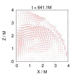
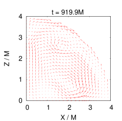
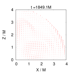
Figure 5: Snapshots of velocity fields for model B3H at selected time slices, $t/M_{0}=362.4$, 641.1, 919.9, and 1849.1 (cf. Fig. 3 for the magnetic field profile at the same time slices). For each time, the maximum velocity (the maximum value of $\sqrt{(v^{\varpi})^{2}+(v^{z})^{2}}$) is 0.039, 0.047, 0.041, and 0.037, respectively.

We performed numerical simulations for all the models listed in Table I. All the simulations stably proceeded for a sufficiently long time to more than $3000M_{0}$. For the case that unstable modes of MHD grow in the Alfvén time scale, the simulation time is long enough to determine the stability of each neutron star and to follow subsequent evolution after the onset of the instability for our chosen models.

By the numerical simulations, we find that all the models with $k=1$ are stable and the profiles of density and magnetic field do not change significantly during evolution. By contrast, all the nonrotating models with $k\geq 2$ are unstable irrespective of the magnetic field strength. In this case, the magnetic fields are redistributed, and as a result, a convective motion is excited inside the neutron star. The unstable stars slightly expand and the central density decreases (cf. Fig. 1). Eventually, the star relaxes to a new state which is stable against axisymmetric perturbations. These conclusions hold irrespective of the magnetic field strength and compactness of the neutron stars. In the following, we describe characteristic features for stable and unstable stars showing numerical results for specific models.

Figure 1 plots evolution of central density and central value of the lapse function for models A3H, B3H, A2H, and B2H. This illustrates that for models A3H and A2H, the neutron stars simply oscillate around their hypothetical equilibrium states. The oscillation is excited because the initial model deviates slightly from the true equilibrium. The oscillation amplitude is larger for $\rho_{c}=0.3$ than that for $\rho_{c}=0.2$. This reflects a fact that the neutron stars with $\rho_{c}=0.3$ are close to the marginally stable point against gravitational collapse, and a small perturbation induces a large deviation from the equilibrium state. In contrast to models A3H and A2H, for models B3H and B2H, the central density and lapse quickly change at $t\sim 500M_{0}$, implying that the stars expand. This is due to the fact that the profile of magnetic fields is modified during the evolution.

Figures 2 and 3 display snapshots for the profiles of density and magnetic pressure for models A3H and B3H at selected time slices. For model A3H in which the neutron star is stable, the profiles remain approximately static besides a slight oscillation. By contrast, model B3H is dynamically unstable against redistribution of magnetic fields: For $t\mathrel{\raise 1.29167pt\hbox{$<$}\mkern-14.0mu\lower 2.58334pt\hbox{$\sim$}}400M_{0}$, the profile of the magnetic pressure distribution gradually varies, and then, for $400\mathrel{\raise 1.29167pt\hbox{$<$}\mkern-14.0mu\lower 2.58334pt\hbox{$\sim$}}t/M_{0}\mathrel{\raise 1.29167pt\hbox{$<$}\mkern-14.0mu\lower 2.58334pt\hbox{$\sim$}}1000$, the magnetic fields are redistributed violently. As described in Appendix A, unstable modes grow near the equatorial plane as well as in a high latitude of $z\sim M_{0}$ and $\varpi\sim 2M_{0}$. For $t\mathrel{\raise 1.29167pt\hbox{$>$}\mkern-14.0mu\lower 2.58334pt\hbox{$\sim$}}1000M_{0}$, the profile approaches to a new state which is stable against axisymmetric perturbation. The maximum magnetic pressure decreases after the onset of the instability. As a result, the pinching effect by the toroidal magnetic fields are weaken. This is the reason that the star slightly expands and the central density decreases.

Figure 4 plots square root of magnetic pressure, $\sqrt{b^{2}/2}$, along cylindrical axis ($\varpi$ axis) at selected time slices ($t/M_{0}=0$, 920, and 1849.1) for model B3H. For comparison, the profile for model A3H at $t=0$ is shown together. For model B3H in which $k=2$, the magnetic field strength initially distributes approximately in proportional to $\varpi^{3}$ for $\varpi\mathrel{\raise 1.29167pt\hbox{$<$}\mkern-14.0mu\lower 2.58334pt\hbox{$\sim$}}M_{0}$. As a result of the growth of an instability, this profile changes, and eventually, the magnetic field strength becomes approximately proportional to $\varpi$ for $\varpi\mathrel{\raise 1.29167pt\hbox{$<$}\mkern-14.0mu\lower 2.58334pt\hbox{$\sim$}}M_{0}$. Indeed, in the relaxed state, the profile is similar to that for model A3H in which $k=1$ and $\sqrt{b^{2}/2}\propto\varpi$ for $\varpi<M_{0}$. This indicates that magnetized stars with $k=1$ are attractors for the unstable star in axial symmetry.

Figure 5 plots velocity vector fields $(v^{\varpi},v^{z})$ at selected time slices for model B3H. As shown in this figure, convective motion and circulation are excited during the nonlinear evolution after the onset of instability. The velocity of the convective motion becomes maximum during the nonlinear evolution of the instability at $t\sim 600$–700$M_{0}$ and the maximum velocity of this motion is $\sim 5\%$ of the speed of light. It is interesting to point out that the convective motion is present even after the magnetic field profile approximately relaxes to a stable state.

Figure 6 plots the evolution of the ADM mass, internal thermal, kinetic, and electromagnetic energy for model B3H. This shows that the ADM mass is approximately constant, and internal thermal energy does not vary significantly. By contrast, the electromagnetic energy decreases significantly after the onset of dynamical instability, and with the quick decrease, the kinetic energy increases steeply. This is because the convective motion is induced by the dynamical instability. In other words, the electromagnetic energy is transformed into the kinetic energy.

The kinetic energy increases up to $\sim 30\%$ of the electromagnetic energy for model B3H. (Possible error size of the kinetic energy is 20–30% as we discussed later; cf. Fig. 9.) This holds for models with $\rho_{c}=0.3$ and $k=2$. For $\rho_{c}=0.2$ and $k=2$, $T_{\rm kin}$ increases to $\sim 0.5E_{\rm EM}$ and for models with $k=3$, $T_{\rm kin}$ increases to $\sim 0.6E_{\rm EM}$. All these results indicate that the kinetic energy of the convective motion can reach to a value approximately as large as the electromagnetic energy for the case that the instability grows.

This result suggests that for a protoneutron star with strong toroidal magnetic fields (see Sec. I for discussion), the kinetic energy of the convective motion may reach

$$T_{\rm kin}\sim 10^{50}\biggl{(}{B^{T}\over 10^{16}~{}{\rm G}}\biggr{)}^{2}\biggl{(}{R\over 15~{}{\rm km}}\biggr{)}^{3}~{}{\rm ergs}.$$ (27)

Because the kinetic energy could reach to such a large value, the convective motion triggered by this type of instability inside a protoneutron star may affect supernova explosion.

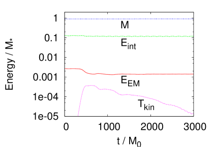
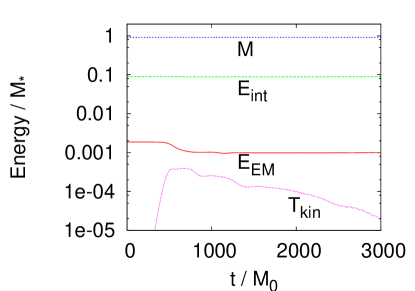
Figure 6: Evolution of the ADM mass, internal thermal, kinetic, and electromagnetic energy for model B3H (left) and model B2H (right).

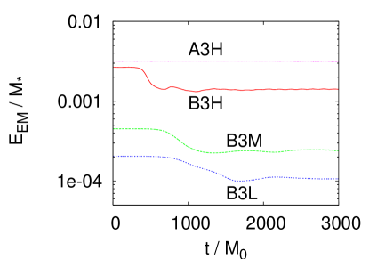
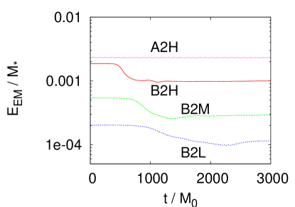
Figure 7: Left: Evolution of electromagnetic energy for models B3H, B3M, B3L, and A3H. Right: The same as the left panel but for models B2H, B2M, B2L, and A2H.

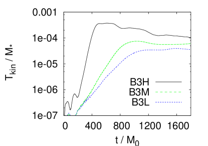
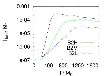
Figure 8: $T_{\rm kin}/M_{*}$ as a function of time for models B3H, B3M, and B3L (left) and for models B2H, B2M, and B2L (right).

As mentioned above, this instability always sets in for $k\geq 2$ irrespective of magnetic field strength and compactness of the neutron stars. However, the growth time scale of this instability depends strongly on the magnetic field strength. Figure 7 plots electromagnetic energy as a function of time for several models with $k=1$ (left) and $k=2$ (right). For models A3H and A2H which are stable models, it remains approximately constant, whereas for models with $k=2$, it always decreases during the evolution and the decrease time scale is shorter for the larger electromagnetic energy.

To determine the growth rate of the dynamically unstable mode, it is convenient to see $T_{\rm kin}$ because it is initially zero and increases purely due to excitation of the unstable modes. Figure 8 plots $T_{\rm kin}/M_{*}$ as a function of time for models B3H, B3M, and B3L (left) and for models B2H, B2M, and B2L (right). Note that for other unstable models, the behavior of the curve is qualitatively the same. This figure shows that after the onset of the instability, the kinetic energy increases approximately in an exponential manner with time as $\propto e^{t/\tau}$ where $\tau$ is a constant. This indicates that the instability is dynamical. This exponential growth holds for all the unstable models irrespective of the value of $k$ and magnetic field strength. Thus, we refer to $\tau$ as the growth time scale.

Table II lists approximate values of $\tau$ for all the unstable models. It is found that $\tau$ increases systematically with the decrease of magnetic field strength. In Table I, we also describe the values of $\bar{\tau}_{A}$ calculated using Eq. (21). We find that the order of magnitude of $\tau$ agrees with $\bar{\tau}_{A}$ well, and furthermore, the relation $\tau/\bar{\tau}_{A}\approx 0.3$–0.6 holds irrespective of the value of $k$ and the magnetic field strength. This indicates that the dynamical instability grows in the Alfvén time scale.

As we have reported, the instability sets in only for $k\geq 2$ and the growth time scale is approximately proportional to the Alfvén time scale. These imply that this instability is indeed the Tayler instability Tayler ; Spruit . Hereafter, we refer to this instability as the Tayler instability.

In this paper, we input a very high magnetic field strength of $\sim 10^{16}$–$10^{17}$ G. Because the scaling holds as shown above, the present result may be applied for neutron stars of canonical field strength $\sim 10^{12}$–$10^{13}$ G or magnetar field strength $\sim 10^{14}$–$10^{15}$ G. As shown in Eq. (2), the Alfvén time scale is $\sim 10$–100 ms for the magnetar field strength and $\sim 1$–10 s for the canonical field strength. Thus, the growth time scale of the Tayler instability is $\mathrel{\raise 1.29167pt\hbox{$<$}\mkern-14.0mu\lower 2.58334pt\hbox{$\sim$}}10$ s for the field strength larger than $\sim 10^{12}$ G. If this instability sets in for a neutron star, the electromagentic energy will be redistributed and transformed into kinetic energy in a short time scale (as short as or shorter than the rotation period).

Table 2: The growth time, $\tau$, of the Tayler instability for the unstable models. The third column denotes the time span of the data set which is used for deriving the growth time. The fourth column denotes ratio of $\tau$ to the averaged Alfvén time scale derived from Eq. (21). The error size of the evaluated value of $\tau$ is $\sim 3M_{0}$.

Model	$\tau/M_{0}$	$t/M_{0}$	$\tau/\bar{\tau}_{A}$
B3H	$\approx 35$	200–400	$\approx 0.48$
B3M	$\approx 95$	200–600	$\approx 0.54$
B3L	$\approx 160$	200–800	$\approx 0.61$
B2H	$\approx 40$	200-400	$\approx 0.41$
B2M	$\approx 90$	200–800	$\approx 0.49$
B2L	$\approx 170$	200–1000	$\approx 0.57$
C3L	$\approx 115$	200-700	$\approx 0.49$
C2H	$\approx 32$	150–350	$\approx 0.32$

For illustrating that the results presented so far depend only weakly on grid resolution, we show numerical results with different grid resolutions and grid structures for model B3H. The chosen grid strcuture is described in Sec. III A. Figure 9 plots the evolution of the central density, the central value of the lapse function, the electromagnetic, and kinetic energy, respectively. We also show violation of the Hamiltonian constraint and conservation of the ADM mass. Here the definition of the violation of the Hamiltonian constraint is the same as that shown in Eq. (43) of S03 ; an averaged Hamiltonian constraint is defined by using the rest-mass density as a weight. We note that the ADM mass does not have to be conserved in axial symmetry, but in the present context with negligible gravitational radiation, it should be approximately conserved.

We find that the numerical results are qualitatively the same irrespective of the grid setting, and also depend quantitatively weakly on it: At approximately the same time, the neutron star expands due to the nonlinear growth of the Tayler instability, and then, the density, the lapse function, and the electromagnetic energy relax to a stable state (besides oscillation around new equilibrium values). The minumum electromagnetic energy and the maximum kinetic energy achieved depends weakly on the grid resolution and differences among five runs are at most $\sim 20\%$. For $t\mathrel{\raise 1.29167pt\hbox{$<$}\mkern-14.0mu\lower 2.58334pt\hbox{$\sim$}}1000M_{0}$, the violation of the Hamiltonian constraint is larger for the case that non-uniform grid is employed, but this is purely due to the grid structure chosen and magnitude of the violation eventually relaxes to be small. These facts demonstrate that our choice for the grid resolution and the grid structure is appropriate for studying this type of instability. One caution is that the kinetic energy in the late time depends strongly on the grid resolution. The likely reason is that with poorer grid resolutions, numerical viscosity dissipates the circulation, resulting in the suppress of the convective energy. This is illustrated by the fact that for the case of “360H”, the kinetic energy is largest among five runs. Thus, in reality, the convective motion may be approximately constant for a time much longer than the Alfvén time scale. However, accurately following the convective motion for a long time is not main subject of this paper, and hence, we do not touch this problem in detail.

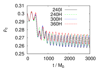
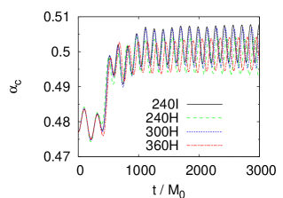
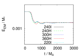
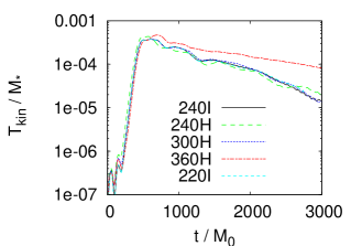
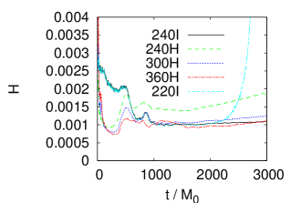
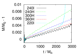
Figure 9: Evolution of central density, central value of the lapse function, electromagnetic energy, kinetic energy, violation of the Hamiltonian constraint, and violation of conservation of the ADM mass for model B3H with five different grid structures. “240I”, “220I”, “240H”, “300H”, and “360H” imply nonuniform grid with $N=240$ and $N=220$, uniform grid with $N=240$, 300, and 360, respectively. The units of time is initial ADM mass $M_{0}$. Numerical results for $\alpha_{c}$ and $\rho_{c}$ are not shown for run 220I because they are approximately the same as those for run 240I for $t\mathrel{\raise 1.29167pt\hbox{$<$}\mkern-14.0mu\lower 2.58334pt\hbox{$\sim$}}2500M_{0}$. Computation for run 220I crashes at $t\sim 2700M_{0}$.

III.2.2 Rotating case

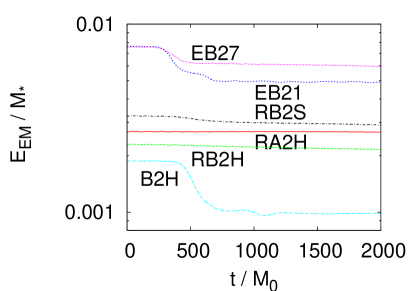
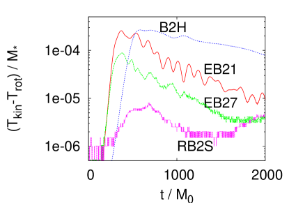
Figure 10: $E_{\rm EM}/M_{*}$ and $(T_{\rm kin}-T_{\rm rot})/M_{*}$ as functions of time for models RA2H, RB2H, RB2S, EB21, and EB27. For comparison, results for model B2H are plotted together. For models RA2H and RB2H, $(T_{\rm kin}-T_{\rm rot})/M_{*}$ remains to be smaller than $5\times 10^{-7}$.

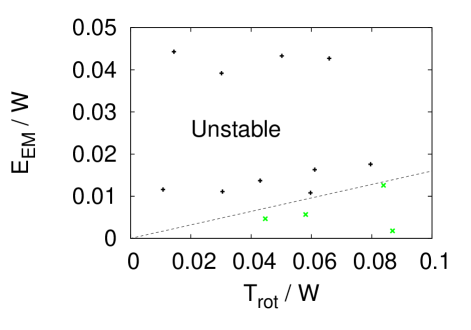
Figure 11: Results of stability properties for rotating models with $k=2$. All the stars above the dashed line are unstable, and the instability grows in the time scale of $\mathrel{\raise 1.29167pt\hbox{$<$}\mkern-14.0mu\lower 2.58334pt\hbox{$\sim$}}\bar{\tau}_{A}$. For the stars below the dashed line, instability does not grow in the Alfvén time scale, although we cannot exclude the possibility that the stars are unstable and the unstable modes grow for a time scale $\gg\bar{\tau}_{A}$.

Numerical simulations for rigidly rotating neutron stars were performed for all the models listed in Table I. We find that the stability criteria for the rotating stars are different from those for nonrotating stars. As in the nonrotating case, stars with $k=1$ are always stable against axisymmetric perturbation irrespective of magnetic field strength. Also, for many of stars with $k=2$, the Tayler instability occurs and grows approximately in the Alfvén time scale. In contrast to the nonrotating case, however, stars with $k\geq 2$ may be stable for the rapidly rotating case; at least, for the first $\sim 10$ Alfvén time scale, we do not find evidence for occurring the Tayler instability. Figure 10 plots evolution of electromagnetic and convective kinetic energy (defined by $T_{\rm kin}-T_{\rm rot}$) for models RA2H, RB2H, RB2S, EB21, and EB27. This shows that for the rapidly rotating models, RA2H and RB2H, the electromagnetic energy remains approximately constant and indicates that they are stable, at least, in the time scale of $t=2000M_{0}$, more than $10\bar{\tau}_{A}$ . It is worth noting that for model RB2H, $k=2$ and electromagnetic energy is strong as $E_{\rm EM}/W\sim 0.01$. Nevertheless, it is a stable model: This illustrates that rapid rotation suppresses the Tayler instability. By contrast, models RB2S and EB27, which have even larger electromagnetic energy $E_{\rm EM}/W\sim 0.02$–0.04, are unstable even for a large value of $T_{\rm rot}/W\sim 0.07$.

These results indicate that the stability is determined by the ratio $E_{\rm EM}/T_{\rm rot}$; i.e., the Tayler instability grows in the Alfvén time scale only when $E_{\rm EM}/T_{\rm rot}$ is larger than a critical value $\sim 0.2$. To clarify this fact, we generate Fig. 11 which summarizes the stability properties for rotating models with $k=2$. This figure indeed suggests that the Tayler instability grows only for $E_{\rm EM}/T_{\rm rot}\mathrel{\raise 1.29167pt\hbox{$>$}\mkern-14.0mu\lower 2.58334pt\hbox{$\sim$}}0.2$ (note that the dashed line denotes $E_{\rm EM}/T_{\rm rot}=0.16$). This result is in qualitative agreement with the Newtonian analysis of Appendix A.

As seen in Fig. 10, the fraction of the decrease in the electromagnetic energy during evolution is smaller for larger value of $T_{\rm rot}/W$. Also, shown is that for larger ratio of $T_{\rm rot}/E_{\rm EM}$, the maximum value of convective kinetic energy, $T_{\rm kin}-T_{\rm rot}$, is smaller and the convective motion damps more quickly for the rotating models. In particular, for the rapidly rotating case, the convective kinetic energy is smaller than the electromagnetic energy by two or three orders of magnitude. As mentioned in the previous section, the damping is partly due to the numerical dissipation. However, significant difference in the damping rates between nonrotating and rotating models suggests that the damping is primarily due to a rotational effect. All these facts indicate that rotation plays a role for stabilizing the axisymmetric unstable mode.

As discussed in Tayler2 ; Spruit , the Tayler instability induces a motion perpendicular to the rotation axis, and stabilization by rapid rotation is due to the presence of the Coriolis force. The Coriolis force pushes a fluid element, which deviates from its equilibrium location to the positive cylindrical-radial direction, to the counter-rotation direction. As a result, the centrifugal force of the fluid element is weaken, and it is enforced to return toward its equilibrium position. Thus, it is natural that the Coriolis force suppresses the onset of the Tayler instability as well as convective motion in the meridian plane.

IV Summary

In this paper, we have reported stability of neutron stars with purely toroidal magnetic fields. The stability is determined by performing GRMHD simulation. For the simulation, we prepare a variety of equilibrium neutron stars changing their compactness, strength and profile of toroidal magnetic fields, and rotational kinetic energy. The following is the summary of the numerical results.

(i) Magnetized stars with $k=1$ are stable against axisymmetric perturbation irrespective of the magnetic field strength and the rotational kinetic energy.

(ii) For the nonrotating case with $k=2$, magnetized stars are dynamically unstable irrespective of the magnetic field strength, and the magnetic field is redistributed approximately in the Alfvén time scale. The resulting profile of the magnetic fields is similar to that for $k=1$, indicating that stars with $k=1$ are attractors if only the axisymmetric perturbation is taken into account.

(iii) During the growth of the dynamically unstable modes, electromagnetic energy is transported to the kinetic energy via the Tayler instability, and as a result, a convective motion is excited. The magnitude of the convective kinetic energy becomes approximately as large as the electromagnetic energy at the time when the nonlinear growth saturates, for not-rapidly rotating neutron stars.

(iv) For the case that a neutron star is rapidly rotating, the Tayler instability is suppressed and the star with $k=2$ may be dynamically stable against axisymmetric perturbation at least in about ten Alfvén time scale. The numerical results suggest that if the rotational kinetic energy is more than $\sim 6$ times larger than the electromagnetic energy, the star is stabilized.

(v) Even for the unstable rotating models, convective motion is not induced as remarkablely as in the nonrotating case. For the rapidly rotating case in which the rotational kinetic energy is larger than the electromagnetic energy by a factor of $\mathrel{\raise 1.29167pt\hbox{$>$}\mkern-14.0mu\lower 2.58334pt\hbox{$\sim$}}2$, the maximum convective energy is smaller than the electromagnetic energy by two or three orders of magnitude. This indicates that rotation in general plays a role in stabilizing the axisymmetric Tayler instability.

As mentioned in Sec. I, protoneutron stars are likely to have strong toroidal magnetic fields if the progenitor of supernova gravitational collapse is rotating. Indeed, a number of recent MHD simulations of supernova collapse of magnetized rotating stars have shown that the toroidal magnetic field is amplified by many order of magnitude during collapse and during subsequent relaxation stage of the formed protoneutron star YS ; SKY ; TKNS ; KOTAKE ; OAM ; OADM ; ABM ; MBA ; SLSS ; DBLO ; DFD . The key mechanism in this amplification is transport of the rotational kinetic energy to the electromagnetic energy via winding induced by differential rotation. As indicated in SLSS , the electromagnetic energy could be comparable to the rotational kinetic energy at the end of the amplification. Our present numerical experiment suggests that when the condition $E_{\rm EM}/T_{\rm rot}\mathrel{\raise 1.29167pt\hbox{$>$}\mkern-14.0mu\lower 2.58334pt\hbox{$\sim$}}0.2$ is achieved, the protoneutron star may be subject to the Tayler instability.

Many of the MHD studies for supernova collapse focus on the amplification of magnetic pressure associated with the amplification of the toroidal magnetic field strength, which increases the pressure behind shock waves and can help supernova explosion or drive a strong outflow along the rotational axis. Our present study suggests that the strong toroidal magnetic field may play a role not only in increasing the pressure for pushing shock waves but also in exciting a convective motion through the Tayler instability. After the onset of this instability, a large fraction of electromagnetic energy may be transported into the convective kinetic energy. Then the convection may help to carry a hot material near the surface of a protoneutron star toward the gain region and push stalled shock waves outward Janka . As Eq. (27) indicates, the kinetic energy of the convective motion may increase to $\sim 10^{50}~{}{\rm ergs}$ if the toroidal field strength becomes $10^{16}$ G and the electromagnetic energy becomes as large as the rotational kinetic energy. This value of the kinetic energy amounts to $\sim 10\%$ of the energy required to drive supernova explosion. As we show in Fig. 5, vorticity is generated associated with the convective motion. If this vorticity is dissipated by viscosity, a large thermal energy is also generated. Such thermal energy may also contribute to pushing stalled shock waves (see similar discussion in TQB ). All these possibilities suggest that the Tayler instability should be taken into account in magnetorotational explosion scenarios for supernova explosion.

In reality, electromagnetic energy in protoneutron star at birth is likely to be much smaller than rotational kinetic energy. Thus, at its birth, the protoneutron star will be stable against the Tayler instability. Subsequently, the toroidal magnetic fields are amplified by winding caused by differential rotation, and as a result, the electromagnetic energy will reach a magnitude comparable to the rotational kinetic energy. Then, the protoneutron star could be unstable against the Tayler instability. This suggests that this instability may play a role for stopping the growth of the toroidal field strength. At the end of the toroidal field amplification, the resulting electromagnetic energy is likely to be at most comparable to the rotational kinetic energy, and hence, the instability may not be as strong as that in the nonrotating stars, as illustrated in Sec. III B. Also, the convective energy driven by the instability is likely to depend strongly on the amplification process of the toroidal magnetic fields via winding. For example, if the degree of differential rotation is largest near the rotation axis, the instability will not be strong because the configuration is likely to be similar to that of $k=1$. On the other hand, the degree of differential rotation is largest at an interior of a protoneutron star far from the rotation axis, the Taylor instability will occur. The efficiency of the winding depends strongly on the magnetic field profile and the rotational profile of progenitor. To understand the role of the Tayler instability, well-resolved, long-term MHD simulations of stellar core collapse have to be systematically performed for a number of initial conditions.

Neutron stars, observed as ordinary pulsars, typically have rotation period 0.1–1 s and magnetic field strength of $10^{11}$–$10^{13}$ G. This class of neutron stars are not subject to the Tayler instability. This is because the ratio of electromagnetic energy to rotational kinetic energy is much smaller than unity as

$${E_{\rm EM}\over T_{\rm rot}} \sim {B^{2}R^{3}/3\over I\Omega^{2}/2}$$ (28)

$$\approx 7\times 10^{-3}\biggl{(}{B\over 10^{13}~{}{\rm G}}\biggr{)}^{2}\biggl{(}{R\over 10~{}{\rm km}}\biggr{)}^{3}$$

$$~{}~{}~{}~{}~{}~{}\times\biggl{(}{I\over 10^{45}~{}{\rm g~{}cm^{2}}}\biggr{)}^{-1}\biggl{(}{\Omega\over 10~{}{\rm rad/s}}\biggr{)}^{-2},$$

where $I$ is moment of inertia.

By contrast, magnetars of rotation period 5–12 s and of magnetic field strength $10^{14}$–$10^{15}$ G WD are subject to the Tayler instability. Present numerical results imply that stable magnetars should have a magnetic field profile which is at least stable against axisymmetric perturbation.

In this paper, we focus only on the stability against axisymmetric perturbations. This work should be regarded as the first step toward deeper understanding of the Tayler instability in magnetized neutron stars. As shown in Tayler ; Acheson ; Tayler2 ; Spruit , neutron stars with toroidal magnetic fields are also unstable against nonaxisymmetric perturbation. Nonaxisymmetric Tayler instability may grow in a different manner from axisymmetric one, and hence, the dynamical evolution process of neutron stars during the growth of the unstable modes as well as the final fate could also be different. Furthermore, this instability will occur even for $k=1$. In the axisymmetric simulation, only the stars with $k\geq 2$ are unstable and magnetic field profile of such unstable star eventually relaxes to a profile similar to that with $k=1$. However, in three dimensions, such star will be still unstable. This suggests that stars may never reach a stationary state. To answer this question, GRMHD simulation in full three dimensions is required. We plan to perform three dimensional simulation in the next step.

Appendix A Perturbative analysis

In this section, we present a result of perturbative analysis on criteria for the onset of axisymmetric instabilities of neutron stars with toroidal magnetic fields. For the analysis, we follow Ref. Acheson . Newtonian gravity is assumed for the sake of clarity and simplicity, and thus, our purpose is to derive an approximate criterion for the instabilities.

Basic equations describing ideal MHD are given by

$$\partial_{t}\rho+\nabla_{i}(\rho v^{i})=0\,,$$ (29)

$$\rho\,(\partial_{t}v_{i}+v^{j}\nabla_{j}v_{i})=-\nabla_{i}\left(P+{1\over 8\pi}\,B^{j}B_{j}\right)$$

$$~{}~{}~{}~{}~{}~{}~{}~{}~{}~{}~{}~{}~{}~{}~{}~{}~{}~{}~{}~{}~{}~{}~{}~{}+{1\over 4\pi}\,B^{j}\nabla_{j}B_{i}-\rho g_{i}^{*}\,,$$ (30)

$$\partial_{t}B^{i}=\nabla_{j}(v^{i}B^{j}-v^{j}B^{i})\,,$$ (31)

$$\nabla_{i}B^{i}=0\,,$$ (32)

where $\rho$ denotes the rest-mass density, $v^{i}$ the fluid velocity, $P$ the pressure, $B^{i}$ the magnetic field, $g^{*}_{i}$ the gravitational acceleration, and $\nabla_{i}$ the covariant derivative with respect to $x^{i}$.

We derive linear perturbation equations for rigidly rotating stars with purely toroidal magnetic fields in equilibrium. The velocity and the magnetic field for the equilibrium stars are written as

$$v^{i} = (0,\Omega,0)\,,$$ (33)

$$B^{i} = \left(0,\varpi^{-1}B(\varpi,z),0\right)\,,$$ (34)

where $\Omega$ and $B(\varpi,z)$ are the angular velocity and the magnetic field strength, respectively. Here, we used the cylindrical polar coordinates $(\varpi,\varphi,z)$.

In order for the stability analysis to be tractable, we only consider axisymmetric perturbations of very short wavelength both in the $\varpi$ and $z$ directions. Here, the short wavelength implies that the wavelength, $\lambda$, of an oscillation mode is smaller than $\delta v\tau$ where $\delta v$ is a typical magnitude of the perturbed velocity field and $\tau$ is a typical change time scale of stellar structure. In other words, we perform the local analysis. We also employ the Cowling approximation, in which perturbations of the gravity are omitted.

In the short-wavelength approximation, linear perturbation equation for the mass conservation equation (29) is

$$\partial_{\varpi}\delta v^{\varpi}+\partial_{z}\delta v^{z}=0\,,$$ (35)

where $\delta Q$ denotes the Euler perturbation of the physical quantity $Q$ and we assume that $|\partial_{\varpi}\delta v^{\varpi}|\gg|\delta v^{\varpi}/\varpi|$ because of the short-wavelength approximation. Equation (35) implies that the effect of density perturbation does not play a role. This is also because of the short-wavelength approximation imposed. Thus, sound waves or $p$-modes are filtered out in this analysis.

In the short-wavelength approximation, the $\varpi$ and $z$ components of Eq. (30) become the following same equation

$$\delta P+{1\over 4\pi}\,\varpi B\,\delta B^{\varphi}=0\,.$$ (36)

The other pieces of independent information extracted from Eq. (30) are given by

$$\partial_{t}\delta v_{\varphi}+2\varpi\Omega\,\delta v^{\varpi}={1\over 4\pi}\,\delta B^{j}\partial_{j}(\varpi B)\,,$$ (37)

$$\rho[\partial_{t}(\partial_{z}\delta v_{\varpi}-\partial_{\varpi}\delta v_{z})-2\varpi\Omega\,\partial_{z}\delta v^{\varphi}]$$

$$~{}~{}~{}~{}~{}={1\over 4\pi}\,(-2B\,\partial_{z}\delta B^{\varphi})-g_{\varpi}\partial_{z}\delta\rho+g_{z}\partial_{\varpi}\delta\rho\,,~{}~{}~{}$$ (38)

where $g_{i}$ is the apparent gravity, defined by

$$g_{i}\equiv g_{i}^{*}+u^{j}\nabla_{j}u_{i}=(g^{*}_{\varpi}-\varpi\Omega^{2},0,g^{*}_{z})\,.$$ (39)

The induction equation (31) gives

$$\partial_{t}\delta B^{\varpi}=0\,,\quad\partial_{t}\delta B^{z}=0\,,$$ (40)

$$\partial_{t}\delta B^{\varphi}={B\over\varpi\rho}\,\partial_{t}\delta\rho-\rho\,\delta v^{j}\partial_{j}\left({B\over\varpi\rho}\right)\,.$$ (41)

In this study, we focus on adiabatic oscillations. Then, the relationship between $\delta P$ and $\delta\rho$ is

$$\delta P+\xi^{i}\partial_{i}P={P\Gamma\over\rho}\,(\delta\rho+\xi^{i}\partial_{i}\rho)\,,$$ (42)

where $\Gamma$ denotes the adiabatic index, defined by

$$\Gamma\equiv\left({\ln P\over\ln\rho}\right)_{\rm ad}\,,$$ (43)

and $\xi^{i}$ the Lagrangian displacement, which obeys

$$\delta v^{i}=\partial_{t}\xi^{i}+v^{j}\partial_{j}\xi^{i}-\xi^{j}\partial_{j}v^{i}\,.$$ (44)

For the axisymmetric perturbation with $v^{j}=\Omega\delta_{\varphi}^{~{}j}$, Eq. (44) reduces to

$$\delta v^{i}=\partial_{t}\xi^{i}\,.$$ (45)

Then, Eq. (42) becomes

$${1\over v_{s}^{2}\rho}\,\partial_{t}\delta P={1\over\rho}\,\partial_{t}\delta\rho+\delta v^{i}A_{i}\,,$$ (46)

where $v_{s}$ is the adiabatic sound speed, defined by

$$v_{s}\equiv\left({P\Gamma\over\rho}\right)^{1\over 2}\,,$$ (47)

and $A_{i}$ the Schwarzschild discriminant,

$$A_{i}\equiv\partial_{i}\ln\rho-{1\over\Gamma}\,\partial_{i}\ln P\,.$$ (48)

As shown in Eq. (40), we have $\delta B^{\varpi}=0=\delta B^{z}$ because we are not interested in time-independent perturbations. Thus, Eqs. (35)–(38), (41), and (46) are six independent equations for the six independent variables $\delta v^{i}$, $\delta B^{\varphi}$, $\delta\rho$, and $\delta P$. In the local analysis, axisymmetric perturbations can be written as

$$\delta Q(t,\varpi,z)=Q_{0}\exp\{i(-\sigma t+l\varpi+nz)\}\,,$$ (49)

where $Q_{0}$ is a constant, $\sigma$ the oscillation frequency, and $(l,n)$ the meridional wavenumber vector.

Substituting Eq. (49) into the perturbation equations, we obtain the following dispersion relation for $\sigma$:

$$\left(1+{v_{A}^{2}\over v_{s}^{2}}\right){s^{2}\over n^{2}}\,\sigma^{2}=4\Omega^{2}\left(1+{v_{A}^{2}\over v_{s}^{2}}\right)-\left(\hat{g}+{2v_{A}^{2}\over\varpi}\right)A_{h}$$

$$~{}~{}~{}~{}~{}~{}~{}~{}~{}~{}~{}~{}~{}~{}~{}~{}~{}~{}~{}~{}~{}+\left(\hat{g}-{2v_{s}^{2}\over\varpi}\right){v_{A}^{2}\over v_{s}^{2}}{\partial\over\partial q}\ln\left({B\over\varpi\rho}\right)\,.$$ (50)

Here, $v_{A}$ denotes the Alfvén speed

$$v_{A}\equiv\left({B^{2}\over 4\pi\rho}\right)^{1\over 2}\,,$$ (51)

$s$ the total meridional wavenumber

$$s\equiv(l^{2}+n^{2})^{1\over 2}\,,$$ (52)

$\hat{g}$ the apparent gravity along the constant phase or crests

$$\hat{g}\equiv g_{\varpi}-{l\over n}\,g_{z}\,,$$ (53)

$A_{h}$ the Schwarzschild discriminant along the constant phase or crests

$$A_{h}\equiv A_{\varpi}-{l\over n}\,A_{z}\,,$$ (54)

and $\partial/\partial q$ the derivative along the constant phase or crests

$${\partial\over\partial q}\equiv{\partial\over\partial\varpi}-{l\over n}\,{\partial\over\partial z}\,.$$ (55)

The first, the second, and the third terms in the right-hand side of Eq. (50) are related to effects of the rigid rotation, the stratification (the buoyancy), and the magnetic buoyancy, respectively. Here, it should be emphasized that the effect of rigid rotation operates as a stabilizing agent because the first term in the right-hand side of Eq. (50) is always positive.

The stabilities are determined by the dispersion relation (50). Specifically, the sign of its right-hand side determines the local stabilities; the stars are locally stable (unstable) if $\sigma^{2}>0$ ($\sigma^{2}<0$). From Eqs. (53)–(55), we find that the right-hand side of Eq. (50) is a quadratic in $l/n$, given by

$$\left(1+{v_{A}^{2}\over v_{s}^{2}}\right){s^{2}\over n^{2}}\,\sigma^{2}=a\left({l\over n}\right)^{2}+b\left({l\over n}\right)+c\,,$$ (56)

where

$$a \equiv g_{z}\left\{-A_{z}+{v_{A}^{2}\over v_{s}^{2}}{\partial\over\partial z}\ln\left({B\over\varpi\rho}\right)\right\}\,,$$ (57)

$$b \equiv \left(g_{\varpi}+{2v_{A}^{2}\over\varpi}\right)A_{z}+g_{z}A_{\varpi}$$ (58)

$$~{}~{}~{}~{}~{}~{}~{}-\left(g_{\varpi}-{2v_{s}^{2}\over\varpi}\right){v_{A}^{2}\over v_{s}^{2}}{\partial\over\partial z}\ln\left({B\over\varpi\rho}\right)$$

$$~{}~{}~{}~{}~{}~{}~{}-g_{z}{v_{A}^{2}\over v_{s}^{2}}{\partial\over\partial\varpi}\ln\left({B\over\varpi\rho}\right)\,,$$

$$c \equiv 4\Omega^{2}\left(1+{v_{A}^{2}\over v_{s}^{2}}\right)-\left(g_{\varpi}+{2v_{A}^{2}\over\varpi}\right)A_{\varpi}$$ (59)

$$~{}~{}~{}~{}~{}~{}~{}~{}+\left(g_{\varpi}-{2v_{s}^{2}\over\varpi}\right){v_{A}^{2}\over v_{s}^{2}}{\partial\over\partial\varpi}\ln\left({B\over\varpi\rho}\right)\,.$$

We therefore see that the stability condition $\sigma^{2}>0$ for any value of $l/n$ is equivalent to the condition that the three inequalities $a>0$, $c>0$, and $b^{2}-4ac<0$ are simultaneously satisfied. Contrapositively, it is found that the star is unstable if any of the following three conditions is satisfied:

$$4\Omega^{2}\left(1+{v_{A}^{2}\over v_{s}^{2}}\right)-\left(g_{\varpi}+{2v_{A}^{2}\over\varpi}\right)A_{\varpi}$$

$$~{}~{}~{}~{}~{}~{}~{}+\left(g_{\varpi}-{2v_{s}^{2}\over\varpi}\right){v_{A}^{2}\over v_{s}^{2}}{\partial\over\partial\varpi}\ln\left({B\over\varpi\rho}\right)<0\,,$$ (60)

$$g_{z}\left\{-A_{z}+{v_{A}^{2}\over v_{s}^{2}}{\partial\over\partial z}\ln\left({B\over\varpi\rho}\right)\right\}<0\,,$$ (61)

$$g_{z}\biggl{[}{v_{A}^{2}}\left\{A_{z}{\partial\over\partial\varpi}\ln\left({B\over\varpi\rho}\right)-A_{\varpi}{\partial\over\partial z}\ln\left({B\over\varpi\rho}\right)\right\}$$

$$~{}~{}~{}~{}~{}+{2\varpi\Omega^{2}}\left\{{v_{A}^{2}\over v_{s}^{2}}{\partial\over\partial z}\ln\left({B\over\varpi\rho}\right)-A_{z}\right\}\biggr{]}<0\,.$$ (62)

Here, the final equation (62) is equivalent to the condition $b^{2}-4ac>0$.

Neutron stars are likely to be stably stratified because of their strong composition gradient Reisenegger:1992 . As a result, the buoyancy inside the neutron star exerts as a stabilizing force as shown in Eqs. (60) and (61). Equation (60) also shows that the criterion of the magnetic instability depends on whether the region considered is located inside or outside the critical surface whose cylindrical radius is defined by

$$\varpi_{c}\equiv{2v_{s}^{2}\over g_{\varpi}}\,.$$ (63)

Inside (Outside) the critical surface, if ${\partial\over\partial\varpi}\ln\left({B/\varpi\rho}\right)>0$ (${\partial\over\partial\varpi}\ln\left({B/\varpi\rho}\right)<0$), the third term of Eq. (60) becomes negative and the instability is promoted.

Finally, we examine the magnetic stability of a particular model, a slowly rotating star containing toroidal magnetic fields. We assume that matter distribution of the star is spherical (namely the magnetic and centrifugal forces are not strong enough to modify this spherical shape). As an example, an $n=1$ polytropic sphere is considered because the analytic solution is available. Its matter distribution is given by

$$\rho = \rho_{0}\left({\sin(r/r_{0})\over(r/r_{0})}\right)\,,$$ (64)

$$P = P_{0}\left({\sin(r/r_{0})\over(r/r_{0})}\right)^{2}\,,$$ (65)

where $\rho_{0}$ and $P_{0}$ are the central values of the density and the pressure, respectively, and $r_{0}$ is stellar radius

$$r_{0}\equiv\left({2P_{0}\over 4\pi G\rho_{0}^{2}}\right)^{1\over 2}\,.$$

For the magnetic field distribution, we take a simple form, as in KY , as

$$B=b_{0}(\rho/\rho_{0})^{k}(r\sin\theta/r_{0})^{2k-1}\,,$$ (66)

where $b_{0}$ and $k$ are constants. Regularity of the magnetic fields around the magnetic axis requires that $k$ is a positive integer. Here, we used the polar coordinates $(r,\theta,\varphi)$. Note that this magnetic field distribution is the Newtonian limit of that used in the present GRMHD simulation. In this analysis, we omit the buoyancy or take $A_{i}=0$ to focus on the magnetic instability.

First, we pay attention to the nonrotating case. Then, the instability conditions (60) and (61) are written as

$$D_{1}(r,\theta) \equiv {r_{0}^{2}\over v_{A,0}^{2}}\left(g_{\varpi}-{2v_{s}^{2}\over r\sin\theta}\right){v_{A}^{2}\over v_{s}^{2}}\left(\sin\theta{\partial\over\partial r}+{\cos\theta\over r}{\partial\over\partial\theta}\right)$$ (67)

$$~{}~{}~{}~{}~{}~{}~{}\times\ln\left({B\over\rho\,r\sin\theta}\right)<0\,,$$

$$D_{2}(r,\theta) \equiv {r_{0}^{2}\over v_{A,0}^{2}}g_{z}{v_{A}^{2}\over v_{s}^{2}}\,\left(\cos\theta{\partial\over\partial r}-{\sin\theta\over r}{\partial\over\partial\theta}\right)$$ (68)

$$~{}~{}~{}~{}~{}~{}~{}\times\ln\left({B\over\rho\,r\sin\theta}\right)<0\,,$$

Note that by definition, $D_{1}$ and $D_{2}$ are dimensionless quantities and are independent of the magnetic field strength $b_{0}$. The left-hand side of Eq. (62) vanishes in the present situation and this third instability condition cannot give any useful information. For the case of $k=1$, it can be seen that $D_{1}=0=D_{2}$ because $\partial_{i}\ln(B/\rho\,r\sin\theta)\propto k-1$. Thus, the star is neutrally stable for $k=1$. In Fig. 12, we give the distributions of $D_{1}$ and $D_{2}$ on the meridional cross section for the case of $k=2$. In this figure, the darker regions have locally larger growth rates of the unstable mode, whereas the white regions correspond to neutrally stable ones (regions of $D_{1}\approx 0$ and $D_{2}\approx 0$). We then see that the magnetized stars with $k=2$ are indeed locally unstable. In Fig. 12, we confirm that the unstable regions determined by the criterion $D_{1}$ are separated by the the critical surface.

The instability determined by $D_{1}$ occurs primarily near the equatorial plane and relatively high-density region. By contrast, the instability determined by $D_{2}$ occurs near the surface and for the region of relatively weak magnetic field, and this indicates that this mode plays a minor role for redistribution of the magnetic field and for inducing convection. The instability found in our numerical simulation is likely to be associated with the mode determined by $D_{1}$. Hence, in the following, we focus primarily on this mode.

The modes associated with $D_{1}$ and $D_{2}$ determine the instability in particular for $l/n\rightarrow 0$ and $l/n\rightarrow\infty$, respectively. Thus, we focus on the case for small values of $l/n$. As discussed in Spruit ; Tayler2 , the Tayler instability is associated with a motion perpendicular to the magnetic axis. This type of motion corresponds to the limit of $l/n\rightarrow 0$ in this analysis because $\delta v^{z}=-(l/n)\delta v^{\varpi}$ (see Eq. (35)). Thus, from this point of view, it is reasonable to pay attention for the mode associated with $D_{1}$.

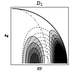
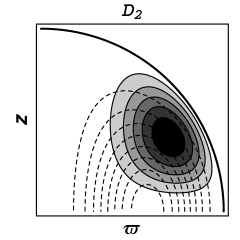
Figure 12: Contours curves (solid curves) of $D_{1}$ (left) and $D_{2}$ (right) on the meridional cross section for the $n=1$ polytropic star containing weak toroidal magnetic fields with $k=2$. The darker regions are locally more unstable, whereas the white regions correspond to neutrally stable ones (regions with $D_{1}\approx 0\approx D_{2}$). The contours of equi-$D$ are linearly spaced; the difference between two adjacent contours is a sixth of the difference between the maximum and minimum values of $D_{1}$ and $D_{2}$. The maximum value is zero and the minimum values are $-4.96$ and $-1.07$ for $D_{1}$ and $D_{2}$, respectively. The thick quarter circle denotes the surface of the star. Inside the star, the dashed curves and the dashed-dotted curve show equi-$B$ contours and the critical surface, respectively.

Because the Tayler instability occurs for the magnetic field with $k=2$ as discussed above, henceforth, we only consider the case of $k=2$. For this model, the averaged Alfvén speed $\bar{v}_{A}$ is given by

$$\bar{v}_{A} = \left({\displaystyle\int B^{2}d^{3}x\over\displaystyle 4\pi\int\rho\,d^{3}x}\right)^{1\over 2}\,$$ (69)

$$= \left\{{3\over 2800}(315-200\pi^{2}+32\pi^{4})\right\}^{1\over 2}v_{A,0}\,$$

$$\approx 1.25\,v_{A,0}\,.$$

where $v_{A,0}$ is defined as

$$v_{A,0}\equiv{b_{0}\over\sqrt{4\pi\rho_{0}}}\,.$$

The growth time $\tau$ for the Tayler instability defined in Sec. III is associated with increase in the kinetic energy. The growth time $\tau$ for the most unstable mode is therefore given by

$$\tau/\bar{\tau}_{A}=(2\sigma\bar{\tau}_{A})^{-1}\approx 0.199\,{\rm Min}\left({v_{A,0}\over r_{0}\,\sigma}\right)\,,$$ (70)

where ${\rm Min}(Q)$ denotes the minimum value of $Q(r,\theta)$. In the weak magnetic field approximation assumed, $v_{A,0}(r_{0}\,\sigma)^{-1}$ is given by

$${v_{A,0}\over r_{0}\,\sigma}=\left\{{1+\left({l\over n}\right)^{2}\over\left|D_{2}\left({l\over n}\right)^{2}+\tilde{b}\left({l\over n}\right)+D_{1}\right|}\right\}^{1\over 2}\,,$$ (71)

where $\tilde{b}=(r_{0}^{2}v_{A,0}^{-2})\,b$. In Fig. 13, we show the growth time $\tau/\bar{\tau}_{A}$ obtained by the local analysis as a function of $l/n$. As mentioned above, we focus on the case that $l/n$ is small. Then, Fig. 13 shows that the unstable mode characterized by $l/n=0$ is the most unstable one, whose growth time is given by

$$\tau/\bar{\tau}_{A}\approx 0.089\,.$$ (72)

Thus, the minimum growth time is by a factor of 3–5 shorter than that obtained by the GRMHD simulations (compare with Table II), but the order of magnitude agrees. For modes with a moderate value of $l/n$, as shown in Fig. 13, the growth time $\tau/\bar{\tau}_{A}$ increases. For a mode with $l/n\approx 2$, for example, $\tau/\bar{\tau}_{A}\approx 0.2$, which is 1/3–2/3 of the growth time shown in Table II. This result is reasonable because we here assume a Newtonian model whereas in the simulations, we adopt highly general relativistic neutron stars for which the profiles of density and magnetic field are significantly different from the Newtonian ones.

Figure 13: Growth time $\tau/\bar{\tau}_{A}$ for the most unstable mode, given as a function of $l/n$.

Figure 14: Critical ratio of the electromagnetic energy to the rotational kinetic energy, $\left(E_{\rm EM}/T_{\rm rot}\right)_{c}$, given as a function of $l/n$.

Next, we consider the slowly rotating model. In the slow rotation and weak magnetic field approximation, the criterion of the Tayler instability becomes

$${r_{0}^{2}\Omega^{2}\over v_{A,0}^{2}}+{1\over 4}\left\{D_{2}\left({l\over n}\right)^{2}+\tilde{b}\left({l\over n}\right)+D_{1}\right\}<0\,.$$ (73)

For the $k=2$ model, the rotational kinetic energy $T_{\rm rot}$ and the electromagnetic energy $E_{\rm EM}$ are, respectively, given by

$$T_{\rm rot} = {1\over 2}\int\rho\,r^{2}\sin^{2}\theta\Omega^{2}\,d^{3}x\,$$ (74)

$$= {4\over 3}\pi^{2}(\pi^{2}-6)\rho_{0}r_{0}^{5}\Omega^{2}\,$$

$$\approx 50.9\,\rho_{0}r_{0}^{5}\Omega^{2}\,,$$

$$E_{\rm EM} = {1\over 8\pi}\int B^{2}\,d^{3}x\,$$ (75)

$$= {3\pi\over 5600}(315-200\pi^{2}+32\pi^{4})r_{0}^{3}b_{0}^{2}\,$$

$$\approx 2.45\,r_{0}^{3}b_{0}^{2}\,.$$

The ratio of the electromagnetic energy to the rotational kinetic energy is then written as

$$E_{\rm EM}/T_{\rm rot}\approx 0.605\,{v_{A,0}^{2}\over r_{0}^{2}\Omega^{2}}\,.$$ (76)

In terms of $E_{\rm EM}/T_{\rm rot}$, thus, Eq. (73) is rewritten as

$$E_{\rm EM}/T_{\rm rot} > \left(E_{\rm EM}/T_{\rm rot}\right)_{c}\,$$ (77)

$$\equiv {\rm Min}\left({-2.42\over D_{2}\left({l\over n}\right)^{2}+\tilde{b}\left({l\over n}\right)+D_{1}}\right)\,.$$

For the polytropic models with $n=1$ and $k=2$, numerical values of $\left(E_{\rm EM}/T_{\rm rot}\right)_{c}$ are shown as a function of $l/n$ in Fig. 14.

Form this figure, it is found that for the most unstable mode, whose value of $l/n$ is zero, the Tayler instability sets in if the condition,

$$E_{\rm EM}/T_{\rm rot}>0.49\,,$$ (78)

is satisfied. For modes with a moderate value of $l/n$, values of $\left(E_{\rm EM}/T_{\rm rot}\right)_{c}$ decreases, e.g. $\left(E_{\rm EM}/T_{\rm rot}\right)_{c}\approx 0.21$ for a mode with $l/n\approx 2$. As argued in Sec. III, the instability condition obtained by the GRMHD simulation is $E_{\rm EM}/T_{\rm rot}\mathrel{\raise 1.29167pt\hbox{$>$}\mkern-14.0mu\lower 2.58334pt\hbox{$\sim$}}0.2$, which is the same order as that of Eq. (78).

For the small values of $E_{\rm EM}/T_{\rm rot}$, the unstable modes should have larger values of $l/n$, and correspondingly, the growth time scale becomes longer. This suggests that even if a model star appears to be stable in a numerical simulation for a finite duration, the star might become unstable for a sufficiently long run.

As found from Fig. 14, magnetized star is always unstable for modes with $|l/n|\approx\infty$ irrespective of the rotation rate. As mentioned previously, however, these modes are associated with $D_{2}$. This instability occurs near the stellar surface and its effect would not be significant for global redistribution of the magnetic field profile. Thus, although all the magnetized stars with $k=2$ are unstable strictly speaking, this type of instability does not seem to play a significant role.

References

- (1) A. Lyne and F. Graham-Smith, Pulsar Astronomy (Cambridge University Press, 2005).
- (2) P. M. Woods and C. Thompson, in Compact Stellar X-ray Sources, edited by W. H. G. Lewin and M. van der Klis (Cambridge University Press, 2006)
- (3) S. Akiyama, J. C. Wheeler, D. L. Meier, and I. Lichtenstadt, Astrophys. J. 584, 954 (2003).
- (4) M. Shibata, Y.-T. Liu, S. L. Shapiro, and B. C. Stephens, Phys. Rev. D 74, 104026 (2006).
- (5) H. C. Spruit, astro-ph/0711.3650.
- (6) R. J. Tayler, Mon. Not. R. Astro. Soc. 161, 365 (1973).
- (7) J. D. Acheson, Phil. Trans. Roy. Soc. Lond. A 289, 459 (1978)
- (8) E. Pitts and R. J. Tayler, Mon. Not. R. Astro. Soc. 216, 139 (1985).
- (9) H. C. Spruit, Astron. and Astrophys., 349, 189 (1999).
- (10) M. Shibata and Y.I. Sekiguchi, Phys. Rev. D 72, 044014 (2005).
- (11) K. Kiuchi and S. Yoshida, submitted to PRD (arXiv:0802.2983[astro-ph]).
- (12) M. Shibata and T. Nakamura, Phys. Rev. D 52, 5428 (1995); T. W. Baumgarte and S. L. Shapiro, Phys. Rev. D 59, 024007 (1998).
- (13) M. Alcubierre, S. Brandt, B. Brügmann, D. Holz, E. Seidel, R. Takahashi, and J. Thornburg, Int. J. Mod. Phys. D 10, 273 (2001); M. Shibata, Prog. Theor. Phys. 104, 325 (2000).
- (14) M. Shibata, Phys. Rev. D 67, 024033 (2003).
- (15) M. Shibata, Astrophys. J. 595, 992 (2003); M. Shibata and Y.I. Sekiguchi, Phys. Rev. D 69, 084024 (2004).
- (16) A. Kurganov and E. Tadmor, J. Comput. Phys. 160, 214 (2000).
- (17) A. Lucas-Serrano, J. A. Font, J. M. Ibánez, and J. M. Martí, Astron. Astrophys. 428, 703 (2004).
- (18) M. D. Duez, Y. T. Liu, S. L. Shapiro, M. Shibata, and B. C. Stephens, Phys. Rev. Lett. 96, 031101 (2006); M. Shibata, M. D. Duez, Y. T. Liu, S. L. Shapiro, and B. C. Stephens, Phys. Rev. Lett. 96, 031102 (2006).
- (19) M. D. Duez, Y. T. Liu, S. L. Shapiro, M. Shibata, and B. C. Stephens, Phys. Rev. D, 73, 104015 (2006).
- (20) G. B. Cook, S. L. Shapiro, and S. A. Teukolsky, Astrophys. J. 422, 227 (1994).
- (21) S. Yamada and H. Sawai, Astrophys. J. 608, 907 (2004).
- (22) H. Sawai, K. Kotake, and S. Yamada, Astrophys. J. 631, 446 (2005).
- (23) T. Takiwaki, K. Kotake, S. Nagataki, and K. Sato, Astrophys. J. 616, 1086 (2004).
- (24) K. Kotake, H. Sawai, S. Yamada, and K. Sato, Astrophys. J. 608, 391 (2004).
- (25) M. Obergaulinger, M. A. Aloy, and E. Müller, Astron. Astrophys., 450, 1107 (2006).
- (26) M. Obergaulinger, M. A. Aloy, H. Dimmelmeier, and E. Müller, submitted to Astron. Astrophys. (astro-ph/0602187).
- (27) N. V. Adreljan, G. S. Bisnobatyi-Kogan, and S. G. Moiseenko, Mon. Not. R. Astro. Soc. 359, 333 (2005).
- (28) S. G. Moiseenko, G. S. Bisnobatyi-Kogan, and N. V. Adreljan, Mon. Not. R. Astro. Soc. 370, 501 (2006).
- (29) L. Dessart, A. Burrow, E. Livne, and C. D. Ott, Astrophys. J. 669 585 (2007); 673, L43 (2008).
- (30) P. Cerdá-Durán, J. A. Font, and H. Dimmelmeier, Astron. Astrophys. 474, 169 (2007); P. Cerdá-Durán, J. A. Font, L. Ant’on, and E. Müller, astro-ph/0804.4572.
- (31) H.-T. Janka, Astron. Astrophys. 368, 527 (2001).
- (32) T. A. Thompson, E. Quataert, and A. Burrows, Astrophys. J. 620, 861 (2005).
- (33) A. Reisenegger and P. Goldreich, Astrophys. J. 395, 240 (1992).