Bayesian approach to clustering real value, hypergraph and bipartite graph data:
solution via variational methods

Abstract

Data clustering, including problems such as finding network communities, can be put into a systematic framework by means of a Bayesian approach. The application of Bayesian approaches to real problems can be, however, quite challenging. In most cases the solution is explored via Monte Carlo sampling or variational methods. Here we work further on the application of variational methods to clustering problems. We introduce generative models based on a hidden group structure and prior distributions. We extend previous attends by Jaynes, and derive the prior distributions based on symmetry arguments. As a case study we address the problems of two-sides clustering real value data and clustering data represented by a hypergraph or bipartite graph. From the variational calculations, and depending on the starting statistical model for the data, we derive a variational Bayes algorithm, a generalized version of the expectation maximization algorithm with a built in penalization for model complexity or bias. We demonstrate the good performance of the variational Bayes algorithm using test examples.

I Introduction

Mixture models provide an intuitive statistical representation of datasets structured in groups, clusters or classes McLachlan and Peel (2000). A complex dataset is decomposed into the superposition of simpler datasets. The inverse problem consists in determining the group decomposition and the statistical parameters characterizing each group. For a fixed number of groups the expectation maximization (EM) algorithm provides a recursive solution to the inverse problem Dempster et al. (1977). The estimation of the right number or groups has been, however, a great challenge. Corrections such as the Arkaike information criterion (AIC) Akaike (1974) and the Bayesian information criterion (BIC) Schwarz (1978) have been derived, penalizing model complexity and overfitting. Yet, the number of groups estimated from these criteria is in general unsatisfactory.

In contrast, a Bayesian approach would not attempt to estimate what is the “optimal” number of groups, but instead average over models with a different number of groups Jeffreys (1939). The Bayesian approach is becoming a popular technique to solve problems in data analysis, model selection and hypothesis testing Spirtes et al. (2000); MacKay (2003); Robert (2007). Many of the original ideas come from the early work of Jeffreys Jeffreys (1939), but it is just recently that they are starting to be used widely Spirtes et al. (2000); MacKay (2003); Robert (2007). The application of Bayesian approaches to real problems can be, however, quite challenging. In most cases the solution is explored via Monte Carlo sampling Chen et al. (2000); MacKay (2003) or variational methods MacKay (2003); Beal ; Yedidia et al. (2005). The application of variational methods to Bayesian problems results in the variational Bayes (VB) algorithm MacKay (2003); Beal . The VB algorithm is a set of self-consistent equations analog to the EM algorithm. They can be solved recursively obtaining an approximate solution to the inverse inference problem. These methods have been applied, for example, to Gaussian mixture models for real value data McLachlan and Peel (2000); Rasmussen (2000), Dirichlet mixture models for categorical data Blei et al. (2003) and the problem of finding graph modules Hofman and Wiggins .

Here we further study the use of variational methods in the context of Bayesian approaches, focusing on data clustering problems. I the first two sections we review the Bayesian approach. In Section II we revisit the connection between the Bayesian formulation and statistical mechanics. In section III we introduce the generalities of generative models with a hidden structure at the samples side and at both the samples and variables side. In Section IV we extend the previous work by Jaynes Jaynes (1969) deriving prior distributions based on symmetry properties. We report a correction to his result for the model with a location and scale parameter and an extension of his result for the binomial model to the multinomial model. In the following Sections we study the problem of two-sides clustering real value data and of clustering data represented by a hypergraph or bipartite graph. Depending on our starting statistical model, we obtain a VB algorithm. Because of its Bayesian root, the VB algorithms have a built in correction for model complexity or bias and, therefore, they do not require the use of additional complexity criteria. The performance of the VB algorithms is tested in some examples, obtaining satisfactory results whenever there is a significant distinction between the groups.

II Bayesian approach and variational solution

The Bayesian approach is a systematic methodology to interpret complex datasets and to evaluate model hypothesis. Its main ingredients or steps are: given a dataset $D$, (i) introduce a statistical model with model parameters, $\phi$, (ii) write down the likelihood to observe the data given the proposed model and parameters, $P(D|\phi)$, (iii) determine the prior distribution for the model parameters based on our current knowledge, $P(\phi)$, and, finally, (iv) invert the statistical model of the data given the likelihood and prior distribution to obtain the posterior distribution of the model parameters given the model and data, $P(\phi|D)$. The latter step is based on Bayes rule

$$P(\phi|D)=\frac{1}{Z}P(D|\phi)P(\phi)$$ (1)

where

$$Z=P(D)=\int d\theta P(D|\phi)P(\phi)\ .$$ (2)

Having obtained the distribution of the model parameters, at least formally, we can determine other magnitudes. For example, the average of a quantity $A(\phi)$ is given by

$$\langle A(\phi)\rangle=\int d\phi P(\phi|D)A(\phi)\ .$$ (3)

In practice calculating (2) or (3) is a formidable task. A very powerful approximation scheme is the variational method MacKay (2003); Beal . The main idea of the variational method is to approximate the generally difficult to handle distribution $P(\phi|D)$ by a distribution $Q(\phi|D)$ of a more tractable form. In the following we omit the dependency of $Q$ on $D$ and just write $Q(\phi)$. Given $Q(\phi)$ we can obtain a bound for $F=-\ln Z$ using Jensen’s inequality

$$F = -\ln Z$$ (4)

$$= -\ln\int d\phi Q(\phi)\frac{P(D|\phi)P(\phi)}{Q(\phi)}$$

$$\leq -\int d\phi Q(\phi)\ln\frac{P(D|\phi)P(\phi)}{Q(\phi)}$$

The latter equation can be rewritten as MacKay (2003)

$$F\leq U-TS$$ (5)

where $T=1$,

$$U=-\int d\phi Q(\phi)\ln P(D|\phi)$$ (6)

is minus the average log likelihood and

$$S=-\int d\phi Q(\phi)\ln\frac{Q(\phi)}{P(\phi)}$$ (7)

is the Kullback-Leibler divergence of $Q(\phi)$ relative to the prior distribution $P(\phi)$ Kullback (1959). Equation (5) resembles the usual free energy in statistical mechanics: $F=U-TS$, where $U$, $S$ and $T$ are the internal energy, entropy and temperature of the system, the temperature being expressed in units of the Boltzman constant $k_{\rm B}$. Minus the average log likelihood plays the role of the internal energy, the Kullback-Leibler divergence of $Q(\phi)$ plays the role of the entropy and temperature equals one.

Equation (5) emphasizes the two components determining the best choice of variational distribution $Q(\phi)$: better fit to the data and model bias. How well the data is fitted is quantified by the internal energy $U$ (6). To achieve the best fit, or internal energy ground state, $Q(\phi)$ should be concentrated around the regions of the parameter space where $P(D|\phi)$ is maximum. The best choice in this respect will by the maximum likelihood estimate (MLE)

$$Q_{\rm MLE}(\phi)=\delta(\phi-\phi^{*})$$ (8)

where

$$\phi^{*}=\max_{\phi}P(D|\phi)\ .$$ (9)

In the opposite extreme, when no data is presented to us, the best distribution is that maximizing the Kullback-Leibler divergence relative to the prior distribution. This maximum entropy (ME) solution is the prior distribution itself

$$Q_{ME}(\phi)=P(\phi)\ .$$ (10)

In general, the drive to better fit the data is opposed by the tendency to obtain the least unbiased model. The variational solution is therefore in the middle between the one extreme of biased models fitting the data very well and completely unbiased models giving a bad fit to the data. It is obtained after minimizing (5) with respect to $Q(\phi)$ over a restricted class of functions. This variational solution $Q(\phi)$ represents the closest distribution to $P(\phi|D)$ within the class of functions considered.

III Statistical model with a population structure

In this section we present the generalities of statistical models with a first level population structure. Similar models has been studied in Blei et al. (2003); Hofman and Wiggins . Our working hypothesis is that there is a hidden population structure, characterized by the subdivision of the population samples into groups. We assume that we are given a dataset $D$ which, in some way to be determined, reflects the population structure. The problem consist in inferring this hidden structure and the associated model parameters from the data. To tackle this problem we introduce a statistical model with a built in population structure as a generative model of the data. The population structure and the model parameters are then inferred solving the inverse problem. More precisely

• We consider a population composed of $n$ elements divided in $K$ groups.

• The samples assignment to groups is generated by a multinomial model with probabilities $\pi_{k}$, $k=1,\ldots,K$. Denoting by $g_{i}$ the group to which the $i$-th sample belongs, we obtain

  $$P(g|\pi)=\prod_{i=1}^{n}\pi_{g_{i}}\ .$$ (11)

• Given the group assignments $g_{i}$, and depending on the dataset, we write down the likelihood $P(D|g,\theta)$ to observe the data parametrized by the parameter set $\theta$.

• Putting all this together we obtain the posterior distribution

  $$P(\phi|D)=\frac{1}{Z}P(D|g,\theta)P(g|\pi)P(\theta)P(\pi)P(K)\ ,$$ (12)

  where $\phi=(g,\theta,\pi,K)$ and $P(\theta)$, $P(\pi)$ and $P(K)$ are the prior distributions of $\theta$, $\pi$ and $K$.

The form of the prior distributions, except for $P(K)$, is the subject of the next section. The distribution $P(K)$ is irrelevant for problems with large datasets. The difference between the log-likelihood of models with different values of $K$ is in general of the order of the dataset size and, as a consequence, the contribution of $\ln P(K)$ is negligible. Thus, in the following sections we simply neglect the contribution given by $P(K)$. Finally, we specify the likelihood $P(D|g,\theta)$ when addressing specific problems.

In some cases we are going to assume that the variables in our dataset are also divided in groups. Here we consider a set of $m$ variables divided in $L$ groups. The variables assignment to groups is generated by a multinomial model with probabilities $\kappa_{l}$, $l=1,\ldots,L$. Denoting by $c_{j}$, $j=1,\ldots,m$, the variable group to which variable $j$ belongs we can then write

$$P(c|\kappa)=\prod_{j=1}^{m}\kappa_{c_{j}}$$ (13)

After adding this variable group structure, the posterior distribution (12) is replaced by

$$P(\phi|D) = \frac{1}{Z}P(D|g,c,\theta)P(g|\pi)P(c|\kappa)$$ (14)

$$\times P(\pi)P(\kappa)P(\theta)P(K)\ ,$$

where $\phi=(g,c,\theta,\pi,\kappa,K)$ and $P(\kappa)$ is the prior distribution of $\kappa$.

IV Prior distributions

Model	Likelihood	Conjugate prior	Invariant prior	Renormalization limit
Binomial	$\binom{N}{n}p^{n}(1-p)^{N-n}$	${\rm Beta}(p;\tilde{\alpha},\tilde{\beta})=\frac{1}{{\rm B}(\tilde{\alpha},\tilde{\beta})}p^{\tilde{\alpha}-1}(1-p)^{\tilde{\beta}-1}$	${\rm const.}p^{-1}(1-p)^{-1}$	$\tilde{\alpha}\rightarrow 0$, $\tilde{\beta}\rightarrow 0$
Multinomial	$\frac{(\sum_{k=1}^{K}n_{k})!}{\prod_{k=1}^{K}n_{k}!}\prod_{k=1}^{K}\pi_{k}^{n_{k}}$	${\rm D}(\pi;\gamma)=\frac{1}{{\rm B}(\tilde{\gamma})}\prod_{k=1}^{K}\pi_{k}^{\tilde{\gamma_{k}}-1}$	${\rm const.}\prod_{i=1}^{K}\pi_{i}^{-1}$	$\tilde{\gamma}_{k}\rightarrow 0$
Normal	$\prod_{i=1}^{n}\frac{1}{\sqrt{2\pi\sigma^{2}}}e^{-\frac{(X_{i}-\mu)^{2}}{2\sigma^{2}}}$	$\frac{2\left(\frac{\tilde{\alpha}}{2}\tilde{\sigma}^{2}\right)^{\frac{\tilde{\alpha}}{2}}}{\Gamma\left(\frac{\tilde{\alpha}}{2}\right)\sigma^{\tilde{\alpha}+1}}e^{-\frac{\tilde{\alpha}\tilde{\sigma}^{2}}{2\sigma^{2}}}\sqrt{\frac{\tilde{\alpha}}{2\pi\sigma^{2}}}e^{-\frac{\tilde{\alpha}(\mu-\mu_{0})^{2}}{2\sigma^{2}}}$	$\frac{\rm const.}{\sigma^{2}}$	$\tilde{\alpha}\rightarrow 0$

Table 1: Prior distributions: Examples of model likelihoods and their associated conjugated priors and invariant priors. ${\rm Beta}(x;a,b)$ denotes the probability density function of the beta distribution, where ${\rm B}(a,b)$ is the beta function. ${\rm D}(x;\gamma)$ denotes the probability density function of the Dirichlet distribution, the generalized beta distribution, where ${\rm B}(\gamma)=\Gamma(\sum_{k}\gamma_{k})/\prod_{k}\Gamma(\gamma_{k})$ is the generalized beta function. The renormalization limit column indicates the limit in which the conjugate prior approaches the invariant prior.

The choice of the prior distribution $P(\phi)$ is probably one of the less obvious topics in Bayesian analysis. Currently the predominant choice is the use of conjugate priors. The form of conjugate priors is indicated by the likelihood, making the prior selection less ambiguous. For example, the binomial likelihood $P(n|p)\propto p^{n}(1-p)^{N-n}$ suggests a beta distribution for $P(p|n)$. Furthermore, by choosing a beta distribution as a prior, $P(p)\propto p^{\tilde{\alpha}-1}(1-p)^{\tilde{\beta}-1}$, the posterior distribution remains a beta distribution, but with exponents $\alpha=\tilde{\alpha}+n$ and $\beta=\tilde{\beta}+N-n$. In this sense, the beta distribution is the conjugate prior of the binomial likelihood. A list of conjugate priors relevant for this work is provided in Table 1.

Yet, the fact that the form of conjugate priors is suggested by the likelihood does not demonstrate that they are the correct choice of priors. Moreover, even if we accept their use, it is not clear what is the correct choice for the prior distribution parameters, e.g. $\tilde{\alpha}$ and $\tilde{\beta}$. Different methods have been proposed to determine these parameters. In general they are based on a posteriori analyzes, e.g. calculations, making use of the data in some way or another. Such methods violate, however, the concept of prior distribution, defined as the distribution of the model parameters in the absence of the data.

An alternative approach is that by Jaynes Jaynes (1969). According to Jaynes, in the absence of any data, the priors should be solely determined based on the symmetries and constraints of the problem under consideration. In this work we make use of Jaynes’s approach to determine the prior distribution. Below we derive Jaynes’s priors for the cases relevant for this work.

IV.1 Prior for a model with location and scale parameters

Consider a problem where the data consists of equally distributed random variables $X_{i}$, $i,\ldots,n$, taking real values. Furthermore let us assume that the likelihood has the form

$$P(X|\mu,\sigma)=\prod_{i}f\left(\frac{X_{i}-\mu}{\sigma}\right)\frac{1}{\sigma}\ ,$$ (15)

where $f(x)$ is a probability density function in the real line and $\mu$ and $\sigma$ are a location and scale parameter respectively. Our task consist in determining the prior distribution of $\mu$ and $\sigma$. Now, suppose $X_{i}$ represent positions, which could be measured from difference systems of reference and using different units. In this context the prior distribution should be the same regardless of our system of reference and units. More precisely, our system is invariant under the transformations

$$x^{\prime} = a(x+b)$$

$$\mu^{\prime} = a(\mu+b)$$

$$\sigma^{\prime} = a\sigma$$ (16)

where $b$ represents a translation and $a$ a change of scale or units. The likelihood is invariant under these transformations and so must be the prior distribution. Therefore,

$$P(\mu^{\prime},\sigma^{\prime})d\mu^{\prime}d\sigma^{\prime}=P(\mu,\sigma)d\mu d\sigma$$ (17)

The solution to this functional equation is

$$P(\mu,\sigma)=\frac{\rm const.}{\sigma^{2}}\ .$$ (18)

This analysis was first reported by Jaynes Jaynes (1969). He obtained, however, $P(\mu,\sigma)\propto 1/\sigma$. This discrepancy is rooted in the fact that Jaynes did not take into account that the location parameter $\mu$ follows the same rules than $x$ upon the translation and scale transformations. He assumed $\mu^{\prime}=\mu+b$ Jaynes (1969) while the correct transformation is $\mu^{\prime}=a(\mu+b)$ (IV.1).

IV.2 Prior for the multinomial model

Consider the multinomial model with $K$ states

$$P(n|\pi)=\frac{\left(\sum_{k=1}^{K}n_{k}\right)!}{\prod_{i=1}^{K}\pi_{k}}\prod_{k=1}^{K}\pi_{k}^{n_{k}}\ ,$$ (19)

where $n_{k}$ is the number of times state $k$ was observed and $\pi_{k}$ is the probability to observe state $k$ in one trial, $0\leq\pi_{k}\leq 1$ and $\sum_{k=1}^{K}\pi_{k}=1$. Here we extend the approach followed by Jaynes for the binomial model Jaynes (1969).

The probabilities $\pi_{k}$ may be different depending on our believe, e.g. all states are equally probable. Different investigators may have different believes, resulting in different choices of $\pi_{k}$. The main assumption is that the prior distribution should be independent of what is our specific believe and, therefore, should be invariant under a believe transformation.

Believe transformation: Let us represent by $S_{k}$ the state $k$, and let $P(S_{k}|E)$ and $P(S_{k}|E^{\prime})$ be the probabilities to observe state $S_{k}$ in one trial according to believe $E$ and $E^{\prime}$, respectively. From Bayes rule it follows that

$$P(S_{k}|E^{\prime})=\frac{P(E^{\prime}|S_{k},E)P(S_{k}|E)}{\sum_{j}P(E^{\prime}|S_{j},E)P(S_{j}|E)}$$ (20)

for $k=1,\ldots,K$. The latter equation can be rewritten as

$$\pi_{k}^{\prime}=\frac{a_{k}}{A}\pi_{k}$$ (21)

for $k=1,\ldots,K-1$ and $\pi_{K}^{\prime}=1-\sum_{k<K}\pi_{k}^{\prime}$, where $\pi_{k}=P(S_{k}|E)$, $\pi_{k}^{\prime}=P(S_{k}|E^{\prime})$,

$$a_{k}=\frac{P(E^{\prime}|S_{k},E)}{P(E^{\prime}|S_{K},E)}$$ (22)

and

$$A=1+\sum_{k<K}(a_{j}k-1)\pi_{k}\ .$$ (23)

Equation (21) provides the transformation rules of the probabilities $\pi_{k}$ from one system of believe to another.

The invariance under the above transformation lead to the functional equation

$$P(\pi^{\prime})d\pi^{\prime}=P(\pi)d\pi\ ,$$ (24)

To solve this equation we first need to compute the determinant of the transformation Jacobian. The Jacobian of the transformation (21) has the matrix elements

$$J_{ij}=\frac{\partial\pi_{i}^{\prime}}{\partial\pi_{j}}=\frac{a_{i}\delta_{ij}}{A}-\frac{a_{i}(a_{j}-1)\pi_{i}}{A^{2}}\ ,$$ (25)

$i,j=1,\ldots,K-1$. This matrix can be decomposed into the product $J=BC$, where $B_{ij}=a_{i}\delta_{ij}/A$ is a diagonal matrix and $C_{ij}=\delta_{ij}-(a_{j}-1)\pi_{i}/A$ has two eigenvalues, $\lambda_{1}=A^{-1}$ and a $n-2$-degenerate eigenvalue $\lambda_{2}=1$. Putting all together we obtain

$$|J|=|B|\lambda_{1}\lambda_{2}^{n-2}=\frac{1}{A^{n}}\prod_{k=1}^{K}a_{k}\ .$$ (26)

The solution of (24), with $d\pi^{\prime}=|J|d\pi$, is given by

$$P(\pi)={\rm const.}\prod_{i=1}^{K}\pi_{i}^{-1}\ .$$ (27)

Note that for $K=2$, $\pi_{1}=p$ and $\pi_{2}=1-p$, we recover the result by Jaynes for the binomial model

$$P(p)\propto p^{-1}(1-p)^{-1}\ .$$ (28)

IV.3 Improper priors renormalization

The prior distributions (18) and (27) are improper, i.e. their integral over the parameter space is not finite. At first this may sound an unsuitable property for a prior distribution. Nevertheless, the improper nature of these prior distributions is just indicating that the symmetries in our problem are not sufficient to fully determine them. Data is required to obtain a proper distribution. The best example for an intuitive understanding of these arguments is the prior distribution of the location parameter. In the absence of any data and under the assumption of translational invariance, it is clear that every value in the real line is an equally probable value for the location parameter, resulting in an improper prior.

From the operational point of view, the posterior distribution may be proper even when the prior is not. Indeed, the integral $\int d\phi P(\phi)$ may be improper, $\int d\phi P(\phi|D)\propto\int d\phi P(D|\phi)P((\phi)$ may be proper. The posterior distribution can be improper when the inference problem has not been correctly formulated or there is not sufficient data to determine the model parameters.

To avoid dealing with improper distributions, we can renormalize improper priors to some limit of a proper distribution. Since conjugate priors facilitate analytical calculations they are a good starting point. This is illustrated in Table (1) for selected examples. These are the prior distributions used herein. In particular, for the multinomial probabilities $\pi$ and $\kappa$ we use the renormalized invariant priors

$$P(\pi)=\frac{1}{{\rm B}(\tilde{\gamma})}\prod_{k=1}^{K}\pi^{\tilde{\gamma}_{k}-1}$$ (29)

$$P(\kappa)=\frac{1}{{\rm B}(\tilde{\epsilon})}\prod_{l=1}^{L}\kappa^{\tilde{\epsilon}_{l}-1}$$ (30)

with $\tilde{\gamma}\rightarrow 0$ and $\tilde{\epsilon}_{l}\rightarrow 0$.

V Mean-field approximation

In this section we specify the form of the variational function $Q(\phi)$. To allow for an analytical solution we neglect correlations between the group assignments and the remaining model parameters. We denote by $p_{ik}$ the probability that sample $i$ belongs to sample group $k$ and by $q_{jl}$ the probability that probe $j$ belongs to probe group $l$. Furthermore, given that $\theta$, $\pi$ and $\kappa$ always appear in different factors in (12) or (14) then their join distribution factorizes. Within the mean-field approximation for the group assignments and the later factorization the variational function can be written as

$$Q(\phi)=\prod_{i}p_{ig_{i}}R(\theta)R(\pi)$$ (31)

when dealing with the generative model (12) and

$$Q(\phi)=\prod_{i}p_{ig_{i}}\prod_{j}q_{jc_{j}}R(\theta)R(\pi)R(\kappa)$$ (32)

when dealing with the generative model (14), where $R(x)$ denotes a generic probability density function of $x$.

Summarizing, in the case studies below, we are going to solve the generative models (12) or (14), making use of renormalized invariant priors (Table 1) and the MF variational function (31) or (32), respectively. This approach is based on the assumptions that: the population is divided in groups, the group assignments are generated by a multinomial model, the priors are renormalized invariant distributions, and a MF approximation of the variational solution with respect to the group assignments.

VI Case study: Clustering real value data

Quite often we deal with datasets consisting of a real value measurement $X_{ij}$ over $i=1,\ldots,n$ samples and $j=1,\ldots,m$ variables, where the samples and variables are not necessarily independent. For simplicity, the particular kind of dependency we focus on is the existence of sample and variable groups. Our problem is to infer the sample and variable groups and the statistical parameters characterizing them.

To address this problem we consider the generative model (14) with a normal likelihood, representing a two-sides Gaussian mixture model. The two-sides Gaussian mixture model is a natural extension of the Gaussian mixture model McLachlan and Peel (2000); Rasmussen (2000) to characterize datasets with a group structure for both the samples and variables. Our contributions in this context are the use of prior distributions derived from symmetry arguments alone and the inclusion of a group structure at the variables side. The dataset, likelihood and priors associated with our statistical model are defined as follows:

Data: Consider $i=1,\ldots,n$ samples, $j=1,\ldots,m$ variables, and the real value measurements $X_{ij}$.

Likelihood: We assume that $X_{ij}$ are random variables with a normal distribution, with group dependent mean $\mu_{g_{i}c_{j}}$ and group independent variance $\sigma$, resulting in the likelihood

$$P(X|g,c,\mu,\sigma)=\prod_{ij}\frac{1}{\sqrt{2\pi\sigma^{2}}}e^{-\frac{\left(X_{ij}-\mu_{g_{i}c_{j}}\right)^{2}}{2\sigma^{2}}}\ .$$ (33)

Here we are assuming that the main difference between groups is given by the means while the variance is group independent. The latter is a good approximation when the source of noise is given by the measurement itself and it behaves the same independently of the sample and variable group.

Priors: For the prior $P(\mu,\sigma)$ we generalize the Normal distribution prior in Table 1. Accounting for more than one location parameter we obtain

$$P(\mu,\sigma) = \frac{2\left(\frac{\tilde{\alpha}}{2}\tilde{\sigma}^{2}\right)^{\frac{\tilde{\alpha}}{2}}}{\Gamma\left(\frac{\tilde{\alpha}}{2}\right)\sigma^{\tilde{\alpha}+1}}e^{-\tilde{\alpha}\frac{\tilde{\sigma}^{2}}{2\sigma^{2}}}$$ (34)

$$\times \prod_{kl}\sqrt{\frac{\tilde{\alpha}}{2\pi\sigma^{2}}}e^{-\frac{\tilde{\alpha}}{2\sigma^{2}}\left(\mu_{kl}-\tilde{\mu}_{kl}\right)^{2}}$$ (35)

and we work in the limit $\tilde{\alpha}\rightarrow 0$.

To apply the variational method we consider the MF approximation (32). Substituting the likelihood (33), the priors (29), (30) and (34) and the MF variational function (32) into (5), and integrating over $\phi$ (summing over $g_{i}$ and $c_{j}$ and integrating over $\mu_{kl}$, $\sigma$, $\pi_{k}$ and $\kappa_{l}$) we obtain

$$F \leq {\rm const.}+(nm+KL+\tilde{\alpha}+1)\langle\ln\sigma\rangle$$ (36)

$$+ \frac{1}{2}\sum_{ijkl}p_{ik}q_{jl}\left(\langle\frac{1}{\sigma^{2}}\rangle X_{ij}^{2}-2X_{ij}\langle\frac{\mu_{kl}}{\sigma^{2}}\rangle+\langle\frac{\mu_{kl}^{2}}{\sigma^{2}}\rangle\right)$$

$$+ \frac{\tilde{\alpha}}{2}\left[\langle\frac{1}{\sigma^{2}}\rangle\tilde{\sigma}^{2}+\sum_{kl}\left(\langle\frac{1}{\sigma^{2}}\rangle\tilde{\mu}_{kl}^{2}-2\tilde{\mu}_{kl}\langle\frac{\mu_{kl}}{\sigma^{2}}\rangle+\langle\frac{\mu_{kl}^{2}}{\sigma^{2}}\rangle\right)\right]$$

$$- \sum_{k}\left(\sum_{i}p_{ik}+\tilde{\gamma}_{k}-1\right)\langle\ln\pi_{k}\rangle$$

$$- \sum_{l}\left(\sum_{j}q_{jl}+\tilde{\epsilon}_{l}-1\right)\langle\ln\kappa_{l}\rangle$$

$$+ \int d\mu d\sigma R(\mu,\sigma)\ln R(\mu,\sigma)$$

$$+ \int d\pi R(\pi)\ln R(\pi)+\int d\kappa R(\kappa)\ln R(\kappa)\kappa$$

$$+ \sum_{ik}p_{ik}\ln p_{ik}+\sum_{jl}q_{jl}\ln q_{jl}$$

Minimizing (36) with respect to $p_{il}$, $q_{jl}$, $R(\mu,\sigma)$, $R(\pi)$ and $R(\kappa)$ we obtain (VB-1):

$$p_{ik}=\frac{e^{\langle\ln\pi_{k}\rangle-\frac{1}{2\sigma_{*}^{2}}\sum_{jl}q_{jl}\left(\frac{\sigma_{*}^{2}}{\alpha_{kl}}+\left(X_{ij}-\langle\mu_{kl}\rangle\right)^{2}\right)}}{\sum_{s}e^{\langle\ln\pi_{s}\rangle-\frac{1}{2\sigma_{*}^{2}}\sum_{jl}q_{jl}\left(\frac{\sigma_{*}^{2}}{\alpha_{sl}}+\left(X_{ij}-\langle\mu_{sl}\rangle\right)^{2}\right)}}$$ (37)

$$q_{jl}=\frac{e^{\langle\ln\kappa_{l}\rangle-\frac{1}{2\sigma_{*}^{2}}\sum_{ik}p_{ik}\left(\frac{\sigma_{*}^{2}}{\alpha_{kl}}+\left(X_{ij}-\langle\mu_{kl}\rangle\right)^{2}\right)}}{\sum_{s}e^{\langle\ln\kappa_{l}\rangle-\frac{1}{2\sigma_{*}^{2}}\sum_{ik}p_{ik}\left(\frac{\sigma_{*}^{2}}{\alpha_{ks}}+\left(X_{ij}-\langle\mu_{ks}\rangle\right)^{2}\right)}}$$ (38)

$$R(\mu,\sigma) = \frac{2\left(\frac{\alpha}{2}\sigma_{*}^{2}\right)^{\frac{\alpha}{2}}}{\Gamma\left(\frac{\alpha}{2}\right)\sigma^{\alpha+1}}e^{-\frac{\alpha\sigma_{*}^{2}}{\sigma^{2}}}$$ (39)

$$\times \prod_{kl}\sqrt{\frac{\alpha_{kl}}{2\pi\sigma^{2}}}e^{-\frac{\alpha_{kl}}{2\sigma^{2}}\left(\mu_{kl}-\langle\mu_{kl}\rangle\right)^{2}}$$

$$\alpha_{kl}=\tilde{\alpha}+\sum_{ij}p_{ik}q_{jl}$$ (40)

$$\alpha=\tilde{\alpha}+nm$$ (41)

$$\langle\mu_{kl}\rangle=\frac{\tilde{\alpha}\tilde{\mu}_{kl}+\sum_{ij}p_{ik}q_{jl}X_{ij}}{\tilde{\alpha}+\sum_{ij}p_{ik}q_{jl}}$$ (42)

$$\sigma_{*}^{2} = \frac{1}{\tilde{\alpha}+nm}\left[\tilde{\alpha}\left(\tilde{\sigma}^{2}+\sum_{kl}\left(\tilde{\mu}_{kl}^{2}-\langle\mu_{kl}\rangle^{2}\right)\right)\right.$$ (43)

$$+ \left.\sum_{ijkl}p_{ik}q_{jl}\left(X_{ij}^{2}-\langle\mu_{kl}\rangle^{2}\right)\right]$$

$$R(\pi)={\rm D}(\pi;\gamma)\ ,\ \ \ \ \gamma_{k}=\tilde{\gamma}_{k}+\sum_{i}p_{ik}$$ (44)

$$R(\kappa)={\rm D}(\kappa;\epsilon)\ ,\ \ \ \ \epsilon_{l}=\tilde{\epsilon}_{l}+\sum_{j}q_{jl}$$ (45)

$$F^{*} = {\rm const.}+\sum_{ik}p_{ik}\ln p_{ik}+\sum_{jl}q_{jl}\ln q_{jl}-\ln{\rm B}(\gamma)$$ (46)

$$- \ln{\rm B}(\epsilon)+\frac{1}{2}\sum_{kl}\ln\alpha_{kl}\ .$$

These are a set of self-consistent equations which can be solved recursively to determine the probabilistic group assignments and the $\mu$, $\sigma$, $\pi$ and $\kappa$ distributions. They are the same in spirit as those for the EM algorithm Dempster et al. (1977). Following MacKay (2003); Beal we refer to them as variational Bayes (VB) algorithm.

The main difference between the EM and VB algorithms is that in the former case we would take the average of the log likelihood over the group assignments but not over the distributions of $\mu$, $\sigma$, $\pi$ and $\kappa$. By taking the average over $\mu$ and $\sigma$ we obtain the additional $1/\alpha_{kl}$ term within the parenthesis in equations (37) and (38). According to (40) $\alpha_{k}$ is equal to $\tilde{\alpha}$ plus the product of the average number of samples in sample group $k$ ($\sum_{i}p_{ik}$) and the average number of variables in variable group $l$ ($\sum_{j}q_{jl}$). Therefore, the $1/\alpha_{k}$ term penalizes assignments to small size groups. And it balances the contribution of $(X_{ij}-\langle\mu_{kl}\rangle)^{2}$, which drives the estimates towards a better fit and consequently groups of minimal size.

VI.1 VB implementation, real value data

The actual implementation of the VB-1 algorithm in the context of real value data proceeds as follows. Set sufficiently large values for $K$ and $L$, larger than our expectation for the actual values of $K$ and $L$. In the following test examples we use $K=L=20$. Set the parameters $\tilde{\alpha}$, $\tilde{\mu}_{kl}$, $\tilde{\sigma}$, $\tilde{\gamma}_{k}$ and $\tilde{\epsilon}_{l}$. We set $\tilde{\alpha}=\tilde{\gamma}_{k}=\tilde{\epsilon}_{l}=10^{-6}$, $\tilde{\mu}_{kl}=0$ and $\tilde{\sigma}=1$. The choice of $\tilde{\mu}_{kl}$ and $\tilde{\sigma}$ is practically irrelevant provided we have chosen a sufficiently small $\tilde{\alpha}$. Set random initial conditions for $p_{ik}$ and $q_{jl}$. Starting from these random initial conditions iterate equations (37)-(46) until the solution converges up to some predefined accuracy. We use relative error of $F^{*}$ smaller than $10^{-6}$. In practice, compute $\langle\mu_{kl}\rangle$, $\alpha_{kl}$, $\sigma_{*}$, $\gamma_{k}$, $\langle\ln\pi_{k}\rangle$, $\epsilon_{l}$, $\langle\ln\kappa_{l}\rangle$, $p_{ik}$, $q_{jl}$ and $F^{*}$ in that order. To explore different potential local minima use different initial conditions and select the solution with lowest $F^{*}$. Since this algorithm penalizes groups with few members it turns out that, for sufficiently large $K$ and $L$, some sample and condition groups result empty. If this is not the case $K$ and/or $L$ should be increased until at least one sample group and one variable group results empty.

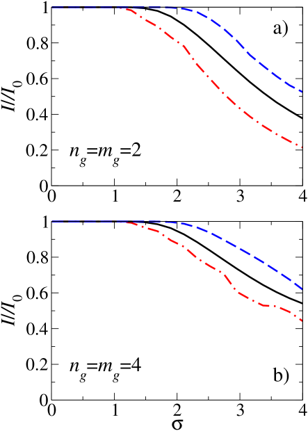
Figure 1: Clustering real value data: Mutual information $I=I(p^{O},p^{*})$ between the original $p^{O}$ and estimated $p^{*}$ groups assignments, relative to its maximum value $I_{0}$ when $p^{*}=p^{O}$. The original data was made of $n=100$ samples divided in $K$ groups and $m=100$ conditions divided in $L$ groups. The values of $X_{ij}$ were extracted from a normal distribution with mean $\mu_{kl}=k+l$ and variance $\sigma$. The figure shows the mutual information between the original groups and the group assignment, estimated by the VB-1 algorithm, as a function of the variance $\sigma$. The dashed-dotted, solid and dashed lines corresponds with the worst, average and best case on 100 test examples, respectively. In a) $K=L=2$ and in b) $K=L=4$. In both cases the mutual information is approximately equal to its maximum $I_{0}$ for values of $\sigma$ less than one, the minimum difference between the original means $\mu_{kl}$.

VI.2 Test examples

To test the performance of the VB-1 algorithm, (37)-(46), we consider test examples generated by the likelihood (33) itself. Our aim is to test the variational result in the context of a relatively small number of samples and conditions. To quantify the goodness of the group assignment we consider the mutual information between the original $p^{O}$ ($p^{O}_{ik}=\delta_{g_{i}k}$) and estimated $p^{*}$ sample group assignments,

$$I(p^{O},p^{*})=\sum_{kk^{\prime}}\rho_{kk^{\prime}}\ln\frac{\rho_{kk^{\prime}}}{\rho^{O}_{k}\rho^{*}_{k^{\prime}}}$$ (47)

where

$$\rho_{kk^{\prime}}=\frac{1}{n}\sum_{i}p^{O}_{ik}p^{*}_{ik}$$ (48)

$$\rho^{O}_{k}=\frac{1}{n}\sum_{i}p^{O}_{ik}$$ (49)

$$\rho^{*}_{k}=\frac{1}{n}\sum_{i}p^{*}_{ik}\ .$$ (50)

Note that $I(p^{O},p^{*})$ takes its maximum value when $p^{*}=p^{O}$, denoted by $I_{0}=I(p^{O},p^{O})$. Off course, the same could be done for the condition group assignments as well.

In our test examples the original data was made of $n=100$ samples divided in $K$ groups and $m=100$ conditions divided in $L$ groups. The values of $X_{ij}$ were extracted from a normal distribution with mean $\mu_{kl}=k+l$ and variance $\sigma$. We estimate the group assignment using the VB-1 algorithm, sampling one initial condition. Figure 1 shows the mutual information between the original and estimated groups as a function of the variance $\sigma$. In a) $K=L=2$ and in b) $K=L=4$. In both cases the mutual information is approximately equal to its maximum $I_{0}$ for values of $\sigma$ less than 1. Since 1 is the minimum difference between the original means $\mu_{kl}$, we conclude that the VB-1 algorithm performs well when there is a significant difference between the distributions associated with different groups. For larger values of $\sigma$ the VB-1 algorithm performance starts to decrease. This is not, however, a deficiency of the algorithm but an unavoidable consequence of the mixing between the distributions coming from different groups. It is worth noticing that we obtain similar results for the case $K=4$ and $L=1$, indicating that the method works when there is no group structure on one side, in this case the conditions.

VII Case study: clustering data represented by hypergraphs and bipartite graphs

There are several datasets consisting of a certain number of properties and the information of whether or not each sample exhibits each of the properties. For example, the dataset in Fig. 2 describes a population of three animals characterized by two attributes, hair and legs. The attribute hair can take the value YES (has hair) or NO (does not have hair) while the attribute legs takes the values 2 or 4 (at least within this dataset). The mathematical treatment of this problem is significantly simplified if the variables are mapped onto Boolean variables. To each $S$ states variable we associate $S$ Boolean variables, each representing the occurrence or not of a specific letter of the alphabet. For example, the attribute hair is associated with hair-YES and hair-NO and the attribute legs with legs-2 and legs-4 (Fig. 2b). The outcome of this mapping is represented by the Boolean matrix $a_{ij}$, taking the value 1 if the answer to the Boolean variable $j$ is YES on sample $i$ and 0 otherwise.

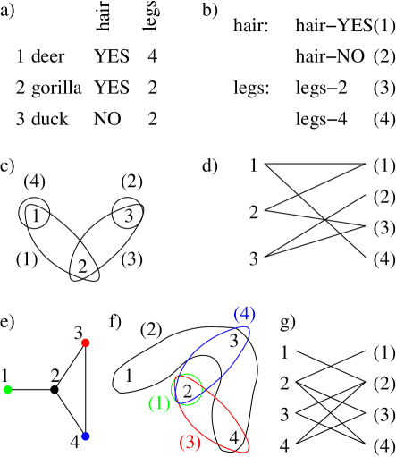
Figure 2: Hypergraph and bipartite graph data representations: a) An example of a problem with categorical data. b) Mapping of the categorical variables onto augmented Boolean variables. c) Hypergraph representation of the categorical dataset in a). d) Bipartite graph representation of the categorical dataset in a). e) A graph example. f) Nearest-neighbor mapping of the graph in e) onto a hypergraph, where each hyper-edge represents a set of nearest neighbors of a vertex in the original graph, indicated by (1), (2), (3) and (4). g) Nearest-neighbor mapping of the graph in e) onto a bipartite graph. The original graph vertices are represented by 1, 2, 3 and 4. The augmented bipartite graph vertices, representing nearest-neighbor sets, are represented by (1), (2), (3) and (4).

Depending on our aim, the Boolean matrix can be represented either by a hypergraph or a bipartite graph. When we aim to cluster the samples without attempting to cluster the Boolean variables, $a_{ij}$ is better interpreted as the adjacency matrix of a hypergraph. A hypergraph is an intuitive extension of the concept of graph to allow for connections between more than two elements. In our case, the hypergraph vertices represent samples and hyper-edges, one associated which each Boolean variable, represent the set of all samples with the answer YES to the corresponding Boolean variable (Fig. 2c). On the other hand, when we aim to cluster both the samples and Boolean variables then a bipartite graph interpretation is more appropriate, with one class of vertices for the samples and another one for the Boolean variables, and an edge connecting sample $i$ and variable $j$ whenever $a_{ij}=1$ (2d). The differences between these two approaches will become clear below.

VII.1 One side clustering: Statistical model on hypergraphs

In this case the samples are assumed to be divided in groups while the hypergraph edges are modeled as independent. Here we follow the statistical model introduced in Vazquez :

Data: Consider a hypergraph with a vertex set representing $n$ samples and $m$ edges characterizing the relationships among them. The hypergraph is specified by its adjacency matrix $a$, where $a_{ij}=1$ if element $i$ belongs to edge $j$ and it is 0 otherwise.

Likelihood: The adjacency matrix elements are generated by a binomial model with sample group and variable dependent probabilities $\theta_{kj}$, $k=1,\ldots,K$ and $j=1,\dots,m$, resulting in

$$P(a|g,\theta)=\prod_{ij}\theta_{g_{i}j}^{a_{ij}}\left(1-\theta_{g_{i}j}\right)^{1-a_{ij}}\ ,$$ (51)

Priors: As priors we use the renormalized invariant prior of the binomial model (Table 1). Taking into account that we have a binomial model for each pair of sample group and edge, we obtain

$$P(\theta)=\prod_{kj}{\rm Beta}(\theta_{kj};\tilde{\alpha}_{kj},\tilde{\beta}_{kj})$$ (52)

with $\tilde{\alpha}_{kj}\rightarrow 0$ and $\tilde{\beta}\rightarrow 0$.

Substitute the likelihood (51), the priors (29) and (52), and the MF variational function (31) into (5), and integrating over $\phi$ (summing over $g_{i}$ and integrating over $\theta_{kl}$ and $\pi_{k}$) we obtain

$$F \leq -\sum_{jk}\left(\sum_{i}p_{ik}a_{ij}+\tilde{\alpha}_{kj}-1\right)\langle\ln\theta_{kj}\rangle$$ (53)

$$- \sum_{jk}\left(\sum_{i}p_{ik}(1-a_{ij})+\tilde{\beta}_{kj}-1\right)\langle\ln(1-\theta_{kj})\rangle$$

$$+ \sum_{ik}p_{ik}\ln p_{ik}+\int d\theta R(\theta)\ln R(\theta)$$

$$+ \int d\pi R(\pi)\ln R(\pi)+{\rm const.}$$

Minimizing (53) with respect to $p_{il}$, $R(\theta)$ and $R(\pi)$ we obtain (VB-2)

$$p_{ik}=\frac{e^{\langle\ln\pi_{k}\rangle+\sum_{j}\left[a_{ij}\langle\ln\theta_{kj}\rangle+(1-a_{ij})\langle\ln(1-\theta_{kj})\rangle\right]}}{\sum_{s}e^{\langle\ln\pi_{s}\rangle+\sum_{j}\left[a_{ij}\langle\ln\theta_{sj}\rangle+(1-a_{ij})\langle\ln(1-\theta_{sj})\rangle\right]}}$$ (54)

$$R(\theta)=\prod_{kj}{\rm B}(\theta_{kj};\alpha_{kj},\beta_{kj})\ ,$$ (55)

$$\alpha_{kj}=\tilde{\alpha}_{kj}+\sum_{ij}p_{ik}a_{ij}$$ (56)

$$\beta_{kj}=\tilde{\beta}_{kj}+\sum_{ij}p_{ik}(1-a_{ij})\ .$$ (57)

$$R(\pi)={\rm D}(\pi;\gamma)\ ,\ \ \ \ \gamma_{k}=\tilde{\gamma}_{k}+\sum_{i}p_{ik}$$ (58)

$$F^{*} = {\rm const.}+\sum_{ik}p_{ik}\ln p_{ik}$$ (59)

$$- \sum_{kj}\ln{\rm B}(\alpha_{kj},\beta_{kj})-\ln{\rm B}(\gamma)$$

These equations represent the VB algorithm for the statistical model on hypergraphs. In this case we have not been able to disentangle the contributions weighting the fit to the data and the model bias, both being included in the averages $\langle\ln(\theta_{kj})\rangle$ and $\langle\ln(1-\theta_{kj})\rangle$.

VII.2 VB algorithm implementation, statistical model on hypergraphs

The implementation of the VB algorithm for the statistical model on hypergraphs proceeds as follows. Set sufficiently large values for $K$, larger than our expectation for the actual values of $K$. We use $K=20$ in the following test examples. Set the parameters $\tilde{\alpha}_{kj}$, $\tilde{\beta}_{kj}$ and $\tilde{\gamma}_{k}$. We set the parameters $\tilde{\alpha}_{kj}=\tilde{\beta}_{kj}=\tilde{\gamma}_{k}=10^{-6}$. Set random initial conditions for $p_{ik}$. Starting from these initial conditions iterate equations (54)-(59) until the solution converges up to some predefined accuracy. We use relative error of $F^{*}$ smaller than $10^{-6}$. In practice, compute $\alpha_{kj}$, $\beta_{kj}$, $\langle\ln\theta_{kj}\rangle$, $\langle\ln(1-\theta_{kj})\rangle$, $\gamma_{k}$, $\langle\ln\pi_{k}\rangle$, $p_{ik}$ and $F^{*}$ in that order. To explore different potential local minima use different initial conditions and select the solution with lowest $F^{*}$. Since this algorithm penalizes groups with few members it turns out that, for sufficiently large $K$, some sample and condition groups result empty. If this is not the case then increase $K$ until at least one group is empty. A matlab code implementing this algorithm can be found at http://www.sns.ias.edu/ vazquez/hgc.html.

Figure 3: Stratification or an animal population: a) A list of animals is given together with certain attributes characterizing them. The complete dataset is available from Asuncion and Newman (2007). Except for the attribute - legs - one and zero indicate possession or not, respectively, of the corresponding attribute. The problem consist on determining the optimal stratification of the animal population based on the provided attributes. b) Hypergraph representing the zoo data. Each line corresponds with an edge, whose elements are specified within the right column. c) Stratification as obtained in Vazquez . d) Stratification by the VB-2 algorithm. e) and f) Stratification of the animal population e) and Boolean variables f) by the VB-3 algorithm.

VII.2.1 Test example: zoo problem

Consider the animal population in Fig. 3a together with their attributes: habitat, nutrition behavior, etc. Figure 3b shows the mapping of this dataset onto a hypergraph. The hypergraph vertices represent animals and the edges represent the association between all animals with a given attribute: edge 1, all non-airborne animals; edge 2, all airborne animals, and so on.

The animal population stratification was already addressed in Vazquez , finding the solution in Fig. 3c. Although the starting statistical model is the same, the solution in Vazquez was found assuming fixed the number of groups and estimating the group assignment using the EM algorithm (essentially a maximum likelihood estimate). Then, in an an attempt to focus in the solution with better consensus, solutions for different number of groups were obtained and the most representative solution was selected.

Here we address the same problem using a Bayesian approach and the variational solution. We start from the same statistical model on hypergraphs but now obtain a solution using the VB-2 algorithm (54)-(59), sampling 10,000 initial conditions as in Vazquez . The solution found by the VB-2 algorithm (Fig. 3d) is quite similar to that previously found in Vazquez (Fig. 3c). The main differences are the splitting of the terrestrial mammals, the exclusion of the platypus and the tortoise from the amphibia-reptiles group and the scorpion from the terrestrial arthropods. More important, in both cases the main groups represent terrestrial mammals, aquatic mammals, birds, fishes, amphibia-reptiles, terrestrial arthropods and aquatic arthropods. The VB-2 (54)-(53) algorithm represents, however, a significant improvement over the approach followed in Vazquez . It finds the consensus solution in one run, because it has built in the balance between better fitting and less bias.

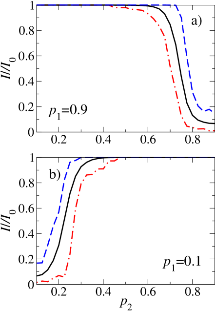
Figure 4: Finding graph modules, hypergraph model: Mutual information $I=I(p^{O},p^{*})$ between the original $p^{O}$ and estimated $p^{*}$ groups assignments, relative to its maximum value $I_{0}$ when $p^{*}=p^{O}$. The original data was made of a graph with $n=100$ vertices divided in $K=2$ groups, with an intra- and inter-community connection probabilities $p_{1}$ and $p_{2}$, respectively. The figure shows the mutual information, between the original groups and the group assignment estimated by the VB-2 algorithm (54)-(59), as a function of the inter-community connectivity $p_{2}$. The dashed-dotted, solid and dashed lines corresponds with the worst, average and best case on 100 test examples. In a) we deal with dense communities ($p_{1}=0.9$) and the algorithm performs well ($I/I_{0}\approx 1$) for small values of the inter-community connectivity probability $p_{2}$. In b) we deal with sparse communities ($p_{1}=0.1$) and the algorithm performs well for large values of the inter-community connectivity probability $p_{2}$.

VII.2.2 Test example: finding network modules

The work by Newman and Leicht Newman and Leicht (2007) provides a hint on how to apply the hypergraph clustering to the problem of finding modules or communities in a graph or network. A graph is made by a set of vertices and a set of edges, the latter being pairs of connected vertices. The idea of Leicht and Newman is a “guilty by association” principle: vertices between the same module of a graph will tend to have connections to the same other vertices. This problem can be translated to a hypergraph problem, where the vertices are the graphs vertices, the hyper-edges are the set of nearest neighbors and the Boolean variables characterize whether or not a vertex belongs to the a set of nearest neighbors Vazquez (Fig. 2e and f). More precisely, to each vertex we associate a hyper-edge, given by the set of its nearest neighbors. Therefore, there are $m=n$ hyper-edges, one for every vertex in the original graph. The hypergraph adjacency matrix has the matrix element $a_{ij}=1$ if vertex $i$ belongs to hyper-edge $j$, i.e. if vertex $i$ belongs to the nearest-neighbor set of vertex $j$, and $a_{ij}=0$ otherwise. If we label the nearest-neighbor sets with the same label as the vertices then the hypergraph adjacency matrix coincides with the adjacency matrix of the original graph. Thus, there is an exact mapping from the statistical model proposed by Newman and Leicht Newman and Leicht (2007) to the statistical model on hypergraphs.

Having specified this mapping we use the VB-2 algorithm (54)-(59), sampling one initial condition, to find the graph modules in the original graph. To illustrate its performance we consider as a case study a graph composed by two communities, with probabilities $p_{1}$ and $p_{2}$ that two vertices within the same or different communities are connected, respectively. As already anticipated by Newman and Leicht Newman and Leicht (2007), the nearest-neighbor approach can resolve both dense communities with lesser inter-community connections ($p_{1}\gg p_{2}$) and sparse communities with more inter-community connections ($p_{1}\ll p_{2}$). Figure 4 shows that the VB-2 algorithm performs quite well in those two regimes.

VII.3 Two sides clustering: statistical model on bipartite graphs

We can face situations where there are groups of Boolean variables as well, requiring the clustering of both samples and Boolean variables. In this case the bipartite graph representation is more appropriate, with a class of vertices representing the samples and a class of vertices representing the Boolean variables. More precisely,

Data: Consider a bipartite graph with two vertex subsets, representing $n$ samples and $m$ Boolean variables. The graph is specified by its adjacency matrix $a$, where $a_{ij}=1$ when sample $i$ is connected to Boolean variable $j$, i.e. if Boolean variable $j$ is true for sample $i$, and $a_{ij}=0$ otherwise.

Likelihood: The adjacency matrix elements are generated by a binomial model with sample group and variable group dependent probabilities $\theta_{kl}$, $k=1,\ldots,K$ and $l=1,\dots,L$, resulting in

$$P(a|g,c,\theta)=\prod_{ij}\theta_{g_{i}c_{j}}^{a_{ij}}\left(1-\theta_{g_{i}c_{j}}\right)^{1-a_{ij}}\ .$$ (60)

Priors: For $P(\theta)$ we use the renormalized invariant prior of the binomial model. Taking into account that we have one binomial model per each pair of sample and variable group we obtain

$$P(\phi)=\prod_{kj}{\rm B}(\theta_{kl};\tilde{\alpha}_{kl},\tilde{\beta}_{kl})$$ (61)

with $\tilde{\alpha}_{kl}\rightarrow 0$ and $\tilde{\beta}_{k}\rightarrow 0$.

The likelihood (60) is quite similar to (51), the main difference being that now the statistical properties of the Boolean variables appear through their corresponding group assignments $c_{j}$. This increases the model complexity by considering a group structure for the Boolean variables and, at the same time, reduces the number of $\theta$ parameters. Furthermore, (60) contains (51) as the particular case where $L=n$ and one group associated to each Boolean variable.

Substituting the likelihood (60), the priors (61), (29) and (30), and the MF variational function (32) in (5), and integrating over $\phi$ (summing over $g_{i}$ and $c_{j}$ and integrating over $\theta_{kl}$, $\pi_{k}$ and $\kappa_{l}$) we obtain

$$F \leq -\sum_{kl}\left(\sum_{ij}p_{ik}q_{jl}a_{ij}+\tilde{\alpha}_{kl}-1\right)\langle\ln\theta_{kl}\rangle$$ (62)

$$+ \sum_{kl}\left(\sum_{ij}p_{ik}q_{jl}(1-a_{ij})+\tilde{\beta}_{kl}-1\right)\langle\ln(1-\theta_{kl})\rangle$$

$$+ \sum_{ik}p_{ik}\ln p_{ik}+\sum_{jl}q_{jl}\ln q_{jl}$$

$$+ \int d\theta R(\theta)\ln R(\theta)+\int d\pi R(\pi)\ln R(\pi)$$

$$+ \int d\kappa R(\kappa)\ln R(\kappa)+{\rm const.}$$

Minimizing (62) with respect to $p_{il}$, $q_{jl}$, $R(\theta)$, $R(\pi)$ and $R(\kappa)$ we obtain (VB-3)

$$p_{ik}=\frac{e^{\langle\pi_{k}\rangle+\sum_{jl}q_{jl}\left[a_{ij}\langle\ln\theta_{kl}\rangle+(1-a_{ij})\langle\ln(1-\theta_{kl})\rangle\right]}}{\sum_{s}e^{\langle\pi_{s}\rangle+\sum_{jl}q_{jl}\left[a_{ij}\langle\ln\theta_{sl}\rangle+(1-a_{ij})\langle\ln(1-\theta_{sl})\rangle\right]}}$$ (63)

$$q_{jl}=\frac{e^{\langle\kappa_{l}\rangle+\sum_{ik}p_{ik}\left[a_{ij}\langle\ln\theta_{kl}\rangle+(1-a_{ij})\langle\ln(1-\theta_{kl})\rangle\right]}}{\sum_{s}e^{\langle\kappa_{s}\rangle+\sum_{ik}p_{ik}\left[a_{ij}\langle\ln\theta_{ks}\rangle+(1-a_{ij})\langle\ln(1-\theta_{ks})\rangle\right]}}$$ (64)

$$R(\theta)=\prod_{kl}{\rm B}(\theta_{kl};\alpha_{kl},\beta_{kl})\ ,$$ (65)

$$\alpha_{kl}=1+\sum_{ij}p_{ik}q_{jl}a_{ij}$$ (66)

$$\beta_{kl}=1+\sum_{ij}p_{ik}q_{jl}(1-a_{ij})\ .$$ (67)

$$R(\pi)={\rm D}(\pi;\gamma)\ ,\ \ \ \ \gamma_{k}=\tilde{\gamma}_{k}+\sum_{i}p_{ik}$$ (68)

$$R(\pi)={\rm D}(\kappa;\epsilon)\ ,\ \ \ \ \epsilon_{l}=\tilde{\epsilon}_{l}+\sum_{j}q_{jl}$$ (69)

$$F^{*} = {\rm const.}+\sum_{ik}p_{ik}\ln p_{ik}+\sum_{jl}q_{jl}\ln q_{jl}$$ (70)

$$- \sum_{kl}\ln{\rm B}(\alpha_{kl},\beta_{kl})-\ln{\rm B}(\gamma)-\ln{\rm B}(\epsilon)$$

Equations (63)-(70) represent the VB algorithm for the statistical model on bipartite graphs. They can be used to found modules or communities in graphs with a bipartite structure, including those representing samples and Boolean variables.

VII.4 VB algorithm implementation, statistical model on bipartite graphs

The implementation of the VB-2 algorithm (63)-(70) for the statistical model on bipartite graphs proceeds as follows. Set sufficiently large values for $K$ and $L$, larger than our expectation for the actual values of $K$ and $L$. Set the parameters $\tilde{\alpha}_{kl}$, $\tilde{\beta}_{kl}$, $\tilde{\gamma}_{k}$ and $\tilde{\epsilon}_{l}$. We set the parameters $\tilde{\alpha}_{kl}=\tilde{\beta}_{kl}=\tilde{\gamma}_{k}=\tilde{\epsilon}_{l}=10^{-6}$. Set random initial conditions for $p_{ik}$ and $q_{jl}$. Starting from these initial conditions iterate equations (63)-(70) until the solution converges up to some predefined accuracy. We use relative error of $F^{*}$ smaller than $10^{-6}$. In practice, compute $\alpha_{kj}$, $\beta_{kj}$, $\langle\ln\theta_{kj}\rangle$, $\langle\ln(1-\theta_{kj})\rangle$, $\gamma_{k}$, $\langle\ln\pi_{k}\rangle$, $\epsilon_{l}$, $\langle\ln\kappa_{l}\rangle$, $p_{ik}$, $q_{jl}$ and $F^{*}$ in that order. To explore different potential local minima use different initial conditions and select the solution with lowest $F^{*}$. Since this algorithm penalizes groups with few members it turns out that, for sufficiently large $K$ and $L$ some sample and/or variable groups result empty. If this is not the case, increase $K$ and/or $L$ until at least one sample group and one variable group results empty.

VII.4.1 Test example: zoo problem

Let us go back to the zoo problem (Fig. 3a). Now we represent this dataset by a bipartitite graph, with one class of vertices representing the animals and the other class the Boolean variables (e.g. Fig. 2a,b and d) Using the VB-3 algorithm (63)-(70), sampling 10,000 initial conditions as in Vazquez , we perform a two-sides clustering of the bipartite graph obtaining the animal population stratification in Fig. 3e and the Boolean variables stratification in Fig. 3f. The animal clusters are similar to those previously obtained using the statistical model on hypergraphs (Fig. 3c and d). The main difference is the more refined subdivision of terrestrial mammals, now split in four groups (1, 2, 3 and 4).

In addition to the animal population stratification the two-sides clustering provides association groups between the Boolean variables (Fig. 3f). These associations reflect the fact that not all Boolean variables are independent, some of them are linked. For example, group 2 cluster four typical attributes of terrestrial mammals, they have hair, do not put eggs, milk and have four legs. In the same way, group 3 clusters attributes of fishes and group four of birds. Thus, in general, the bipartite graph model and the resulting two-sides clustering provides more information than the hypergraph approach.

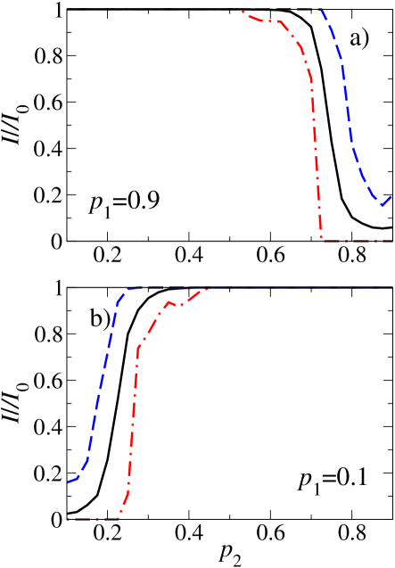
Figure 5: Finding graph modules, bipartite model: Mutual information $I=I(p^{O},p^{*})$ between the original $p^{O}$ and estimated $p^{*}$ groups assignments, relative to its maximum value $I_{0}$ when $p^{*}=p^{O}$. The original data was made of a graph with $n=100$ vertices divided in $K=2$ groups, with an intra and inter-community connection probabilities $p_{1}$ and $p_{2}$, respectively. The figure shows the mutual information, between the original groups and the group assignment estimate by the VEM-3 algorithm (63)-(70), as a function of the inter-community connectivity $p_{2}$. The dashed-dotted, solid and dashed lines corresponds with the worst, average and best case on 100 test examples. In a) we deal with dense communities ($p_{1}=0.9$) and the algorithm performs well ($I/I_{0}\approx 1$) for small values of the inter-community connectivity probability $p_{2}$. In b) we deal with sparse communities ($p_{1}=0.1$) and the algorithm performs well for large values of the inter-community connectivity probability $p_{2}$.

VII.4.2 Test example: finding network modules

The bipartite graph model can be use to find network modules as well. In this case one class of vertices represents the original graph vertices and the other represents sets of nearest neighbors (Fig. 2g). The two-sides clustering thus attempts to cluster both the original graph vertices and the sets of nearest neighbors. When the original graph is undirected the problem is symmetric (e.g. see Fig. 2g). Indeed, if vertex $i$ belongs to the nearest-neighbor set of vertex $j$ then vertex $j$ belongs to the nearest-neighbor set of vertex $i$. As a consequence the clustering on the original vertices side cannot be differentiated from the clustering of nearest-neighbor sets. Intuitively this means that when two vertices belong to the same graph module we can say that their nearest-neighbor sets belong to the same nearest-neighbor set group.

Having specified this mapping we use the VB-3 algorithm (63)-(70), sampling one initial condition, to find the graph modules in the original graph. To illustrate its performance we consider once again a graph composed by two communities, with probabilities $p_{1}$ and $p_{2}$ that two vertices within the same or different communities are connected, respectively. Figure 5 shows that the VB-3 algorithm can resolve both dense communities with lesser inter-community connections ($p_{1}\gg p_{2}$) and sparse communities with more inter-community connections ($p_{1}\ll p_{2}$).

The comparison of Fig. 5 and 4 indicates that the bipartite graph model performs slightly better than the hypergraph model. For example, focusing on the average performance, for $p_{1}=0.9$ the VB-3 algorithm performs almost perfectly till $p_{2}=0.6$, while the VB-2 algorithm does till $p_{2}=0.5$. This could be, however, specific to the tested set of examples. Further research is required to determine which version performs better depending on the dataset under consideration.

VIII Discussion and conclusions

The Bayesian approach allows for a systematic solution of data analysis problems. Its starting point is a statistical model of the data under consideration. From there, using Bayes rule, we can invert the statistical model to obtain the posterior distribution of the model parameters. The latter can be use, in principle, to calculate or compute averages or other magnitudes of interest.

One of the main criticisms to the Bayesian approach is the apparent ambiguity in selecting the prior distributions. Here we have worked further on Jaynes method Jaynes (1969), claiming that the prior distributions are given by the most general distribution dictated by the symmetries of the problem under consideration. One undesired consequence of this method is that when the symmetries are not sufficient constraints we obtain improper prior distributions. Yet, the use of improper priors can be avoided by working with renormalized distributions that are proper, and approach the improper prior in a certain limit. Using this approach we report here a correction to Jaynes prior for a likelihood with translation and scale invariance and a generalization of Jaynes prior for the binomial model to the multinomial model.

Having resolve the issue about the prior distributions, we can proceed to the application of the Bayesian approach to resolve a population structured. Taking inspiration from mixture models McLachlan and Peel (2000), in particular Dirichlet mixture models Blei et al. (2003), we introduce general statistical models with a built in population structure at the sample, and sample and variable, level. The model with a structure at the sample level aims one-side clustering problems, where the variables are assumed to be independent measurements. The model with a structure at both sample and variable level aims two-side clustering problems, where there are classes of variables. These statistical models are then postulated as generative models of some dataset. Introducing a MF approximation as variational function, we then resolve the population structure by solving the inverse problem, i.e. determining the sample and/or variable groups and model parameters from the data.

To illustrate the applicability and systematicity of the variational method, here we study the problem of data clustering, in the context of real value and Boolean variables. The outcome is a variational Bayes (VB) algorithm, a self-consistent set of equations to determine the group assignments and the model parameters. The VB algorithm is based on recursive equations similar to those for the EM algorithm, but with some intrinsic penalization for model bias. In the case of real value data, and under the assumption of normal distributions, the contributions favoring fitting and penalizing model bias are clearly disentangled. The fitting is quantified, as it is expected for normally distributed variables, by the mean square deviation. The model bias is quantified by the inverse of the square root of the mean cluster sizes. The tendency to reduce the mean square deviation is thus balanced by a tendency to increase the cluster sizes.

In the case of Boolean variables our analysis is based on a mapping into a hypergraph or bipartite graph. When we cluster the samples but not the Boolean variables the problem is mapped onto a statistical model on hypergraphs Vazquez . On the other hand, when we perform a two-side clustering, clustering both the samples and the Boolean variables, the problem is mapped onto a statistical model on bipartite graphs.

The VB algorithms associated with the statistical model on hypergraphs and bipartite graphs can be used to find modules on a graph. Starting on an idea by Newman and Leicht Newman and Leicht (2007), we show that the problem of graph modules can be mapped onto the problem of finding hypergraph modules or bipartite graph modules, where the hypergraph edges and the augmented bipartite graph vertices represent nearest-neighbor sets in the original graph. The resulting VB algorithms represent a significant improvement over the maximum likelihood approaches followed in Newman and Leicht (2007) and Vazquez , by including a self-consistent correction for model complexity and bias.

It is worth mentioning that, depending on the starting statistical model, we could arrive to different versions of the VB algorithm. Indeed, for the finding graph modules problem we could use both the hypergraph and bipartite graph models. Furthermore, Hofman and Wiggins Hofman and Wiggins have obtained another version based on a statistical model with different intra and inter-community connection probabilities. These approaches differ in the definition of what constitutes a group, community or module. We use the definition by Newman and Leicht Newman and Leicht (2007) based on topological similarity, i.e. two vertixes are topologically identical if they are connected to the same other vertices in the graph. Thus, we obtain group of vertices whose patterns of connectivity are similar. On the other hand, the definition used by Hofman and Wiggins Hofman and Wiggins is based on the existence of two edge densities, characterizing the tendency of having an edge between intra- and inter-group pairs of vertices. Depending on the problem and the question we are asking we may adopt one or the other definition, and use the corresponding clustering method.

References

- McLachlan and Peel (2000) G. McLachlan and D. Peel, Finite Mixture Models (John Wiley & Sons, Inc., New York, 2000).
- Dempster et al. (1977) A. Dempster, N. Laird, and D. Rubin, J R Statisti Soc B 39, 1 (1977).
- Akaike (1974) H. Akaike, IEEE Trans. Aut. Control 19, 716 (1974).
- Schwarz (1978) G. Schwarz, Ann. Statist. 6, 461 (1978).
- Jeffreys (1939) H. Jeffreys, Theory of Probability (Oxford, University Press, OXford, 1939).
- Spirtes et al. (2000) P. Spirtes, C. Glymour, and R. Scheines, Causation, prediction, and search (MIT Press, Cambridge, 2000).
- MacKay (2003) D. J. C. MacKay, Information theory, inference, and learning algorithms (Cambridge University Press, Cambridge, 2003).
- Robert (2007) C. P. Robert, The Bayesian choice (Springer, New York, 2007).
- Chen et al. (2000) M.-H. Chen, Q.-M. Shao, and J. G. Ibrahim, Monte Carlo methods in Bayesian Computation (Springer-Verlag, New York, 2000).
- (10) M. J. Beal, phD. Thesis, Gatsby Computational Neuroscience Unit, University College London, 2003.
- Yedidia et al. (2005) J. S. Yedidia, W. T. Freeman, and Y. Weiss, IEEE Trans Inf Theor 51, 2282 (2005).
- Rasmussen (2000) C. E. Rasmussen, Adv. Neural Inf. Proc. Syst. 12, 554 (2000).
- Blei et al. (2003) D. M. Blei, A. Y. Ng, and M. I. Jordan, J. Machine Learn Res 3, 993 (2003).
- (14) J. M. Hofman and C. H. Wiggins, arXiv:0709.3512v2 [physics.data-an].
- Jaynes (1969) E. T. Jaynes, IEEE Trans. Syst. Sci. and Cybernet. SSC-4, 227 (1969).
- Kullback (1959) S. Kullback, Information Theory and Statistics (Wiley, New York, 1959).
- (17) A. Vazquez, phys. Rev. E (In press); arXiv:0712.1365v1 [q-bio.PE].
- Asuncion and Newman (2007) A. Asuncion and D. Newman, UCI machine learning repository (2007), URL http://www.ics.uci.edu/~mlearn/MLRepository.html.
- Newman and Leicht (2007) M. Newman and E. Leicht, Proc. Natl. Acad. Sci. USA 104, 564 (2007).