Pions in the quark matter phase diagram

Abstract

The relationship between mesonic correlations and quantum condensates in the quark matter phase diagram is explored within a quantum field theoretical approach of the Nambu and Jona-Lasinio (NJL) type. Mean-field values in the scalar meson and diquark channels are order parameters signalling the occurrence of quark condensates, entailing chiral symmetry breaking ($\chi$SB) and color superconductivity (2SC) in quark matter. We investigate the spectral properties of scalar and pseudoscalar meson excitations in the phase diagram in Gaussian approximation and show that outside the $\chi$SB region where the pion is a zero-width bound state, there are two regions where it can be considered as a quasi-bound state with a lifetime exceeding that of a typical heavy-ion collision fireball: (A) the high-temperature $\chi$SB crossover region at low densities and (B) the high-density color superconducting phase at temperatures below 100 MeV.

1 Introduction

The study of the QCD phase diagram is a key issue in modern theoretical and experimental physics of dense matter. Recent heavy-ion collision experiments at RHIC Brookhaven Muller:2006ee have led to the insight that the quark-gluon plasma (QGP) at high temperatures behaves as a perfect fluid with a low viscosity to entropy ratio $\eta/s\approx 0.1-0.2$ Shuryak:2003xe ; Shuryak:2003ty ; Teaney:2004qa which is very close to the KSS bound KSS for this number, $1/(4\pi)$. This strong deviation from the behavior of a gas of weakly interacting quarks and gluons is attributed to the occurence of mesonic bound states Shuryak:2003xe ; Shuryak:2003ty ; Shuryak:2004tx or resonances Blaschke:2003ut ; Blaschke:2005cm ; Abuki:2006dv in the strongly coupled QGP (sQGP). It has been pointed out Shuryak:2006ap that this situation in hot and dense QCD matter bears similarities with strongly coupled plasmas in other systems where bound state dissociation or Mott-Anderson delocalization Mott occurs since the effective coupling strength is modified by electronic screening and/or Pauli blocking effects. It is thus a very general effect expected to occur in a wide variety of dense Fermi systems with attractive interactions Armen:2006 ; Bronold:2006 ; Redmer:2006 ; Schmidt:1990 ; Stein:1995 ; Schnell:1999tu ; Kitazawa:2001ft ; Kitazawa:2003cs ; Blaschke:2004cs ; Blaschke:2005uj . When this Mott transition from truly bound to resonantly paired states occurs under conditions of Bose condensation one speaks of a BEC-BCS crossover chenfig ; Calzetta:2006 ; Gurarie:2007 . Recently, this transition became accessible to laboratory experiments with ultracold gases of fermionic atoms coupled via Feshbach resonances with a strength tunable by applying external magnetic fields Gurarie:2007 ; greiner:2003 ; Zwierlein:2003 ; Zwierlein:2005 ; Greiner:2003a . The BEC-BCS crossover transition in quark matter is of particular theoretical interest due to the additional relativistic regime it offers Abuki:2006dv ; Deng:2006ed ; Sun:2007fc .

Theoretical concepts explaining the appearance of nonperturbative phenomena like quantum condensates and bound states in dense Fermi systems with their observable consequences shall apply here but must be formulated within a quantum field theoretic approach. A systematic treatment of these effects is possible within the path integral formulation for finite-temperature quantum field theories. This approach is especially suited to take into account the effects of spontaneous symmetry breaking. Here we will apply this approach on the example of a model field theory of the NJL type to quark matter as a relativistic strongly interacting Fermi system. It is our aim to delineate relationships between the regions of the NJL model phase diagram where $\chi$SB and color superconductivity occur and the possibility to observe quasi-bound pionic states in HIC experiments where hot, dense QCD matter produced in the form of rather short-lived fireballs.

2 Scalar-pseudoscalar mesons in a superconducting two-flavor NJL model

As a generic model system for the description of hot, dense Fermi-systems with strong, short-range interactions we consider quark matter described by a model Lagrangian with four-fermion coupling. The key quantity is the partition function $\mathcal{Z}$ from which all thermodynamic quantities can be derived. In the imaginary time formalism (${t=-i\tau}$) it can be expressed as a path integral Kapusta:1989

$$\mathcal{Z}=\int\mathcal{D}(iq^{\dagger})\mathcal{D}(q)\;e^{\int^{\beta}\,d^{4}x\,(\mathcal{L}-\mu q^{\dagger}q)}~{},$$ (1)

where the chemical potential $\mu$ is introduced as a Lagrange multiplier for assuring conservation of baryon number. The notation $\int^{\beta}\,d^{4}x$ is shorthand for $\int_{0}^{\beta}\,d\tau\int\,d^{3}x$ where $\beta$ is the inverse temperature. The quark matter is described by a Dirac Lagrangian with internal degrees of freedom ($N_{f}=2$ flavors , $N_{c}=3$ colors), with a current-current-type four-fermion interaction inspired by one-gluon exchange. After Fierz transformation of the interaction, we select the scalar diquark channel and the scalar-pseudoscalar meson channels so that our model Lagrangian assumes the form

$$\mathcal{L}=\bar{q}(i\not{\partial}-m_{0})q+G_{D}(\bar{q}i\gamma_{5}C\tau_{2}\lambda_{2}\bar{q}^{T})(q^{T}iC\gamma_{5}\tau_{2}\lambda_{2}q)+G_{S}\big{[}\left(\bar{q}q\right)^{2}+\left(\bar{q}i\gamma_{5}{\bf\tau}q\right)^{2}\big{]}~{}.$$ (2)

Here $\gamma_{\nu}$ are the Dirac matrices, $\lambda_{2}$ is a color $SU(3)$ Gell-Mann matrix, $\tau_{i}$ are $SU(2)$ flavor matrices and $C=i\gamma^{2}\gamma^{0}$ is the charge conjugation matrix. $G_{S}$ and $G_{D}$ are coupling strengths corresponding to the different channels, see Ref. Buballa:2003qv for a recent review. For the numerical analysis we adopt parameters from Ref. Grigorian:2006qe and consider $G_{D}$ as a free parameter.

After introduction of the Hubbard-Stratonovich Kleinert:1977tv auxiliary fields $\Delta(\tau,x)$, $\Delta^{*}(\tau,x)$, $\pi(\tau,x)$, $\sigma(\tau,x)$ and the Nambu-Gorkov spinors $\Psi=\frac{1}{\sqrt{2}}(qq^{c})^{T}$, $\bar{\Psi}=\frac{1}{\sqrt{2}}(\bar{q}\bar{q}^{c})$ with $q^{c}(x)\equiv C\bar{q}^{T}(x)$, the partition function becomes a Gaussian path integral in the bispinor fields which can be evaluated and yields the fermion determinant

$$\mathcal{Z} = \int\mathcal{D}\Delta^{*}\mathcal{D}\Delta\mathcal{D}\sigma\mathcal{D}\pi e^{-\int^{\beta}d^{4}x\frac{\sigma^{2}+\pi^{2}}{4G_{S}}+\frac{|\Delta|^{2}}{4G_{D}}}\cdot{\rm Det}[S^{-1}]~{},$$ (3)

where the inverse bispinor propagator is a matrix in Nambu-Gorkov-, Dirac-, color- and flavor space. After Fourier transformation it reads

$$S^{-1} = \left(\begin{array}[]{cc}(i\omega_{n}+\mu)\gamma_{0}-m-i{\bm{\gamma}}\cdot{\bf p}-i\gamma_{5}{\bm{\tau}}\cdot{\bm{\pi}}&i\Delta\gamma_{5}\tau_{2}\lambda_{2}\\ i\Delta^{*}\gamma_{5}\tau_{2}\lambda_{2}&(i\omega_{n}-\mu)\gamma_{0}-m-i{\bm{\gamma}}\cdot{\bf p}+i\gamma_{5}{\bm{\tau}}^{t}\cdot{\bm{\pi}}\end{array}\right)~{},$$ (6)

with $m=m_{0}+\sigma$. So far we could derive with (3) a very compact, bosonized form of the quark matter partition function (1) which is an exact transformation of (1), now formulated in terms of collective, bosonic fields. As we will demonstrate in the following, this form is suitable since it allows to obtain nonperturbative results already in the lowest orders with respect to an expansion around the stationary values of these fields. In performing this expansion, we may factorize the partition function into mean field (MF), Gaussian fluctuation (Gauss) and residual (res) contributions

$$Z(\mu,T)\equiv e^{-\beta\Omega(\mu,T)}=Z_{MF}(\mu,T)Z_{\rm Gauss}(\mu,T)Z_{\rm res}(\mu,T)~{}.$$

In the following we will discuss the physical content of these approximations. In thermodynamical equilibrium, the mean field values satisfy the stationarity condition that the thermodynamical potential $\Omega_{MF}\equiv-\frac{1}{\beta V}\ln\mathcal{Z}_{MF}$ be minimal, i.e. $\frac{\partial\Omega_{MF}}{\partial\sigma_{MF}}=\frac{\partial\Omega_{MF}}{\partial\pi_{MF}}=\frac{\partial\Omega_{MF}}{\partial\Delta_{MF}}=0~{}.$ This is equivalent to the fulfillment of the gap equations $\sigma_{MF}=-4G_{S}{\rm Tr}\left(S_{MF}\right)\equiv m-m_{0}$, ${\bm{\pi}}_{MF}=-4iG_{S}{\rm Tr}\left(\gamma_{5}{\bm{\tau}}S_{MF}\right)=0$ and $\Delta_{MF}=4G_{D}{\rm Tr}\left(\gamma_{5}\tau_{2}\lambda_{2}S_{MF}\right)=\Delta$, together with the stability criterion that the determinant of the curvature matrix formed by the second derivatives is positive. After the evaluation of the traces and the sum over the Matsubara frequencies one gets

$$\Omega_{MF} = -\frac{1}{\beta V}\ln\mathcal{Z}_{MF}=\frac{(m-m_{0})^{2}}{4G_{S}}+\frac{|\Delta|^{2}}{4G_{D}}-\frac{1}{\beta V}{\rm Tr}\left(\ln\beta S_{MF}^{-1}\right)$$ (7)

$$= \frac{(m-m_{0})^{2}}{4G_{S}}+\frac{|\Delta|^{2}}{4G_{D}}-4\int\frac{d^{3}p}{(2\pi)^{3}}\left[E_{\bf p}^{+}+E_{\bf p}^{-}+E_{\bf p}+2T\ln(1+e^{-\beta E_{\bf p}^{+}})\right.$$

$$+\left.2T\ln(1+e^{-\beta E_{\bf p}^{-}})+T\ln(1+e^{-\beta\xi_{\bf p}^{+}})+T\ln(1+e^{-\beta\xi_{\bf p}^{-}})\right]~{},$$

where we have defined the particle dispersion relation $E_{\bf p}^{\pm}=\sqrt{\left(\xi_{\bf p}^{\pm}\right)^{2}+\Delta^{2}}$ with $\xi_{\bf p}^{\pm}=E_{\bf p}\pm\mu$, $E_{\bf p}=\sqrt{m^{2}+{\bf p}^{2}}$. The $\Delta\neq 0$ dispersion law $E_{\bf p}^{-}$($E_{\bf p}^{+}$) is associated to the red and green quarks (antiquarks), whereas the ungapped blue quarks (antiquarks) have the dispersion $\xi^{-}_{\bf p}$ ($\xi^{+}_{\bf p}$). With the aformentioned stationarity conditions applied to Eq. (7) we obtain the gap equations for the order parameters $m$ and $\Delta$, which have to be solved self-consistently,

$$m-m_{0} = 8G_{S}m\,\int\frac{d^{3}p}{(2\pi)^{3}}\frac{1}{E_{\bf p}}\bigg{\{}\left[1-2n_{F}(E_{\bf p}^{-})\right]\frac{\xi_{\bf p}^{-}}{E_{\bf p}^{-}}$$ (8)

$$\hskip 42.67912pt+\left[1-2n_{F}(E_{\bf p}^{+})\right]\frac{\xi_{\bf p}^{+}}{E_{\bf p}^{+}}+n_{F}(-\xi_{\bf p}^{+})-n_{F}(\xi_{\bf p}^{-})\bigg{\}}~{},$$

$$\Delta = 8G_{D}\int\frac{d^{3}p}{(2\pi)^{3}}\left[\frac{1-2n_{F}(E_{\bf p}^{-})}{E_{\bf p}^{-}}+\frac{1-2n_{F}(E_{\bf p}^{+})}{E_{\bf p}^{+}}\right]~{}.$$ (9)

The Fermi distribution is $n_{F}(E)=(1+e^{\beta E})^{-1}$. Solutions of the gap equations for the dynamically generated quark mass $m$ and for the diquark pairing gap $\Delta$ at $T=0$ as a function of $\mu$ are shown in the left panel of Fig. 1.

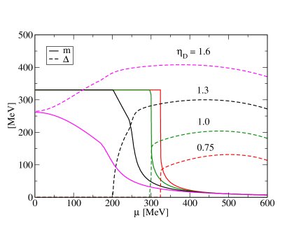
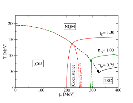
Figure 1: Left panel: order parameters for $\chi$SB (full lines) and color superconductivity (dashed lines) at $T=0$ for different values of $\eta_{D}$. First order phase transitions turn to second order or even crossover when $\eta_{D}$ is increased. For details, see text. Right panel: phase diagram of two-flavor quark matter with critical lines for chiral symmetry breaking (dashed) and color superconductivity (solid) for three values of the diquark coupling strength: $\eta_{D}=0.75$, $1.0$ and $1.3$. The dots indicate the critical endpoint for first order phase transitions.

From the solutions for the order parameters in dependence of the thermodynamical variables $T$ and $\mu$ we have constructed the phase diagram of the present quark matter model in the $T-\mu$ plane, see right panel of Fig. 1. The two order parameters, that are indicators of phase transitions, allow to distinguish 4 phases: $\Delta=0$, $m\sim m_{0}$: normal phase (NQM); $\Delta\neq 0$, $m\sim m_{0}$: color superconductor (2SC); $\Delta=0$, $m\gg m_{0}$: chiral symmetry broken phase ($\chi$SB); $\Delta\neq 0$, $m\gg m_{0}$: coexistence of $\chi$SB and 2SC phases.

Increasing the diquark coupling $\eta_{D}=G_{D}/G_{S}$ leads to an increase of the diquark gap and therefore a rise in the critical temperature for the second order transition to a normal quark matter phase. It shifts also the border between color superconductivity (2SC) and chiral symmetry broken phase ($\chi$SB) to lower values of the chemical potential. For very strong coupling $\eta_{D}\sim 1$, a coexistence region developes where both order parameters are simultaneously nonvanishing. Since the phase border is not of first order, no critical endpoint can be identified in this case. In the $\chi$SB phase pion and diquark exist as zero width bound states. At the chiral symmetry restoration transition, they merge the continuum of unbound states and turn into (resonant) scattering states. When this Mott transition occurs within the 2SC phase we speak of a BEC-BCS crossover.

Now we discuss the interesting question of the quasiparticle excitations in these phases. To this end, we will expand the action functional in the partition function up to quadratic order in the mesonic fields and arrive at a tractable approximation for the bosonized quark matter model.

Let us expand now the mesonic fields around their mean field values. In these lectures, we will focus on fluctuations in the mesonic channels, where the pion and the sigma meson will emerge as quasiparticle degrees of freedom. On the example of the pion we will explain the physics of the Mott transition. The detailed investigation of the quantized diquark fluctuations, which are also a prerequisite of the formation of baryons, will be given elsewhere Sun:2007fc ; Ebert:2004dr ; Anglani:2008 .

As mentioned above, the pion mean field vanishes, but the sigma field can be separated into mean field and fluctuations as $\sigma\rightarrow\sigma_{MF}+\sigma$. Hence it is possible to decompose the inverse propagator $S^{-1}$ into a mean field part and a fluctuation part $S^{-1}=S^{-1}_{MF}+\Sigma\,$, so that in the Gaussian approximation the fermion determinant becomes

$$\frac{{\rm Det}\left[S^{-1}\right]\big{|}_{\rm Gauss}}{{\rm Det}\left[S^{-1}_{MF}\right]}=\exp\left\{-\frac{1}{2}\int\frac{d^{4}q}{(2\pi)^{4}}{\rm Tr}\left[S_{MF}(p)\Sigma(q)S_{MF}(p+q)\Sigma(q)\right]\right\}~{},$$ (10)

where the matrix $\Sigma$ and the propagator $S_{MF}$ are defined as

$$\Sigma\equiv\left(\begin{array}[]{cc}-\sigma-i\gamma_{5}{\bm{\tau}}\cdot{\bm{\pi}}&0\\ 0&-\sigma-i\gamma_{5}{\bm{\tau}}^{t}\cdot{\bm{\pi}}\end{array}\right)\,,\;\;\;\;\;\;S_{MF}\equiv\left(\begin{array}[]{cc}{\bf G}^{+}&{\bf F}^{-}\\ {\bf F}^{+}&{\bf G}^{-}\end{array}\right)~{}.$$ (15)

The matrix elements of the Nambu-Gorkov propagator are

$${\bf G}^{\pm}_{p} = \sum_{s_{p}}\sum_{t_{p}}\frac{t_{p}}{2E_{\bf p}^{\pm s_{p}}}\frac{t_{p}E_{\bf p}^{\pm s_{p}}-s_{p}\xi_{\bf p}^{\pm s_{p}}}{p_{0}-t_{p}E_{\bf p}^{\pm s_{p}}}\Lambda_{\bf p}^{-s_{p}}\gamma_{0}\mathcal{P}_{\rm rg}+\sum_{s_{p}}\frac{\Lambda_{\bf p}^{-s_{p}}\gamma_{0}\mathcal{P}_{\rm b}}{p_{0}+s_{p}\xi_{\bf p}^{\pm s_{p}}}\,,$$ (16)

$${\bf F}^{\pm}_{p} = i\sum_{s_{p}}\sum_{t_{p}}\frac{t_{p}}{2E_{\bf p}^{\pm s_{p}}}\frac{\Delta^{\pm}}{p_{0}-t_{p}E_{\bf p}^{\pm s_{p}}}\Lambda_{\bf p}^{s_{p}}\,\gamma_{5}\tau_{2}\lambda_{2}\,,$$ (17)

where $s_{p},t_{p}=\pm 1$, $(\Delta^{+},\Delta^{-})=(\Delta^{*},\Delta)$. For the subsequent evaluation of traces in quark-loop diagrams, it is convenient to use this notation with projectors in color space, $\mathcal{P}_{\rm rg}={\rm diag}(1,1,0)$, $\mathcal{P}_{\rm b}={\rm diag}(0,0,1)$ and in Dirac space, $\Lambda^{\pm}_{\bf p}=\frac{1}{2}\left[1\pm\gamma_{0}\left(\frac{{\bm{\gamma}}\cdot{\bf p}+\hat{m}}{E_{\bf p}}\right)\right]\,.$ The summation over Matsubara frequencies $p_{0}=i\omega_{n}$ is most systematic using the above decomposition into simple poles in the $p_{0}$ plane. The poles of the normal propagators $\bf G^{\pm}$ are given by the gapped dispersion relations for the paired red-green quarks (antiquarks), $E^{\pm}_{\bf p}=\sqrt{(\xi^{\pm}_{\bf p})^{2}+\Delta^{2}}$, and the ungapped dispersions $\xi^{\pm}_{\bf p}=E_{\bf p}\pm\mu$ for the blue quarks (antiquarks). The anomalous propagators $\bf F^{\pm}_{\bf p}$ are only nonvanishing in the 2SC phase where the pair amplitude is nonvanishing. Let us notice explicitly that this procedure has yielded an effective action that includes the fluctuation terms responsible for the excitation of scalar and pseudoscalar mesonic modes. The evaluation of the traces (10) can be performed with the result

$$\frac{1}{2}{\rm Tr}\left(S_{MF}\Sigma S_{MF}\Sigma\right)=\left({\bm{\pi}},\sigma\right)\left(\begin{array}[]{cc}\Pi_{\pi\pi}&0\\ 0&\Pi_{\sigma\sigma}\\ \end{array}\right)\left(\begin{array}[]{c}{\bm{\pi}}\\ \sigma\end{array}\right)~{},$$ (22)

where we have introduced the polarization functions

$$\Pi_{\sigma\sigma}(q_{0},{\bf q}) \equiv {\rm Tr}[{\bf G}^{+}_{p}{\bf G}^{+}_{p+q}+{\bf F}^{-}_{p}{\bf F}^{+}_{p+q}+{\bf G}^{-}_{p}{\bf G}^{-}_{p+q}+{\bf F}^{+}_{p}{\bf F}^{-}_{p+q}]~{},$$ (23)

$$\Pi_{\pi\pi}(q_{0},{\bf q}) \equiv -{\rm Tr}[{\bf G}^{+}_{p}(\gamma_{5}{\bm{\tau}}){\bf G}^{+}_{p+q}(\gamma_{5}{\bm{\tau}})+{\bf F}^{-}_{\bf p}(\gamma_{5}{\bm{\tau}}^{t}){\bf F}^{+}_{p+q}(\gamma_{5}{\bm{\tau}})$$ (24)

$$+{\bf F}^{+}_{p}(\gamma_{5}{\bm{\tau}}){\bf F}^{-}_{p+q}(\gamma_{5}{\bm{\tau}}^{t})+{\bf G}^{-}_{p}(\gamma_{5}{\bm{\tau}}^{t}){\bf G}^{-}_{p+q}(\gamma_{5}{\bm{\tau}}^{t})]~{},$$

as the key quantities for the investigation of mesonic bound and scattering states in quark matter. Indeed by using Bethe Salpeter equation and by evaluating the spectral functions one can obtain important information on the mesons properties. In the following we perform the further evaluation and discussion for the pionic modes, the $\sigma$ mode is treated in an analogous way. We start with the evaluation of traces and Matsubara summation and obtain

$$\Pi_{\pi\pi}(q_{0},{\bf q})=2\int\frac{d^{3}p}{(2\pi)^{3}}\sum_{s_{p},s_{k}}\left(1+s_{p}s_{k}\frac{{\bf p}\cdot({\bf p+q})-m^{2}}{E_{\bf p}E_{\bf p+q}}\right)\bigg{\{}\frac{n_{F}(s_{p}\xi_{\bf p}^{s_{p}})-n_{F}(s_{k}\xi_{\bf p+q}^{s_{k}})}{q_{0}-s_{k}\xi_{\bf p+q}^{s_{k}}+s_{p}\xi_{\bf p}^{s_{p}}}$$

$$\hskip 14.22636pt+\frac{n_{F}(s_{p}\xi_{\bf p}^{s_{p}})-n_{F}(s_{k}\xi_{\bf p+q}^{s_{k}})}{q_{0}+s_{k}\xi_{\bf p+q}^{s_{k}}-s_{p}\xi_{\bf p}^{s_{p}}}+\sum_{t_{p},t_{k}}\frac{t_{p}t_{k}}{E_{\bf p}^{s_{p}}E_{\bf p+q}^{s_{k}}}\frac{n_{F}(t_{p}E_{\bf p}^{s_{p}})-n_{F}(t_{k}E_{\bf p+q}^{s_{k}})}{q_{0}-t_{k}E_{\bf p+q}^{s_{k}}+t_{p}E_{\bf p}^{s_{p}}}$$

$$\hskip 14.22636pt\times\left(t_{p}t_{k}E_{\bf p}^{s_{p}}E_{\bf p+q}^{s_{k}}+s_{p}s_{k}\xi_{\bf p}^{s_{p}}\xi_{\bf p+q}^{s_{k}}-|\Delta|^{2}\right)\bigg{\}}~{}.$$ (25)

For a pionic mode at rest in the medium (${\bf q}=0$) this reduces to

$$\Pi_{\pi\pi}(q_{0},{\bf 0})=8\int\frac{d^{3}p}{(2\pi)^{3}}\bigg{\{}N(\xi_{\bf p}^{+},\xi_{\bf p}^{-})\left[\frac{1}{q_{0}-2E_{\bf p}}-\frac{1}{q_{0}+2E_{\bf p}}\right]$$

$$+\left[1-\frac{\xi_{\bf p}^{+}\xi_{\bf p}^{-}+\Delta^{2}}{E_{\bf p}^{+}E_{\bf p}^{-}}\right]M(E_{\bf p}^{+},E_{\bf p}^{-})\left[\frac{1}{q_{0}-E_{\bf p}^{+}+E_{\bf p}^{-}}-\frac{1}{q_{0}+E_{\bf p}^{+}-E_{\bf p}^{-}}\right]$$

$$+\left[1+\frac{\xi_{\bf p}^{+}\xi_{\bf p}^{-}+\Delta^{2}}{E_{\bf p}^{+}E_{\bf p}^{-}}\right]N(E_{\bf p}^{+},E_{\bf p}^{-})\left[\frac{1}{q_{0}-E_{\bf p}^{+}-E_{\bf p}^{-}}-\frac{1}{q_{0}+E_{\bf p}^{+}+E_{\bf p}^{-}}\right]\bigg{\}}~{},$$ (26)

where we have introduced the phase space occupation factors $N(x,y)=1-n_{F}(x)-n_{F}(y)$ (Pauli blocking) and $M(x,y)=n_{F}(x)-n_{F}(y)$.

We make use of the Dirac identity $\lim_{\eta\to 0}\frac{1}{x+i\eta}=\mathcal{P}\frac{1}{x}-i\pi\delta(x)$ in order to decompose the polarization function into real and imaginary parts after analytical continuation to the complex plane. The imaginary part is straightforwardly integrated after transformation from momentum to energy $\omega$. At the pole, the integration variables transform as $p_{\omega}=\sqrt{\frac{\omega^{4}-4\omega^{2}(\mu^{2}+\Delta^{2})}{4(\omega^{2}-4\mu^{2})}-m^{2}}~{},$ and the integration borders shift $p\in(0,\infty)\to\omega\in(X_{\pm},\infty)$, where the thresholds are given by $2m$ for $\Delta=0$ and $X_{\pm}=\sqrt{(m+\mu)^{2}+\Delta^{2}}\pm\sqrt{(m-\mu)^{2}+\Delta^{2}}$ otherwise. In this way one can decompose the pion polarization function in the 2SC phase into a real and an imaginary part. From the real part we can calculate the pion mass by solving the Bethe-Salpeter equation $1-2G_{\sigma}{\rm Re}\Pi_{\pi\pi}(m_{\pi},{\bf 0})=0$, while a nonvanishing imaginary part corresponds to a finite pion width $\Gamma_{\pi}$ for decay into quark-antiquark pairs.

In Fig. 2, we show the temperature dependence of the masses and widths of pions and sigma-mesons for strong diquark coupling $\eta_{D}=1.0$ at vanishing chemical potential (left panel) and at $\mu_{B}=320$ MeV (right panel). At $\mu_{B}=0$, the only threshold for the imaginary parts of meson decays is $2m$, since $\Delta=0$. The $\sigma$ mass is always above the threshold and therefore this state is unstable in the present model. The pion, however, is a bound state until the critical temperature for the Mott transition $T_{\rm Mott}=212.7$ MeV is reached. As can be seen from the slow rise of the decay width $\Gamma_{\pi}$, the pion is still a well-identifyable, long-lived resonance. The detailed analytic behavior of the pion at the Mott transition has been discussed in the context of the NJL model by Hüfner et al. Hufner:1996pq , see also the inset of the left panel of Fig. 2. It shows strong similarities with the behavior of bound states of fermionic atoms in traps when their coupling is tuned by exploiting Feshbach resonances in an external magnetic field, see AnnPhys . In the context of RHIC experiments, one has discussed such quasi-bound states as an explanation for the perfect liquid behavior of the sQGP Shuryak:2004tx .

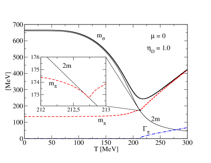
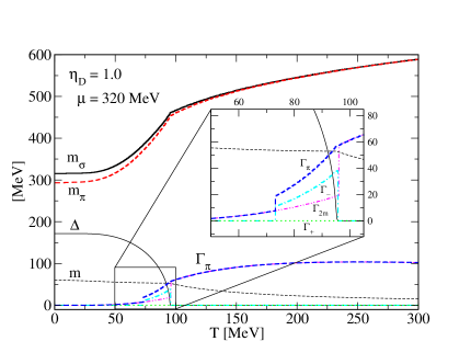
Figure 2: Left panel: Mass spectrum of mesons ($\pi$, $\sigma$) as a function of the temperature for vanishing chemical potential $\mu_{B}=0$ and strong diquark coupling $\eta_{D}=1.0$. The threshold $E_{\rm th}=2m_{q}$ for Mott dissociation of pions and occurrence of a nonvanishing decay width $\Gamma_{\pi}={\rm Im}~{}\Pi_{\pi}/m_{\pi}$ is reached at $T_{\rm Mott}=212.7$ MeV (see inset). Right panel: Mass spectrum of mesons ($\pi$, $\sigma$) as a function of the temperature for finite chemical potential $\mu_{B}=320$ MeV and strong diquark coupling $\eta_{D}=1.0$ in the 2SC phase. Below the threshold $E_{\rm th}=2~{}m_{q}$ for the onset of the decay width $\Gamma_{2m}$ there is another process due to the lower threshold $E_{+}-E_{-}$ switching on (see inset).

Next we want to discuss the pionic excitations in the presence of a diquark condensate in the 2SC phase, see the right panel of Fig. 2. We observe the remarkable fact that the 2SC condensate stabilizes the pion at $T=0$ as a true bound state, although the pion mass exceeds by far the threshold $2m$. This effect is due to a compensation of gapped and ungapped quark modes and has been discussed before by Ebert et al. Ebert:2004dr for $T=0$ only. Here we extend this study to the finite temperature case, where the pion obtains a finite width but is still a very good resonance.

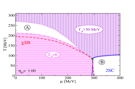
Figure 3: Phase diagram of two-flavor quark matter for the diquark coupling strength $\eta_{D}=1.0$. The pion is a stable bound state in the horizontally hatched region below the dash-dotted line which is correlated with critical line for chiral symmetry breaking (dashed). In the vertically hatched region above the dotted line the pion is a short-lived resonance with a width $\Gamma_{\pi}>50$ MeV ($\tau_{\pi}<1$ fm/c). There are two regions where the pion is a quasi-bound state in the quark plasma: (A) in the crossover region above the chiral phase transition and (B) in the color superconducting phase delimited by the solid line.

Finally, an interesting insight can come looking at Fig. 3. In this figure we have reported the essential phase diagram of the two-flavor quark matter in the case of coupling $\eta_{D}=1.00$. The dashed line represents the chiral crossover line and the solid line refers to the phase transition towards 2SC phase. The dot-dashed line shows the border above which the pion turns out to be a quasi bound state in the quark plasma. The dotted line indicates the region border (A) below which the quasi-stable pionic states have a lifetime greater than 1 fm/c, which is a typical lifetime of fireballs . Thus they would be measured as bound states and could be significant in the framework of HIC experiments. Region (B) confirms our claim about the absence of stable pions in a two-flavor superconductor. However this claim needs a comment. First of all, it can be easily understood how the presence of a finite diquark gap (2SC phase) at T=0 stabilizes the pion. Indeed as soon as the quark mass drops due to chiral symmetry restoration, the diquark gap tends to be finite and thus takes over the role of the quark mass in the dispersion relations. Roughly speaking the quark start to be dressed by his interactions. Thus the pion does not “feel” the drop of the quark mass. But as $\Delta$ melts with increasing $T$, the pion width $\Gamma_{\pi}$ raises, first slowly and then rapidly, reflecting the behaviour of $\Delta$ as a function of T. This leads inevitably to a destabilization of the the pion states in the vicinity of the 2SC phase border. The discussion of the mesonic modes in the 2SC phase points to a very rich spectrum of excitations which eventually leads to specific new observable signals of this hypothetical phase. The CBM experiment planned at FAIR Darmstadt and the NICA project at JINR Dubna could be capable of creating thermodynamical conditions for the observation of these excitations in the experiment. One promising signal could be the scalar resonance in the pion-pion scattering at the two-pion threshold which is in principle observable, e.g., in the two-photon decay channel Volkov:1997dx ; Blaschke:2006ss . However, the description of this state goes beyond the Gaussian approximation to which we restrict ourselves in this work.

3 Conclusions

In this work we have derived and evaluated the gap equations and the scalar-pseudoscalar meson spectra within a path integral approach to the two-flavor NJL type model of superconducting quark matter.

After fixing the parameters of the model to the light meson spectrum in the vacuum, the diquark coupling remains as a free parameter which has been used to extend the model beyond the traditional range of applications into the region of BEC-BCS crossover.

We have presented the phase diagram of quark matter at strong and very strong coupling. The origin of the BEC-BCS crossover in superconducting quark matter is the Mott transition for diquark bound states. We explain the physics of the Mott transition on the example of mesonic correlations. We have investigated the meson spectra (bound and scattering states) outside ($T>T_{c}$) and for the first time also inside ($T<T_{c}$) the color superconductivity region. We find the thresholds for the dissociation of pionic bound states into unbound, but resonant scattering states in the quark-antiquark continuum and we have shown that outside the $\chi$SB region where the pion is a zero-width bound state, there are two regions where it can be considered as a quasi-bound state with a lifetime exceeding that of a typical heavy-ion collision fireball: (A) the high-temperature $\chi$SB crossover region at low densities and (B) the high-density color superconducting phase at temperatures below 100 MeV.

References

- (1) B. Müller and J. L. Nagle, Ann. Rev. Nucl. Part. Sci., 56, 93 (2006)
- (2) E. Shuryak, Prog. Part. Nucl. Phys. , 53, 273 (2004)
- (3) E. V. Shuryak and I. Zahed, Phys. Rev. C, 70, 021901 (2004)
- (4) E. V. Shuryak, I. Zahed, Phys. Rev. D, 70, 054507 (2004)
- (5) D. A. Teaney, J. Phys. G, 30, S1247 (2004).
-
(6)
G. Policastro, D.T. Son and A.O. Starinets,
Phys. Rev. Lett. , 87, 081601 (2001);
P. Kovtun, D.T. Son and A.O. Starinets, JHEP, 0310, 064 (2003). - (7) D. B. Blaschke and K. A. Bugaev, Fizika B, 13, 491 (2004) [arXiv:nucl-th/0311021].
- (8) D. Blaschke, AIP Conf. Proc. , 775, 151 (2005).
- (9) H. Abuki, Nucl. Phys. A, 791, 117 (2007)
- (10) E. V. Shuryak, arXiv:nucl-th/0606046
- (11) N. Mott, Rev. Mod. Phys., 40, 677 (1968)
- (12) Pairing in fermionic system, edited by A. Sedrakian, J. W. Clark, M. Alford, World Scientific, Singapore, 2006
- (13) F. X. Bronold,H. Fehske, Phys. Rev. B, 74, 165107 (2006)
- (14) R. Redmer, B. Holst, H. Juranek, N. Nettelmann, V. Schwarz, J. Phys. A, 39, 4479 (2006)
- (15) M. Schmidt, G. Röpke, H. Schulz, Ann. Phys., 202, 57 (1990)
- (16) H. Stein, A. Schnell, T. Alm, G. Röpke, Z. Phys. A, 351, 295 (1995)
- (17) A. Schnell, G. Röpke, P. Schuck, Phys. Rev. Lett., 83, 1926 (1999)
- (18) M. Kitazawa, T. Koide, T. Kunihiro, Y. Nemoto, Phys. Rev. D, 65, 091504 (2002)
- (19) M. Kitazawa, T. Koide, T. Kunihiro, Y. Nemoto, Phys. Rev. D, 70, 056003 (2004)
- (20) D. Blaschke, D. Ebert, K. G. Klimenko, M. K. Volkov, V. L. Yudichev, Phys. Rev. D, 70, 014006 (2004)
- (21) D. Blaschke, S. Fredriksson, H. Grigorian, A. M. Öztas, F. Sandin, Phys. Rev. D, 72, 065020 (2005)
- (22) Q. Chen, J. Stajic, K. Levin, J. Low Temp. Phys, 32, 406 (2005)
- (23) E. Calzetta, B. L. Hu and A. M. Rey, Phys. Rev. A, 73, 023610 (2006)
- (24) V. Gurarie and L. Radzihovsky, Ann. Phys, 322, 2 (2007)
- (25) M: Greiner, C. A: Regal and D. S. Jin, Nature, 426, 537 (2003)
- (26) M. W. Zwierlein, C. A. Stan, C. H. Schunck, S. M. Raupach, S. Gupta, Z. Hadzibabic and W. Ketterle, Phys. Rev. Lett., 91, 250401 (2003)
- (27) M. W. Zwierlein, J. R. Abo-Shaeer, A. Schirotzek, C. H. Schunck and W. Ketterle, Nature, 435, 1047 (2003)
- (28) M. Greiner, O. Mandel, T. Rom, A. Altmeyer, A. Widera, T. W. Hänsch and I. Bloch, Physica B, 329, 11 (2003)
- (29) J. Deng, A. Schmitt, Q. Wang, Phys. Rev. D, 76, 034013 (2007)
- (30) G. Sun, L. He, P. Zhuang, Phys. Rev. D, 75, 096004 (2007)
- (31) Finite-temperature Field Theory, edited by J. Kapusta, Cambridge University Press, Cambridge, 1989, p.26.
- (32) M. Buballa, Phys. Rept., 407, 205 (2005)
- (33) H. Grigorian, Phys. Part. Nucl. Lett., 4, 223 (2007)
- (34) H. Kleinert, Fortsch. Phys., 26, 565 (1978)
- (35) D. Ebert, K. K. Klimenko, V. L. Yudichev, Phys. Rev. C, 72, 015201 (2005)
- (36) R. Anglani, D. Blaschke, D. Zablocki, in preparation.
- (37) J. Hüfner, S. P. Klevansky, P. Rehberg, Nucl. Phys. A, 606, 260 (1996)
- (38) V. Gurarie, L. Radzihovsky, Ann. Phys., 322, 2 (2007)
- (39) M. K. Volkov, E. A. Kuraev, D. Blaschke, G. Ropke and S. M. Schmidt, Phys. Lett. B, 424, 235 (1998)
- (40) D. Blaschke, Yu. L. Kalinovsky, A. E. Radzhabov and M. K. Volkov, Phys. Part. Nucl. Lett., 3, 327 (2006)