Perturbation Theory Reloaded II: Non-linear Bias, Baryon Acoustic Oscillations and Millennium Simulation In Real Space

Abstract

We calculate the non-linear galaxy power spectrum in real space, including non-linear distortion of the Baryon Acoustic Oscillations, using the standard 3rd-order perturbation theory (PT). The calculation is based upon the assumption that the number density of galaxies is a local function of the underlying, non-linear density field. The galaxy bias is allowed to be both non-linear and stochastic. We show that the PT calculation agrees with the galaxy power spectrum estimated from the Millennium Simulation, in the weakly non-linear regime (defined by the matter power spectrum) at high redshifts, $1\leq z\leq 6$. We also show that, once 3 free parameters characterizing galaxy bias are marginalized over, the PT power spectrum fit to the Millennium Simulation data yields unbiased estimates of the distance scale, $D$, to within the statistical error. This distance scale corresponds to the angular diameter distance, $D_{A}(z)$, and the expansion rate, $H(z)$, in real galaxy surveys. Our results presented in this paper are still restricted to real space. The future work should include the effects of non-linear redshift space distortion. Nevertheless, our results indicate that non-linear galaxy bias in the weakly non-linear regime at high redshifts is reasonably under control.

1. Introduction

Surveys of galaxies are the oldest way of mapping cosmological fluctuations. Over the last three decades they have been used for measuring cosmological parameters, such as the matter density of the universe, $\Omega_{m}$ (see Peebles, 1993, for a review).

The galaxy surveys are largely complementary to CMB, as they allow us to determine the important cosmological parameters that remain poorly constrained by the CMB data alone (e.g., Takada et al., 2006): e.g., the mass of neutrinos, the shape of the primordial power spectrum, and the properties of dark energy.

The latest data sets, Two Degree Field Galaxy Redshift Survey (2dFGRS, Cole et al., 2005) and Sloan Digital Sky Survey (SDSS, Tegmark et al., 2006), have enabled us to determine most of the cosmological parameters to better than 5% accuracy, when combined with the Cosmic Microwave Background (CMB) data from the Wilkinson Microwave Anisotropy Probe (Bennett et al., 2003; Spergel et al., 2003, 2007; Hinshaw et al., 2008; Dunkley et al., 2008; Komatsu et al., 2008).

The galaxy power spectrum, the Fourier transform of the galaxy two point correlation function, has been used widely for extracting cosmological information from the galaxy survey data. The amplitude, overall shape, as well as oscillatory features (called the Baryon Acoustic Oscillations, or BAOs) contain a wealth of cosmological information (see Weinberg, 2008, for a recent review). In order to extract this information correctly, we must understand how the observed galaxy power spectra are related to the underlying cosmological models.

How do we model the galaxy power spectrum? We may use the cosmological perturbation theory (PT). The accuracy of the linear PT has been verified observationally by the temperature and polarization data of CMB measured by WMAP (Hinshaw et al., 2003, 2007; Kogut et al., 2003; Page et al., 2007; Nolta et al., 2008). However, we cannot use the linear PT for the galaxy power spectrum, as the matter density field grows non-linearly due to gravitational instability. One must therefore use the non-linear PT.

There are three sources of non-linearities:

• Non-linear evolution of the underlying matter density field, which alters the matter power spectrum away from the linear prediction.

• Non-linear galaxy bias, or non-linear mapping between the underlying matter density field and the distribution of collapsed objects such as dark matter halos and galaxies, which alters the galaxy power spectrum away from the matter power spectrum.

• Non-linear redshift space distortion, which arises as the observed redshifts of galaxies used for measuring locations of galaxies along the line of sight contain both the Hubble expansion and the peculiar velocity of galaxies. This leads to the systematic shifts in the line-of-sight positions of galaxies, altering the galaxy power spectrum in redshift space away from that in real space.

Using the 3rd-order PT (see Bernardeau et al., 2002, for a review) we have shown that the first effect can be modeled accurately in the weakly non-linear regime (Jeong & Komatsu, 2006, hereafter Paper I). In this paper we address the second effect, the non-linear galaxy bias, using the 3rd-order PT. We will address the third effect, the non-linear redshift space distortion, in the future work.

Our study is motivated by recently proposed high redshift galaxy surveys such as Cosmic Inflation Probe (CIP), Hobby-Eberly Dark Energy Experiment (HETDEX; Hill et al., 2004), Baryon Oscillation Spectroscopic Survey (BOSS), and Wide-field Fiber-fed Multi Object Spectrograph survey (WFMOS; Glazebrook et al., 2005), to mention a few. These proposed surveys will observe the galaxy power spectra to the unprecedented precision, which demands the precision modeling of the galaxy power spectrum at 1% accuracy or better.

Over the last decade, the non-linear PT, including modeling of non-linear galaxy power spectra, had been studied actively (see Bernardeau et al., 2002, for a review). However, PT had never been applied to the real data such as 2dFGRS or SDSS, as non-linearities are too strong for PT to be valid at low redshifts, $z<1$ (e.g., Meiksin et al., 1999). At high redshifts, i.e., $z>1$, however, PT is expected to perform better because of weaker non-linearity. In Paper I we have shown that the matter power spectrum computed from the 3rd-order PT describes that from $N$-body simulations accurately.

But, what about the galaxy power spectrum? One may generally expect that, since non-linearities were milder in a high-$z$ universe, there should be a plenty of room for PT to be a good approximation. On the other hand, galaxies were more highly biased at higher redshifts for a given mass, and therefore one might suspect, somewhat naively, that non-linear bias could compromise the success of PT. In this paper we shall show that is not the case, and PT does provide a good approximation to the galaxy power spectrum at high redshifts.

This paper is organized as follows. In § 2 we give the formula for the 3rd-order PT galaxy power spectrum. In § 3 we compare the 3rd-order PT matter power spectrum with the matter power spectrum estimated from the Millennium Simulation (Springel et al., 2005), in order to confirm our previous results (Paper I) with the Millennium Simulation. In § 4 we show that the PT calculation of the galaxy power spectrum agrees with the galaxy power spectrum estimated from the Millennium Simulation in the weakly non-linear regime (defined by the matter power spectrum) at high redshifts, $1\leq z\leq 6$. In § 5 we extract the distance scale from the Millennium Simulation, which is related to the angular diameter distance and the expansion rate of the universe in real surveys. In § 6 we give discussion and conclusions.

2. Non-linear galaxy power spectrum from perturbation theory

2.1. Locality Assumption

Galaxies are biased tracers of the underlying density field (Kaiser, 1984), which implies that the distribution of galaxies depends on the underlying matter density fluctuations in a complex way. This relation must depend upon the detailed galaxy formation processes, which are not yet understood completely.

However, on large enough scales, one may approximate this function as a local function of the underlying density fluctuations, i.e., the number density of galaxies at a given position in the universe is given solely by the underlying matter density at the same position. With this approximation, one may expand the density fluctuations of galaxies, $\delta_{g}$, in terms of the underlying matter density fluctuations, as (Fry & Gaztanaga, 1993; McDonald, 2006)

$$\delta_{g}(\mathbf{x})=\epsilon+b_{1}\delta(\mathbf{x})+\frac{1}{2}b_{2}\delta^{2}(\mathbf{x})+\frac{1}{6}b_{3}\delta^{3}(\mathbf{x})+\dots,$$ (1)

where $b_{n}$ are the galaxy bias parameters, and $\epsilon$ is a random variable that represents the “stochasticity” of the galaxy bias, i.e., the relation between $\delta_{g}(\mathbf{x})$ and $\delta(\mathbf{x})$ is not deterministic, but contains some noise (e.g., Yoshikawa et al., 2001, and references therein). We assume that the stochasticity is white noise, and is uncorrelated with the density fluctuations, i.e., $\langle\epsilon\delta\rangle=0$. While both of these assumptions should be violated at some small scales, we assume that these are valid assumptions on the scales that we are interested in – namely, on the scales where the 3rd-order PT describes the non-linear matter power spectrum with 1% accuracy. Since both bias parameters and stochasticity evolve in time (Fry, 1996; Tegmark & Peebles, 1998), we allow them to depend on redshifts.

One obtains the traditional “linear bias model” when the Taylor series expansion given in Eq. (1) is truncated at the first order and the stochasticity is ignored.

The precise values of the galaxy bias parameters depend on the galaxy formation processes, and different types of galaxies have different galaxy bias parameters. However, we are not interested in the precise values of the galaxy bias parameters, but only interested in extracting cosmological parameters from the observed galaxy power spectra with all the bias parameters marginalized over.

2.2. 3rd-order PT galaxy power spectrum

The analysis in this paper adopts the framework of McDonald (2006), and we briefly summarize the result for clarity. We shall use the 3rd-order PT; thus, we shall keep the terms up to the 3rd order in $\delta$. The resulting power spectrum can be written in terms of the linear matter power spectrum, $P_{L}(k)$, and the 3rd order matter power spectrum, $P_{\delta\delta}(k)$, as

$$P_{g}(k)=P_{0}+\tilde{b}_{1}^{2}\biggl{[}P_{\delta\delta}(k)+\tilde{b}_{2}P_{b2}(k)+\tilde{b}_{2}^{2}P_{b22}(k)\biggl{]},$$ (2)

where $P_{b2}$ and $P_{b22}$ are given by

$$P_{b2}=2\int\frac{d^{3}\mathbf{q}}{(2\pi)^{3}}P_{L}(q)P_{L}(|\mathbf{k}-\mathbf{q}|)F_{2}^{(s)}(\mathbf{q},\mathbf{k}-\mathbf{q}),$$

and

$$P_{b22}=\frac{1}{2}\int\frac{d^{3}\mathbf{q}}{(2\pi)^{3}}P_{L}(q)\biggl{[}P_{L}(|\mathbf{k}-\mathbf{q}|)-P(q)\biggl{]},$$

respectively, with $F_{2}^{(2)}$ given by

$$F_{2}^{(s)}(\mathbf{q}_{1},\mathbf{q}_{2})=\frac{5}{7}+\frac{2}{7}\frac{(\mathbf{q}_{1}\cdot\mathbf{q}_{2})^{2}}{q_{1}^{2}q_{2}^{2}}+\frac{\mathbf{q}_{2}\cdot\mathbf{q}_{2}}{2}\left(\frac{1}{q_{1}^{2}}+\frac{1}{q_{2}^{2}}\right).$$

We use the standard formula for $P_{\delta\delta}$ (see Eq. (14) of Paper I and references therein). Here, $\tilde{b}_{1}$, $\tilde{b}_{2}$, and $P_{0}$ are the non-linear bias parameters, which are given in terms of the original coefficients for the Taylor expansion as

$$\tilde{b}_{1}^{2} = b_{1}^{2}+b_{1}b_{3}\sigma^{2}+\frac{68}{21}b_{1}b_{2}\sigma^{2},$$

$$\tilde{b}_{2} = \frac{b_{2}}{\tilde{b}_{1}},$$ (3)

$$P_{0} = \langle\epsilon^{2}\rangle+\frac{1}{2}b_{2}^{2}\int\frac{k^{2}dk}{2\pi^{2}}P_{L}^{2}(k),$$

where $\sigma$ is the r.m.s. of density fluctuations.

We will never have to deal with the original coefficients, $b_{1}$, $b_{2}$, $b_{3}$, or $\epsilon$. Instead, we will only use the re-parametrized bias parameters, $\tilde{b}_{1}$, $\tilde{b}_{2}$, and $P_{0}$, as these are related more directly to the observables. As shown by McDonald (2006), in the large-scale limit, $k\rightarrow 0$, one finds

$$P_{g}(k)\rightarrow P_{0}+\tilde{b}_{1}^{2}P_{L}(k).$$ (4)

Therefore, in the large-scale limit one recovers the traditional linear bias model plus the constant term. Note that $\tilde{b}_{1}$ is the same as what is called the “effective bias” in Heavens et al. (1998).

Throughout this paper we shall use Eq. (2) for calculating the non-linear galaxy power spectra.

2.3. Why we do not care about the precise values of bias parameters

The precise values of the galaxy bias parameters depend on the details of the galaxy formation and evolution, as well as on galaxy types, luminosities, and so on.

However, our goal is to extract the cosmological information from the observed galaxy power spectra, without having to worry about which galaxies we are using as tracers of the underlying density field.

Therefore, we will marginalize the likelihood function over the bias parameters, without ever paying attention to their precise values. Is this approach sensible?

One might hope that one should be able to calculate the bias parameters for given properties of galaxies from the first principles using, e.g., sophisticated numerical simulations.

Less numerically expensive way of doing the same thing would be to use the semi-analytical halo model approach, calibrated with a smaller set of numerical simulations (see Cooray & Sheth, 2002, for a review). Using the peak-background split method (Sheth & Tormen, 1999) based upon the excursion set approach (Bond et al., 1991), one can calculate $b_{1}$, $b_{2}$, $b_{3}$, etc., the coefficients of the Taylor series expansion given in Eq. (1), for the density of dark matter halos. Once the bias parameters for dark matter halos are specified, the galaxy bias parameters may be calculated using the so-called Halo Occupation Distribution (HOD) (Seljak, 2000).

Smith et al. (2007) have attempted this approach, and shown that it is difficult to calculate even the power spectrum of dark matter halos that matches $N$-body simulations. The halo-model predictions for bias parameters are not yet accurate enough, and we do not yet have a correct model for $P_{0}$.

The situation would be even worse for the galaxy power spectrum, as we would have to model the HOD in addition to the halo bias. At the moment the form of HOD is basically a free empirical function. We therefore feel that it is dangerous to rely on our limited understanding of these complications for computing the bias parameters.

This is the reason why we have decided to give up predicting the precise values of bias parameters entirely. Instead, we shall treat 3 bias parameters, $\tilde{b}_{1}$, $\tilde{b}_{2}$, and $P_{0}$, as free parameters, and fit them to the observed galaxy power spectra simultaneously with the cosmological parameters.

The most important question that we must ask is the following, “using the 3rd-order PT with 3 bias parameters, can we extract the correct cosmological parameters from the galaxy power spectra?” If the answer is yes, we will not have to worry about the precise values of bias parameters anymore.

3. Dark Matter Power spectrum from Millennium Simulation

In this section we show that the matter power spectrum computed from the 3rd-order PT agrees with that estimated from the Millennium Simulation (Springel et al., 2005). This result confirms our previous finding (Paper I).

Using the result obtained in this section we define the maximum wavenumber, $k_{max}$, below which the 3rd-order PT may be trusted. The matter power spectrum gives an unambiguous definition of $k_{max}$, which will then be used thereafter when we analyze power spectra of halos and galaxies in § 4.

3.1. Millennium Simulation

The Millennium simulation (Springel et al., 2005) is a large $N$-body simulation with the box size of $(500~{}\textrm{Mpc}/h)^{3}$ and $2160^{3}$ dark matter particles. The cosmological parameters used in the simulation are $(\Omega_{dm},\Omega_{b},\Omega_{\Lambda},h)=(0.205,~{}0.045,~{}0.75,~{}0.73)$.

The primordial power spectrum used in the simulation is the scale-invariant Peebles-Harrison-Zel’dovich spectrum, $n_{s}=1.0$, and the linear r.m.s. density fluctuation smoothed with a top-hat filter of radius $8~{}h^{-1}\mathrm{Mpc}$ is $\sigma_{8}=0.9$. Note that these values are significantly larger than the latest values found from the WMAP 5-year data, $\sigma_{8}\simeq 0.8$ and $n_{s}\simeq 0.96$ (Dunkley et al., 2008; Komatsu et al., 2008), which implies that non-linearities in the Millennium Simulation should be stronger than those in our Universe.

The Millennium Simulation was carried out using the GADGET code (Springel et al., 2001; Springel, 2005). The GADGET uses the tree Particle Mesh (tree-PM) gravity solver, which tends to have a larger dynamic range than the traditional PM solver for the same box size and the same number of particles (and meshes)(Heitmann et al., 2007). Therefore, the matter power spectrum from the Millennium Simulation does not suffer from an artificial suppression of power as much as those from the PM codes.

The initial particle distribution was generated at the initial redshift of $z_{ini}=127$ using the standard Zel’dovich approximation. While the initial conditions generated from the standard Zel’dovich approximation tend to produce an artificial suppression of power at later times, and the higher-order scheme such as the second-order Lagrangian perturbation theory usually produces better results (Scoccimarro, 1998; Crocce et al., 2006), the initial redshift of the Millennium Simulation, $z_{ini}=127$, is reasonably high for the resulting power spectra to have converged in the weakly non-linear regime.

The mass of each dark matter particle in the simulation is $M_{dm}=8.6\times 10^{8}M_{\odot}/h$. They require at least 20 particles per halo for their halo finder, and thus the minimum mass resolution of halos is given by $M_{halo}\geq 20M_{dm}\simeq 1.7\times 10^{10}~{}M_{\odot}/h$. Therefore, the Millennium Simulation covers the mass range that is relevant to real galaxy surveys that would detect galaxies with masses in the range of $M\simeq 10^{11}-10^{12}~{}M_{\odot}$. This property distinguishes our study from the previous studies on non-linear distortion of BAOs due to galaxy bias (e.g., Smith et al., 2007; Huff et al., 2007), whose mass resolution was greater than $\sim 10^{12}~{}M_{\odot}$.

In addition to the dark matter halos, the Millennium database also provides galaxy catalogues from two different semi-analytic galaxy formation models (De Lucia & Blaizot, 2007; Croton et al., 2006; Bower et al., 2006; Benson et al., 2003; Cole et al., 2000). These catalogues give us an excellent opportunity for testing validity of the non-linear galaxy power spectrum model based upon the 3rd-order PT with the unprecedented precision.

3.2. 3rd-order PT versus Millennium Simulation: Dark Matter Power Spectrum

First, we compare the matter power spectrum from the Millennium simulation with the 3rd-order PT calculation. The matter power spectrum we use here was measured directly from the Millennium simulation on the fly.

Figure 1.— Matter power spectrum at $z=0$, 1, 2, 3, 4, 5 and 6 (from top to bottom) derived from the Millennium Simulation (dashed lines), the 3rd-order PT (solid lines), and the linear PT (dot-dashed lines).

Figure 2.— Dimensionless matter power spectrum, $\Delta^{2}(k)$, at $z=1$, 2, 3, 4, 5, and 6. The dashed and solid lines show the Millennium Simulation data and the 3rd-order PT calculation, respectively. The dot-dashed lines show the linear power spectrum.

Figure 3.— Fractional difference between the matter power spectra from the 3rd-order PT and that from the Millennium Simulation, $P_{m}^{sim}(k)/P_{m}^{PT}-1$ (dots with errorbars). The solid lines show the perfect match, while the dashed lines show $\pm 2\%$ accuracy. We also show $k_{max}(z)$, below which we trust the prediction from the 3rd-order PT, as a vertical dotted line.

Table 1Maximum wavenumbers, $k_{max}$, for the Millennium Simulation

$z$	$k_{max}$	$\tilde{k}_{max}$
	($h/\mathrm{Mpc}$)	$(h/\mathrm{Mpc})$
6	1.5	1.99
5	1.3	1.37
4	1.2	1.02
3	1.0	0.60
2	0.25	0.35
1	0.15	0.20

Note. — $z$: redshift

$k_{max}$: the maximum wavenumber for the simulated $P_{m}(k)$ to agree with the PT calculation at 2% accuracy within the statistical error of the Millennium Simulation

$\tilde{k}_{max}$: $\tilde{k}_{max}$ is defined by $\Delta^{2}_{m}(\tilde{k}_{max})=0.4$ which is the criteria recommended in Paper I.

Figure 4.— Distortion of BAOs due to non-linear matter clustering. All of the power spectra have been divided by a smooth power spectrum without baryonic oscillations from eq. (29) of Eisenstein & Hu (1998). The error bars show the simulation data, while the solid lines show the PT calculations. The dot-dashed lines show the linear theory calculations. The power spectrum data shown here have been taken from Figure 6 of Springel et al. (2005).

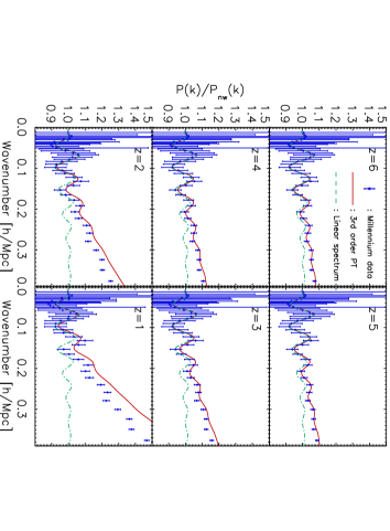
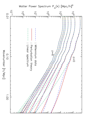
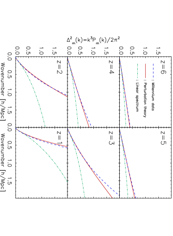
Figure 1 shows the matter power spectrum from the Millennium simulation (dashed lines), the 3rd-order PT calculation (solid lines), and the linear PT (dot-dashed lines) for seven different redshifts, $z=0$, 1, 2, 3, 4, 5, and 6. The analytical calculation of the 3rd-order PT reproduces the non-linear matter power spectrum from the Millennium Simulation accurately at high redshifts, i.e., $z>1$, up to certain maximum wavenumbers, $k_{max}$, that will be specified below. To facilitate the comparison better, we show the dimensionless matter power spectrum, $\Delta_{m}^{2}(k)\equiv k^{3}P_{m}(k)/2\pi^{2}$, in Figure 2.

We find the maximum wavenumber, $k_{max}(z)$, below which we trust the prediction from the 3rd-order PT, by comparing the matter power spectrum from PT and the Millennium Simulation. The values of $k_{max}$ found here will be used later when we analyze the halo/galaxy power spectra.

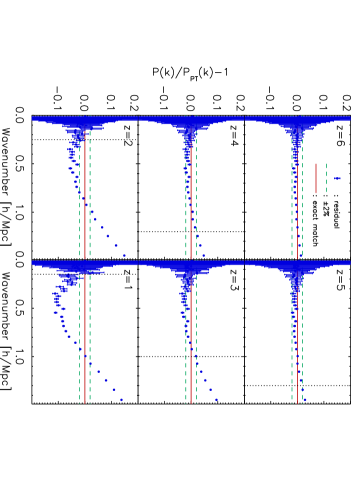
In Paper I we have defined $k_{max}$ such that the fractional difference between PT and the average of $\sim 100$ simulations is 1%. Here, we have only one realization, and thus the results are subject to statistical fluctuations that might be peculiar to this particular realization. Therefore, we relax our criteria for $k_{max}$: we define $k_{max}$ such that the fractional difference between PT and the Millennium Simulation is 2%.

Figure 3 shows the fractional differences at $z=1$, 2, 3, 4, 5, and 6. Since we have only one realization, we cannot compute statistical errors from the standard deviation of multiple realizations. Therefore, we derive errors from the leading-order 4-point function assuming Gaussianity of the underlying density fluctuations (see Appendix A), $\sigma_{P(k)}=P(k)/\sqrt{N_{k}}$, where $N_{k}$ is the number of independent Fourier modes per bin at a given $k$ shown in Figure 3.

We give the values of $k_{max}$ in Table 1. We shall use these values when we fit the halo/galaxy power spectrum in the next section. Note that $k_{max}$ decreases rapidly below $z=2$. It is because $P(k)/P_{PT}(k)-1$ is not a monotonic function of $k$. The dip in $P(k)/P_{PT}(k)-1$ is larger than $2\%$ at lower redshift, $z<2$, while it is inside of the $2\%$ range at $z\geq 3$. Therefore, our criteria of $2\%$ make that sudden change. This feature is due to the limitation of the standard 3rd order PT. However, we can remove this feature by using the improved perturbation theory, e.g. using renormalization group techniques. (See, Figure 9 of Matarrese & Pietroni (2007).)

We also give the values of $\tilde{k}_{max}$, for which $\Delta^{2}_{m}(\tilde{k}_{max})=0.4$ (criteria recommended in Paper I). The difference between $k_{max}$ and $\tilde{k}_{max}$ is probably due to the fact that we have only one realization of the Millennium Simulation, and thus estimation of $k_{max}$ is noisier. Note that the values of $\tilde{k}_{max}$ given in Table 1 are smaller than those given in Paper I. This is simply because $\sigma_{8}$ of the Millennium Simulation ($\sigma_{8}=0.9$) is larger than that of Paper I ($\sigma_{8}=0.8$).

In Figure 4 we show the matter power spectra divided a smooth spectra without BAOs (Eq. (29) of Eisenstein & Hu, 1998). The results are consistent with what we have found in Paper I: although BAOs in the matter power spectrum are distorted heavily by non-linear evolution of matter fluctuations, the analytical predictions from the 3rd-order PT capture the distortions very well at high redshifts, $z>2$.

At lower redshifts, $z\sim 1$, the 3rd-order PT is clearly insufficient, and one needs to go beyond the standard PT. This is a subject of recent studies (Crocce & Scoccimarro, 2008; Matarrese & Pietroni, 2007; Taruya & Hiramatsu, 2008; Valageas, 2007; Matsubara, 2008; McDonald, 2007).

4. HALO/GALAXY POWER SPECTRUM AND THE NON-LINEAR BIAS MODEL

In this section we compare the 3rd-order PT galaxy power spectrum with the power spectra of dark matter halos and galaxies estimated from the Millennium Simulation. After briefly describing the analysis method in § 4.1, we analyze the halo bias and galaxy bias in § 4.2 and § 4.3, respectively. We then study the dependence of bias parameters on halo/galaxy mass in § 4.4.

4.1. Analysis method

Table 2Summary of six snapshots from the Millennium Simulation

$z$	$z_{\mathrm{show}}$	$N_{h}$	$1/n_{h}$	$N_{Mg}$	$1/n_{Mg}$	$N_{Dg}$	$1/n_{Dg}$
			($[\mathrm{Mpc}/h]^{3}$)		($[\mathrm{Mpc}/h]^{3}$)		($[\mathrm{Mpc}/h]^{3}$)
5.724	6	5,741,720	21.770	6,267,471	19.944	4,562,368	27.398
4.888	5	8,599,981	14.535	9,724,669	12.854	7,604,063	16.439
4.179	4	11,338,698	11.024	13,272,933	9.418	10,960,404	11.405
3.060	3	15,449,221	8.091	19,325,842	6.468	17,238,935	7.251
2.070	2	17,930,143	6.972	23,885,840	5.233	22,962,129	5.444
1.078	1	18,580,497	6.727	26,359,329	4.742	27,615,058	4.527

Note. — $z$: the exact redshift of each snapshot

$z_{\mathrm{show}}$: the redshift we quote in this paper

$N_{h}$: the number of MPA halos in each snapshot; $1/n_{h}$: the corresponding Poisson shot noise

$N_{Mg}$: the number of MPA galaxies in each snapshot; $1/n_{Mg}$: the corresponding Poisson shot noise

$N_{Dg}$: the number of Durham galaxies in each snapshot; $1/n_{Dg}$: the corresponding Poisson shot noise

We choose six redshifts between $1\leq z\leq 6$ from 63 snapshots of the Millennium Simulation, and use all the available catalog of halos (MPA Halo (MHalo), hereafter ‘halo’) and two galaxy catalogues (MPA Galaxies, hereafter ‘Mgalaxy’; Durham Galaxies, hereafter ‘Dgalaxy’) at each redshift. The exact values of redshifts and the other relevant information of chosen snapshots are summarized in Table 2.

Halos are the groups of matter particles found directly from the Millennium Simulation. First, the dark matter groups (called FOF group) are identified by using Friends-of-Friends (FoF) algorithm with a linking length equal to 0.2 of the mean particle separation. Then, each FoF group is divided into the gravitationally bound local overdense regions, which we call halos here.

Mgalaxies and Dgalaxies are the galaxies assigned to the halos using two different semi-analytic galaxy formation codes: L-Galaxies (Mgalaxies, De Lucia & Blaizot, 2007; Croton et al., 2006) and GALFORM (Dgalaxies, Bower et al., 2006; Benson et al., 2003; Cole et al., 2000).

While both models successfully explain a number of observational properties of galaxies like the break shape of the galaxy luminosity function, star formation rate, etc, they differ in detailed implementation. For example, while the L-Galaxies code uses the halo merger tree constructed by MHalos, the GALFORM code uses different criteria for identifying subhalos inside the FOF group, and thus uses a different merger tree. Also, two models use different gas cooling prescriptions and different initial mass functions (IMF) of star formation: L-Galaxies and GALFORM define the cooling radius, within which gas has a sufficient time to cool, by comparing the cooling time with halo dynamical time and the age of the halo, respectively. Cold gas turns into stars with two different IMFs: the L-Galaxies code ueses IMF from Chabrier (2003) and the GALFORM code uses Kennicutt (1983). In addition to that, they treat AGN (Active Galactic Nucleus) feedback differently: the L-Galaxies code introduces a parametric model of AGN feedback depending on the black hole mass and the virial velocity of halo, and the GALFORM code imposes the condition that cooling flow is quenched when the energy released by radiative cooling (cooling luminosity) is less than some fraction (which is modeled by a parameter, $\epsilon_{\mathrm{SMBH}}$) of Eddington luminosity of the black hole. For more detailed comparison of the two model, we refer readers to the original papers cited above.

We compute the halo/galaxy power spectra from the Millennium Simulation as follows:

• Use the Cloud-In-Cell (CIC) mass distribution scheme to calculate the density field on $1024^{3}$ regular grid points from each catalog.

• Fourier-transform the discretized density field using FFTW.

• Deconvolve the effect of the CIC pixelization and aliasing effect. We divide $P(\mathbf{k},z)\equiv|\delta(\mathbf{k},z)|^{2}$ at each cell by the following window function (Jing, 2005):

  $$W(\mathbf{k})=\prod_{i=1}^{3}\left[1-\frac{2}{3}\sin^{2}\left(\frac{\pi k_{i}}{2k_{N}}\right)\right],$$ (5)

  where $\mathbf{k}=(k_{1},k_{2},k_{3})$, and $k_{N}\equiv\pi/H$ is the Nyquist frequency, ($H$ is the physical size of the grid).

• Compute $P(k,z)$ by taking the angular average of CIC-corrected $P(\mathbf{k},z)\equiv|\delta(\mathbf{k},z)|^{2}$ within a spherical shell defined by $k-\Delta k/2<|\mathbf{k}|<k+\Delta k/2$. Here, $\Delta k=2\pi/500~{}[h/\rm{Mpc}]$ is the fundamental frequency that corresponds to the box size of the Millennium Simulation.

From the measured power spectra we find the maximum likelihood values of the bias parameters using the likelihood function approximated as a Gaussian:

$$\mathcal{L}(\tilde{b}_{1},\tilde{b}_{2},P_{0})=\prod_{k_{i}<k_{max}}\frac{1}{\sqrt{2\pi\sigma_{Pi}^{2}}}\exp\left[-\frac{(P_{obs,i}-P_{g,i})^{2}}{2\sigma_{Pi}^{2}}\right],$$ (6)

where $k_{i}$’s are integer multiples of the fundamental frequency $\Delta k$, $P_{obs,i}$ is the measured power spectrum at $k=k_{i}$, $P_{g,i}$ is the theoretical model given by Eq. (2), and $\sigma_{Pi}$ is the statistical error in the measured power spectrum.

We estimate $\sigma_{Pi}$ in the same way as in § 3 (see also Appendix A). However, the power spectrum of the point-like particles like halos and galaxies includes the Poisson shot noise, $1/n$, where $n$ is the number density of objects, on top of the power spectrum due to clustering. Therefore, $\sigma_{Pi}$ must also include the shot-noise contribution. We use

$$\sigma_{Pi}=\sigma_{P}(k_{i})=\sqrt{\frac{1}{N_{ki}}}\left[P_{g}(k_{i})+\frac{1}{n}\right],$$ (7)

where

$$N_{ki}=2\pi\left(\frac{k}{\Delta k}\right)^{2}$$ (8)

is the number of independent Fourier modes used for estimating the power spectrum and $P_{g}(k_{i})$ is the halo/galaxy power spectrum at $k=k_{i}$. Here, $\Delta k=2\pi/(500~{}h^{-1}~{}\rm{Mpc})$ is the fundamental wavenumber of the Millennium Simulation. Note that we subtract the Poisson shot noise contribution, $P_{shot}=1/n$, from the observed power spectrum before the likelihood analysis.

Eq. (7) shows that the error on $P_{obs}(k)$ depends upon the underlying $P_{g}(k)$. For the actual data analysis one should vary $P_{g}(k)$ in the numerator of Eq. (6) as well as that in $\sigma_{Pi}$, simultaneously. However, to simplify the analysis, we evaluate the likelihood function in an iterative way: we first find the best-fitting $P_{g}(k)$ using $\sigma_{Pi}$ with $P_{g}(k)$ in Eq. (7) replaced by $P_{obs}(k)$. Let us call this $\tilde{P}_{g}(k)$. We then use $\tilde{P}_{g}(k)$ in Eq. (7) for finding the best-fitting $P_{g}(k)$ that we shall report in this paper. Note that we iterate this procedure only once for current study.

Finally, we compute the 1-d marginalized 1-$\sigma$ interval (or the marginalized $68.27\%$ confidence interval) of each bias parameter by integrating the likelihood function (Eq. (6)), assuming a flat prior on the bias parameters (see also Appendix B).

We first analyze the power spectrum of halos (in § 4.2) as well as that of galaxies (in § 4.3) using all the halos and all the galaxies in the Millennium halo/galaxy catalogues. We then study the mass dependence of bias parameters in § 4.4.

In order to show that the non-linear bias model (Eq. 2) provides a much better fit than the linear bias model, we also fit the measured power spectra with two linear bias models: (i) linear bias with the linear matter power spectrum, and (ii) linear bias with the non-linear matter power spectrum from the 3rd-order PT. When fitting with the linear model, we use $k_{max}=0.15~{}[h/\mathrm{Mpc}]$ for all redshift bins.

4.2. Halo power spectra

4.2.1 Measuring non-linear halo bias parameters

Figure 5.— Halo power spectra from the Millennium Simulation at $z=1$, 2, 3, 4, 5, and 6. Also shown in smaller panels are the residual of fits. The points with errorbars show the measured halo power spectra, while the solid, dashed, and dot-dashed lines show the best-fitting non-linear bias model (Eq. (2)), the best-fitting linear bias with the non-linear matter power spectrum, and the best-fitting linear bias with the linear matter power spectrum, respectively. Both linear models have been fit for $k_{max,linear}=0.15~{}[h~{}\mathrm{Mpc}^{-1}]$, whereas $k_{max}(z)$ given in Table 1 (also marked in each panel) have been used for the non-linear bias model.

Table 3Non-linear halo bias parameters and the corresponding 68% interval estimated from the MPA halo power spectra

$z$	$\tilde{b}_{1}$	$\tilde{b}_{2}$	$P_{0}$	$b_{1}^{L}$	$b_{1}^{LL}$	$b_{1}^{ST}$	$\tilde{b}_{2}^{ST}$
			($[\mathrm{Mpc}/h]^{3}$)
6	3.41$\pm$0.01	1.52$\pm$0.03	141.86$\pm$3.73	3.50$\pm$0.03	3.51$\pm$0.03	3.69	2.10
5	2.76$\pm$0.01	0.91$\pm$0.03	57.77$\pm$2.84	2.79$\pm$0.03	2.80$\pm$0.03	3.16	1.70
4	2.27$\pm$0.01	0.52$\pm$0.03	22.65$\pm$1.88	2.28$\pm$0.02	2.29$\pm$0.02	2.77	1.40
3	1.52$\pm$0.01	-1.94$\pm$0.05	329.42$\pm$10.6	1.62$\pm$0.01	1.63$\pm$0.01	2.23	1.07
2	1.10$\pm$0.06	-2.12$\pm$0.65	507.25$\pm$214.7	1.19$\pm$0.01	1.20$\pm$0.01	1.84	0.76
1	0.74$\pm$0.09	-3.05$\pm$1.49	1511.46$\pm$526.7	0.88$\pm$0.01	0.90$\pm$0.01	1.54	0.58

Note. — $z$: redshift

$\tilde{b}_{1}$, $\tilde{b}_{2}$, $P_{0}$: non-linear bias parameters

$b_{1}^{L}$: linear bias parameter for the linear bias model with the 3rd-order matter power spectrum

$b_{1}^{LL}$: linear bias parameter for the linear bias model with the linear power spectrum

$b_{1}^{ST}$, $\tilde{b}_{2}^{ST}$: non-linear bias parameters calculated from the Sheth-Tormen model, $\tilde{b}_{2}^{ST}$=$b_{2}^{ST}/\tilde{b}_{1}$

Caution: We estimate 1-$\sigma$ ranges for the low redshift ($z\leq 3$) only for the peak which involves the maximum likelihood value. If two peaks in maginalized likelihood function are blended, we use only unblended side of the peak to estimate the 1-$\sigma$ range.

Figure 6.— One-dimensional marginalized distribution of non-linear bias parameters at $z=6$: from top to bottom panels, $P_{0}$, $\tilde{b}_{2}$, and $\tilde{b}_{1}$. Different lines show the different values of $k_{max}$ used for the fits. The dashed and solid lines correspond to $0.3\leq k_{max}/[h~{}\mathrm{Mpc}^{-1}]\leq 1.0$ and $1.0<k_{max}/[h~{}\mathrm{Mpc}^{-1}]\leq 1.5$, respectively. The double-peak structure disappears for higher $k_{max}$.

Figure 7.— Same as Figure 6, but for a Monte Carlo simulation of a galaxy survey with a bigger box size, $L_{box}=1.5~{}\mathrm{Gpc}/h$.

Figure 8.— One-dimensional marginalized constraints and two-dimensional joint marginalized constraint of 2-$\sigma$ ($95.45\%$ CL) range for bias parameters ($\tilde{b}_{1}$,$\tilde{b}_{2}$,$P_{0}$). Covariance matrices are calculated from the Fisher information matrix (Eq. (9)) with the best-fitting bias parameters for halo at $z=4$.

Figure 9.— Distortion of BAOs due to non-linear matter clustering and non-linear halo bias. All of the power spectra have been divided by a smooth power spectrum without baryonic oscillations from equation (29) of Eisenstein & Hu (1998). The errorbars show the Millennium Simulation, while the solid lines show the PT calculations. The dashed lines show the linear bias model with the non-linear matter power spectrum, and the dot-dashed lines show the linear bias model with the linear matter power spectrum. Therefore, the difference between the solid lines and the dashed lines shows the distortion solely due to non-linear halo bias.

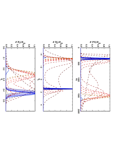
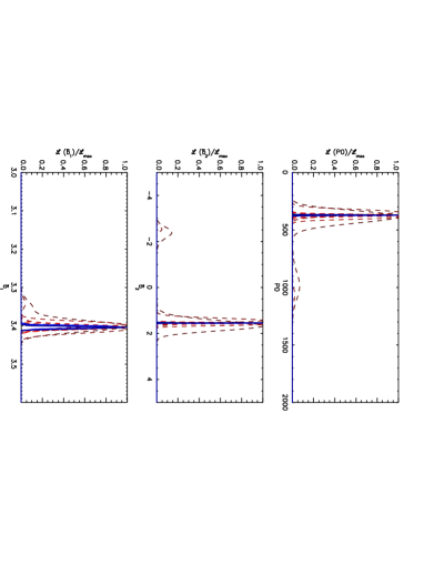
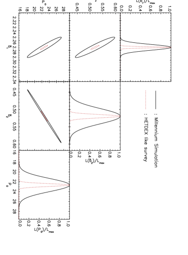
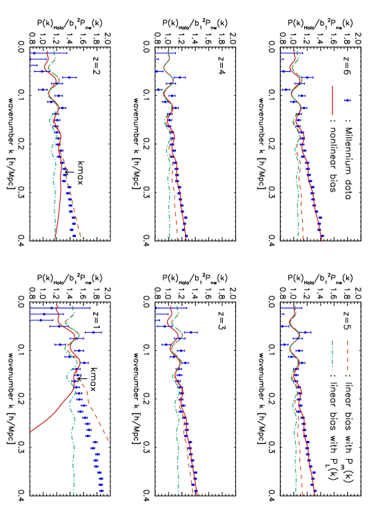
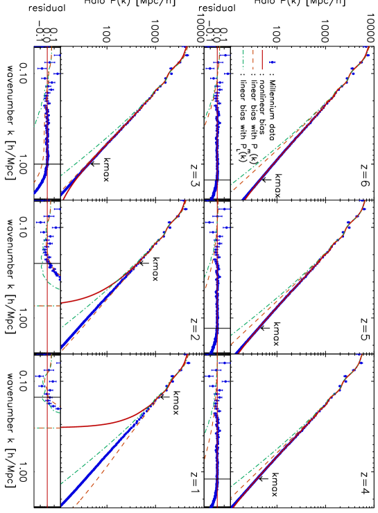
Figure 5 shows the best-fitting non-linear (solid lines) and linear bias models (dashed and dot-dashed lines), compared with the halo spectra estimated from the Millennium Simulation (points with errorbars). The smaller panels show the residuals of fits. The maximum wavenumber used in the fits, $k_{max}(z)$, are also marked with the arrows (bigger panels), and the vertical lines (smaller panels). We find that the non-linear bias model provides substantially better fits than the linear bias models.

We find that all of non-linear bias parameters, $\tilde{b}_{1}$, $\tilde{b}_{2}$, and $P_{0}$, are strongly degenerate, when the maximum wavenumbers used in the fits, $k_{max}$, are small. In Figure 6 we show the one-dimensional marginalized distribution of bias parameters at $z=6$, as a function of $k_{max}$. For lower $k_{max}$, $0.3\leq k_{max}/[h~{}\mathrm{Mpc}^{-1}]\leq 1.0$, the marginalized distribution has two peaks (dashed lines), indicating strong degeneracy with the other parameters. The double-peak structure disappears for $1.0<k_{max}/[h~{}\mathrm{Mpc}^{-1}]\leq 1.5$ (solid lines).

We find that the origin of degeneracy is simply due to the small box size of the Millennium Simulation, i.e., the lack of statistics, or too a large sampling variance. To show this, we have generated a mock Monte Carlo realization of halo power spectra, assuming a much bigger box size, $L_{box}=1.5~{}h^{-1}~{}\mathrm{Gpc}$, which gives the fundamental frequency of $\Delta k=5.0\times 10^{-4}~{}h~{}\mathrm{Mpc}^{-1}$. Note that this volume roughly corresponds to that would be surveyed by the HETDEX survey (Hill et al., 2004). We have used the same non-linear matter power spectrum and the best-fitting bias parameters from the Millennium Simulation (MPA halos) when creating Monte Carlo realizations. The resulting marginalized likelihood function at $z=6$ is shown in Figure 7. The double-peak structure has disappeared even for low $k_{max}$, $k_{max}=0.3~{}h~{}\mathrm{Mpc}^{-1}$. Therefore, we conclude that the double-peak problem can be resolved simply by increasing the survey volume.

The best-fitting non-linear halo bias parameters and the corresponding 1-$\sigma$ intervals are summarized in Table 3. Since we know that the double-peak structure is spurious, we pick one peak that corresponds to the maximum likelihood value, and quote the 1-$\sigma$ interval. At $z\leq 2$, the bias parameters are not constrined very well because of lower $k_{max}$ and the limited statistics of the Millennium Simulation, and hence the two peaks are blended; thus, we estimate 1-$\sigma$ range only from the unblended side of the marginalized likelihood function. Two linear bias parameters, one with the linear matter power spectrum and another with the non-linear PT matter power spectrum, are also presented with their 1-$\sigma$ intervals.

4.2.2 Degeneracy of bias parameters

In order to see how strongly degenerate bias parameters are, we calculate the covariance matrix of each pair of bias parameters. We calculate the covariance matrix of each pair of bias parameters by using the Fisher information matrix, which is the inverse of the covariance matrix. The Fisher information matrix for the galaxy power spectrum can be approximated as (Tegmark, 1997)

$$F_{ij}=\sum_{n}\frac{1}{\sigma_{P}^{2}(k_{n})}\frac{\partial P(k_{n},\mathbf{\theta})}{\partial\theta_{i}}\frac{\partial P(k_{n},\mathbf{\theta})}{\partial\theta_{j}}$$ (9)

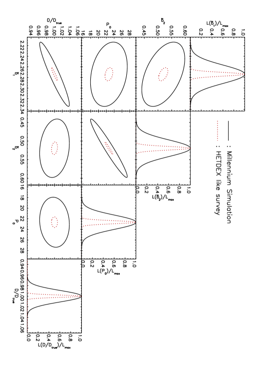
where $\mathbf{\theta}$ is a vector in the parameter space, $\theta_{i}=\tilde{b}_{1}$, $\tilde{b}_{2}$ ,$P_{0}$, for $i=1$, $2$, $3$, respectively. We calculate the marginalized errors on the bias parameters as following. We first calculate the full Fisher matrix and invert it to estimate the covariance matrix. Then, we get the the covariance matrices of any pairs of bias parameters by taking the $2$ by $2$ submatrix of the full covariance matrix. Figure 8 shows the resulting 2-$\sigma$ ($95.45\%$ interval) contour for the bias parameters at $z=4$. We find the strong degeneracy between $\tilde{P}_{0}$ and $\tilde{b}_{2}$. We also find that $\tilde{b}_{1}$ is degenerate with the other two parameters. On top of the error contours for the Millennium Simulation, we show the expected contour from the HETDEX like survey ($1.5~{}\mathrm{Gpc}/h$). Since the volume of HETDEX like survey is 27 times bigger, the likelihood functions and the error-contours are about a factor of 5 smaller than those from the Millennium Simulation. Other than that, two contours follow the same trend. Results are the same for the other redshifts.

4.2.3 Comparison with the halo model predictions

The effective linear bias, $\tilde{b}_{1}$, is larger at higher redshifts. This is the expected result, as halos of mass greater than $\sim 10^{10}M_{\odot}$ were rarer in the earlier time, resulting in the larger bias.

From the same reason, we expect that the non-linear bias parameters, $\tilde{b}_{2}$ and $P_{0}$, are also larger at higher $z$. While we observe the expected trend at $z\geq 4$, the results from $z\leq 3$ are somewhat peculiar. This is probably due to the large sampling variance making the fits unstable: for $z\leq 3$ the maximum wavenumbers inferred from the matter power spectra are less than $1.0~{}h~{}\mathrm{Mpc}^{-1}$ (see Table 1), which makes the likelihood function double-peaked and leaves the bias parameters poorly constrained.

How do these bias parameters compare with the expected values? We use the halo model for computing the mass-averaged bias parameters, $b_{1}^{ST}$ and $b_{2}^{ST}$, assuming that the minimum mass is given by the minimum mass of the MPA halo catalogue, $M_{min}=1.72\times 10^{10}M_{\odot}/h$:

$$b_{i}^{ST}=\frac{\int_{M_{min}}^{M_{max}}\frac{dn}{dM}Mb_{i}(M)dM}{\int_{M_{min}}^{M_{max}}\frac{dn}{dM}MdM},$$ (10)

where $dn/dM$ is the Sheth-Tormen mass function and $b_{i}(M)$ is the $i$-th order bias parameter from Scoccimarro et al. (2001).

There is one subtlety. The halo model predicts the coefficients of the Taylor series (Eq. (1)), whereas what we have measured are the re-parametrized bias parameters given by Eq. (2.2). However, the formula for $\tilde{b}_{1}$ includes the mass variance, $\sigma^{2}$, which depends on our choice of a smoothing scale that is not well defined. This shows how difficult it is to actually compute the halo power spectrum from the halo model. While the measured values of $\tilde{b}_{1}$ and the predicted $b_{1}^{ST}$ compare reasonably well, it is clear that we cannot use the predicted bias values for doing cosmology.

For $\tilde{b}_{2}$, we compute $\tilde{b}_{2}^{ST}=b_{2}^{ST}/\tilde{b}_{1}$ where $\tilde{b}_{1}$ is the best-fitting value from the Millennium Simulation. This would give us a semi apple-to-apple comparison. Nevertheless, while the agreement is reasonable at $z\geq 4$, the halo model predictions should not be used for predicting $\tilde{b}_{2}$ either.

4.2.4 Comments on the bispectrum

While the degeneracy between bias parameters may appear to be a serious issue, there is actually a powerful way of breaking degeneracy: the bispectrum, the Fourier transform of the 3-point correlation function (Matarrese et al., 1997). The reduced bispectrum, which is the bispectrum normalized properly by the power spectrum, depends primarily on two bias parameters, $\tilde{b}_{1}$ and $\tilde{b}_{2}$, nearly independent of the cosmological parameters (Sefusatti et al., 2006). Therefore, one can use this property to fix the bias parameters, and use the power spectrum for determining the cosmological parameters and the remaining bias parameter, $P_{0}$. Sefusatti & Komatsu (2007) have shown that the planned high-$z$ galaxy surveys would be able to determine $\tilde{b}_{1}$ and $\tilde{b}_{2}$ with a few percent accuracy.

We have begun studying the bispectrum of the Millennium Simulation. Our preliminary results show that we can indeed obtain better constraints on $\tilde{b}_{1}$ and $\tilde{b}_{2}$ from the bispectrum than from the power spectrum, provided that we use the same $k_{max}$ for both the bispectrum and power spectrum analyses. Therefore, even when the non-linear bias parameters are poorly constrained by the power spectrum alone, or have the double-peak likelihood function from the power spectrum for lower $k_{max}$, we can still find tight constraints on $\tilde{b}_{1}$ and $\tilde{b}_{2}$ from the bispectrum. These results will be reported elsewhere.

4.2.5 Effects on BAOs

In Figure 9 we show the distortion of BAO features due to non-linear matter clustering and non-linear bias. To show only the distortions of BAOs at each redshift, we have divided the halo power spectra by smooth power spectra without baryonic oscillations from equation (29) of Eisenstein & Hu (1998) with $\tilde{b}_{1}^{2}$ multiplied. Three theoretical models are shown: the non-linear bias model (solid line), a linear bias model with the 3rd-order matter power spectrum (dashed line), and a linear bias model with the linear matter power spectrum (dot-dashed line). Therefore, the difference between the solid lines and the dashed lines is solely due to non-linear halo bias.

The importance of non-linear bias affecting BAOs grows with $z$; however, as the matter clustering is weaker at higher $z$, the 3rd-order PT still performs better than at lower $z$. In other words, the higher bias at higher $z$ does not mean that surveys at higher $z$ are worse at measuring BAOs; on the contrary, it is still easier to model the halo power spectrum at higher $z$ than at lower $z$. For $z\geq 3$, where $k_{max}$ is larger than the BAO scale, the distortion of BAOs is modeled very well by the non-linear bias model, while the linear bias models fail badly.

The sampling variance of the Millennium Simulation at $k\lesssim 0.15~{}h~{}{\rm Mpc}^{-1}$ is too large for us to study the distortion on the first two BAO peaks. Since the PT performs well at higher $k$, we expect that the PT describes the first two peaks even better. However, to show this explicitly one would need to run a bigger simulation with a bigger volume with the same mass resolution as the Millennium Simulation, which should be entirely doable with the existing computing resources.

4.3. Galaxy power spectra

4.3.1 Measuring non-linear galaxy bias parameters

Figure 10.— Same as Figure 5, but for the MPA galaxy catalogue (Mgalaxy).

Figure 11.— Same as Figure 5, but for the Durham galaxy catalogue (Dgalaxy).

Table 4Non-linear halo bias parameters and the corresponding 68% interval estimated from the MPA galaxy power spectra

$z$	$\tilde{b}_{1}$	$\tilde{b}_{2}$	$P_{0}$	$b_{1}^{L}$	$b_{1}^{LL}$	$b_{1}^{ST}$	$\tilde{b}_{2}^{ST}$
			($[h/\mathrm{Mpc}]^{3}$)
6	3.55$\pm$0.01	1.70$\pm$0.03	194.23$\pm$4.45	3.67$\pm$0.03	3.68$\pm$0.03	3.10	1.03
5	2.93$\pm$0.01	1.08$\pm$0.03	94.08$\pm$3.71	2.97$\pm$0.03	2.98$\pm$0.03	2.55	0.59
4	2.46$\pm$0.01	0.68$\pm$0.03	47.79$\pm$2.84	2.47$\pm$0.02	2.48$\pm$0.02	2.13	0.28
3	1.69$\pm$0.01	-2.12$\pm$0.04	486.69$\pm$12.7	1.83$\pm$0.02	1.83$\pm$0.02	1.58	-0.12
2	1.28$\pm$0.08	-2.16$\pm$0.64	738.22$\pm$291.3	1.40$\pm$0.01	1.40$\pm$0.01	1.19	-0.34
1	0.89$\pm$0.11	-2.97$\pm$1.60	2248.35$\pm$786.13	1.09$\pm$0.01	1.10$\pm$0.01	0.91	-0.45

Note. — $z$: redshift

$\tilde{b}_{1}$, $\tilde{b}_{2}$, $P_{0}$: non-linear bias parameters

$b_{1}^{L}$: linear bias parameter for the linear bias model with the 3rd-order matter power spectrum

$b_{1}^{LL}$: linear bias parameter for the linear bias model with the linear power spectrum

$b_{1}^{ST}$, $\tilde{b}_{2}^{ST}$: non-linear bias parameters calculated from the Sheth-Tormen model, $\tilde{b}_{2}^{ST}$=$b_{2}^{ST}/\tilde{b}_{1}$

Caution: We estimate 1-$\sigma$ ranges for the low redshift ($z\leq 3$) only for the peak which involves the maximum likelihood value. If two peaks in maginalized likelihood function are blended, we use only unblended side of the peak to estimate the 1-$\sigma$ range.

Table 5Non-linear halo bias parameters and the corresponding 68% interval estimated from the Durham galaxy power spectra

$z$	$\tilde{b}_{1}$	$\tilde{b}_{2}$	$P_{0}$	$b_{1}^{L}$	$b_{1}^{LL}$	$b_{1}^{ST}$	$\tilde{b}_{2}^{ST}$
			($[h/\mathrm{Mpc}]^{3}$)
6	3.73$\pm$0.01	1.96$\pm$0.03	288.39$\pm$5.82	3.90$\pm$0.04	3.90$\pm$0.04	3.10	0.98
5	3.07$\pm$0.01	1.26$\pm$0.03	143.15$\pm$4.81	3.15$\pm$0.03	3.15$\pm$0.03	2.55	0.56
4	2.57$\pm$0.01	0.83$\pm$0.03	78.97$\pm$3.93	2.60$\pm$0.02	2.61$\pm$0.02	2.13	0.26
3	1.75$\pm$0.01	-2.26$\pm$0.04	604.65$\pm$13.8	1.92$\pm$0.02	1.93$\pm$0.02	1.58	-0.11
2	1.36$\pm$0.08	-2.14$\pm$0.65	843.49$\pm$331.4	1.49$\pm$0.01	1.50$\pm$0.01	1.19	-0.32
1	0.96$\pm$0.11	-2.94$\pm$1.62	2640.20$\pm$960.32	1.18$\pm$0.01	1.20$\pm$0.01	0.91	-0.42

Note. — $z$: redshift

$\tilde{b}_{1}$, $\tilde{b}_{2}$, $P_{0}$: non-linear bias parameters

$b_{1}^{L}$: linear bias parameter for the linear bias model with the 3rd-order matter power spectrum

$b_{1}^{LL}$: linear bias parameter for the linear bias model with the linear power spectrum

$b_{1}^{ST}$, $\tilde{b}_{2}^{ST}$: non-linear bias parameters calculated from the Sheth-Tormen model, $\tilde{b}_{2}^{ST}$=$b_{2}^{ST}/\tilde{b}_{1}$

Caution: We estimate 1-$\sigma$ ranges for the low redshift ($z\leq 3$) only for the peak which involves the maximum likelihood value. If two peaks in maginalized likelihood function are blended, we use only unblended side of the peak to estimate the 1-$\sigma$ range.

Figure 12.— Same as Figure 9, but for the MPA galaxy power spectrum (Mgalaxy).

Figure 13.— Same as Figure 9, but for the Durham galaxy power spectrum (Dgalaxy).

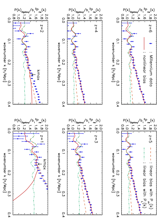
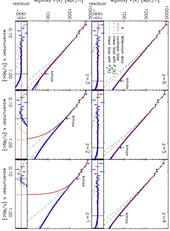
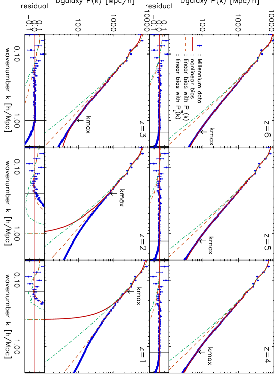
Figures 10 and 11 show the galaxy power spectra estimated from the MPA (Mgalaxy) and Durham (Dgalaxy) galaxy catalogues, respectively. Here, we basically find the same story as we have found for the halo power spectra (§ 4.2): for $k<k_{max}$ the non-linear bias model fits both galaxy power spectra (Mgalaxy and Dgalaxy), whereas the linear bias models fit neither.

The galaxy bias parameters extracted from Mgalaxy and Dgalaxy are summarized in Table 4 and 5, respectively. While the bias parameters are different for halo, Mgalaxy and Dgalaxy, they follow the same trend: (i) $\tilde{b}_{1}$ becomes lower as the redshift becomes lower, and (ii) $\tilde{b}_{2}$ also becomes lower as the redshift becomes lower when $z>3$, but suddenly changes to large negative values at $z\leq 3$. As we have already pointed out in § 4.2, this sudden peculiar change is most likely caused by the double-peak nature of the likelihood function, owing to the poor statistical power for lower $k_{max}$ at lower $z$. In order to study $\tilde{b}_{2}$ further with better statistics, one needs a bigger simulation.

4.3.2 Comparison with the simplest HOD predictions

To give a rough theoretical guide for the galaxy bias parameters, we assume that each dark matter halo hosts one galaxy above a certain minimum mass. This specifies the form of the HOD completely: $\langle N|M\rangle=1$, with the same lower mass cut-off as the minimum mass of the halo, $M_{min}=1.72\times 10^{10}M_{\odot}/h$.

This is utterly simplistic, and is probably not correct for describing Mgalaxy or Dgalaxy. Nevertheless, we give the resulting values in Table 4 and 5, which have been computed from

$$b_{i}^{ST}=\frac{\int_{M_{min}}^{M_{max}}\frac{dn}{dM}b_{i}(M)\langle N|M\rangle dM}{\int_{M_{min}}^{M_{max}}\frac{dn}{dM}\langle N|M\rangle dM},$$ (11)

where $dn/dM$ is the Sheth-Tormen mass function and $b_{i}(M)$ is the $i$-th order bias parameter from Scoccimarro et al. (2001). To compare with the non-linear bias parameters, we also calculate $\tilde{b}_{2}=b_{2}^{ST}/\tilde{b}_{1}$.

While these “predictions” give values that are reasonably close to the ones obtained from the fits, they are many $\sigma$ away from the best-fitting values. The freedom in the choice of the HOD may be used to make the predicted values match the best-fitting values; however, such an approach would require at least as many free parameters as the non-linear bias parameters. Also, given that the halo bias prediction fails to fit the halo power spectra, the HOD approach, which is still based upon knowing the halo bias, is bound to fail as well.

4.3.3 Effects on BAOs

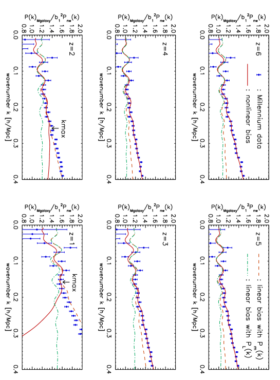
In Figures 12 and 13 we show how non-linear galaxy bias distorts the structure of BAOs. Again, we find the same story as we have found for the halo bias: the galaxy bias distorts BAOs more at higher $z$ because, for a given mass, galaxies were rarer at higher redshifts and thus more highly biased, while the quality of the fits is better at higher $z$ because of less non-linearity in the matter clustering.

In all cases (halo, Mgalaxy and Dgalaxy) the non-linear bias model given by Eq. (2) provides very good fits, and describes how bias modifies BAOs.

4.4. Mass dependence of bias parameters and effects on BAOs

Figure 14.— Mass dependence of distortion of BAOs due to non-linear bias. Four mass bins, $M<5\times 10^{10}M_{\odot}/h$, $5\times 10^{10}M_{\odot}/h<M<10^{11}M_{\odot}/h$, $10^{11}M_{\odot}/h<M<5\times 10^{11}M_{\odot}/h$, and $5\times 10^{11}M_{\odot}/h<M<10^{12}M_{\odot}/h$, are shown. ($M_{10}$ stands for $M/(10^{10}M_{\sun})$.) All of the power spectra have been divided by a smooth power spectrum without baryonic oscillations from equation (29) of Eisenstein & Hu (1998). The errorbars show the Millennium Simulation data, while the solid lines show the PT calculation.

Figure 15.— Same as Figure 14, but for the MPA galaxy catalogue (Mgalaxy).

Table 6Mass dependence of non-linear halo bias parameters (MPA halos)

$z$	$\mathrm{M_{min}}$	$\mathrm{M_{max}}$	$\tilde{b}_{1}$	$\tilde{b}_{2}$	$P_{0}$	$b_{1}^{ST}$	$\tilde{b}_{2}^{ST}$
	($M_{\odot}/h$)	($M_{\odot}/h$)			($[h/\mathrm{Mpc}]^{3}$)
6	1.7E+10	5.0E+10	3.19$\pm$0.01	1.28$\pm$0.03	88.76$\pm$2.97	2.96	0.93
	5.0E+10	1.0E+11	3.90$\pm$0.02	1.91$\pm$0.04	288.18$\pm$8.02	3.52	1.36
	1.0E+11	5.0E+11	4.66$\pm$0.03	3.04$\pm$0.05	1029.19$\pm$18.84	4.41	2.28
	5.0E+11	1.0E+12	6.41$\pm$0.14	5.76$\pm$0.21	6910.17$\pm$200.74	5.95	3.59
5	1.7E+10	5.0E+10	2.55$\pm$0.01	0.71$\pm$0.03	31.51$\pm$2.06	2.41	0.48
	5.0E+10	1.0E+11	3.09$\pm$0.01	1.19$\pm$0.04	120.84$\pm$5.69	2.84	0.81
	1.0E+11	5.0E+11	3.78$\pm$0.02	1.79$\pm$0.04	402.11$\pm$12.40	3.55	1.48
	5.0E+11	1.0E+12	5.14$\pm$0.07	3.55$\pm$0.11	2805.48$\pm$94.53	4.71	2.44
4	1.7E+10	5.0E+10	2.08$\pm$0.01	0.38$\pm$0.04	10.90$\pm$1.19	2.01	0.15
	5.0E+10	1.0E+11	2.51$\pm$0.01	0.66$\pm$0.04	42.34$\pm$3.52	2.33	0.40
	1.0E+11	5.0E+11	3.05$\pm$0.01	1.08$\pm$0.04	161.22$\pm$8.11	2.90	0.92
	5.0E+11	1.0E+12	3.80$\pm$0.05	-4.08$\pm$0.09	3431.19$\pm$64.81	3.79	1.77
3	1.7E+10	5.0E+10	1.39$\pm$0.01	-1.83$\pm$0.05	241.59$\pm$9.58	1.47	-0.25
	5.0E+10	1.0E+11	1.75$\pm$0.01	0.11$\pm$0.05	2.48$\pm$0.29	1.67	-0.10
	1.0E+11	5.0E+11	2.09$\pm$0.01	0.35$\pm$0.04	20.95$\pm$3.22	2.04	0.19
	5.0E+11	1.0E+12	2.78$\pm$0.02	0.82$\pm$0.06	171.31$\pm$21.03	2.57	0.60
2	1.7E+10	5.0E+10	1.01$\pm$0.05	-1.98$\pm$0.68	373.60$\pm$149.24	1.11	-0.46
	5.0E+10	1.0E+11	1.14$\pm$0.07	-2.30$\pm$0.63	627.69$\pm$204.69	1.23	-0.40
	1.0E+11	5.0E+11	1.31$\pm$0.08	-2.34$\pm$0.63	869.30$\pm$272.06	1.44	-0.28
	5.0E+11	1.0E+12	1.62$\pm$0.11	-2.53$\pm$0.69	1566.40$\pm$476.07	1.75	-0.05
1	1.7E+10	5.0E+10	0.68$\pm$0.09	-3.12$\pm$1.46	1315.40$\pm$447.14	0.86	-0.58
	5.0E+10	1.0E+11	0.75$\pm$0.10	-3.24$\pm$1.46	1699.76$\pm$571.75	0.92	-0.56
	1.0E+11	5.0E+11	0.85$\pm$0.09	-2.80$\pm$1.65	1783.07$\pm$683.57	1.02	-0.53
	5.0E+11	1.0E+12	0.99$\pm$0.11	-2.82$\pm$1.95	2443.76$\pm$972.16	1.17	-0.47

Note. — $z$: redshift

$\mathrm{M_{min}}$: minimum mass for a given bin

$\mathrm{M_{max}}$: maximum mass for a given bin

$\tilde{b}_{1}$, $\tilde{b}_{2}$, $P_{0}$: non-linear bias parameters

$b_{1}^{ST}$, $\tilde{b}_{2}^{ST}$: bias parameters from the Sheth-Tormen model, $\tilde{b}_{2}^{ST}$=$b_{2}^{ST}/\tilde{b}_{1}$

Caution: We estimate 1-$\sigma$ ranges for the low redshift ($z\leq 3$) only for the peak which involves the maximum likelihood value. If two peaks in maginalized likelihood function are blended, we use only unblended side of the peak to estimate the 1-$\sigma$ range.

Table 7Mass dependence of non-linear galaxy bias parameters (MPA galaxies)

$z$	$\mathrm{M_{min}}$	$\mathrm{M_{max}}$	$\tilde{b}_{1}$	$\tilde{b}_{2}$	$P_{0}$	$b_{1}^{ST}$	$\tilde{b}_{2}^{ST}$
	($M_{\odot}/h$)	($M_{\odot}/h$)			($[h/\mathrm{Mpc}]^{3}$)
6	1.7E+10	5.0E+10	3.37$\pm$0.01	1.50$\pm$0.03	136.39$\pm$3.69	2.91	0.82
	5.0E+10	1.0E+11	3.96$\pm$0.02	2.00$\pm$0.04	325.38$\pm$8.44	3.49	1.31
	1.0E+11	5.0E+11	4.69$\pm$0.03	3.09$\pm$0.05	1078.72$\pm$19.25	4.23	2.01
	5.0E+11	1.0E+12	6.43$\pm$0.14	5.79$\pm$0.20	7046.28$\pm$201.94	5.89	3.49
5	1.7E+10	5.0E+10	2.77$\pm$0.01	0.93$\pm$0.03	63.17$\pm$2.99	2.38	0.40
	5.0E+10	1.0E+11	3.16$\pm$0.01	1.27$\pm$0.04	144.20$\pm$6.16	2.82	0.77
	1.0E+11	5.0E+11	3.81$\pm$0.02	1.84$\pm$0.04	432.51$\pm$12.80	3.41	1.28
	5.0E+11	1.0E+12	5.15$\pm$0.07	3.60$\pm$0.11	2897.95$\pm$95.17	4.67	2.37
4	1.7E+10	5.0E+10	2.33$\pm$0.01	0.58$\pm$0.03	32.25$\pm$2.25	1.98	0.11
	5.0E+10	1.0E+11	2.59$\pm$0.01	0.74$\pm$0.04	56.91$\pm$4.08	2.32	0.37
	1.0E+11	5.0E+11	3.09$\pm$0.02	1.13$\pm$0.04	179.81$\pm$8.52	2.79	0.77
	5.0E+11	1.0E+12	3.83$\pm$0.05	-4.09$\pm$0.09	3507.05$\pm$64.85	3.76	1.71
3	1.7E+10	5.0E+10	1.62$\pm$0.01	-2.07$\pm$0.05	431.79$\pm$12.04	1.45	-0.22
	5.0E+10	1.0E+11	1.84$\pm$0.01	0.19$\pm$0.04	7.04$\pm$1.04	1.66	-0.10
	1.0E+11	5.0E+11	2.14$\pm$0.01	0.38$\pm$0.04	27.64$\pm$3.67	1.96	0.12
	5.0E+11	1.0E+12	2.80$\pm$0.02	0.84$\pm$0.06	191.24$\pm$21.65	2.55	0.57
2	1.7E+10	5.0E+10	1.26$\pm$0.07	-2.09$\pm$0.66	683.11$\pm$240.40	1.10	-0.37
	5.0E+10	1.0E+11	1.21$\pm$0.08	-2.35$\pm$0.62	738.09$\pm$231.05	1.22	-0.38
	1.0E+11	5.0E+11	1.35$\pm$0.09	-2.32$\pm$0.63	919.65$\pm$288.79	1.40	-0.29
	5.0E+11	1.0E+12	1.65$\pm$0.11	-2.50$\pm$0.69	1602.17$\pm$480.23	1.74	-0.06
1	1.7E+10	5.0E+10	0.91$\pm$0.11	-2.96$\pm$1.59	2344.13$\pm$802.55	0.86	-0.43
	5.0E+10	1.0E+11	0.79$\pm$0.11	-3.28$\pm$1.51	1956.42$\pm$657.89	0.92	-0.53
	1.0E+11	5.0E+11	0.87$\pm$0.10	-2.88$\pm$1.63	1964.64$\pm$738.71	1.00	-0.51
	5.0E+11	1.0E+12	1.01$\pm$0.11	-2.80$\pm$2.01	2550.21$\pm$1007.23	1.16	-0.46

Note. — $z$: redshift

$\mathrm{M_{min}}$: minimum mass for a given bin

$\mathrm{M_{max}}$: maximum mass for a given bin

$\tilde{b}_{1}$, $\tilde{b}_{2}$, $P_{0}$: non-linear bias parameters

$b_{1}^{ST}$, $\tilde{b}_{2}^{ST}$: bias parameters from the Sheth-Tormen model, $\tilde{b}_{2}^{ST}$=$b_{2}^{ST}/\tilde{b}_{1}$

Caution: We estimate 1-$\sigma$ ranges for the low redshift ($z\leq 3$) only for the peak which involves the maximum likelihood value. If two peaks in maginalized likelihood function are blended, we use only unblended side of the peak to estimate the 1-$\sigma$ range.

So far, we have used all the available halos and galaxies in the Millennium catalogues for computing the halo and galaxy power spectra. In this section we divide the samples into different mass bins given by $M<5\times 10^{10}M_{\odot}/h$, $5\times 10^{10}M_{\odot}/h<M<10^{11}M_{\odot}/h$, $10^{11}M_{\odot}/h<M<5\times 10^{11}M_{\odot}/h$, $5\times 10^{11}M_{\odot}/h<M<10^{12}M_{\odot}/h$, and study how the derived bias parameters depend on mass.

The power spectra of the selected halos and galaxies in a given mass bin are calculated and fit in the exactly same manner as before. Note that we shall use only the halo and Mgalaxy, as we expect that Dgalaxy would give similar results to Mgalaxy.

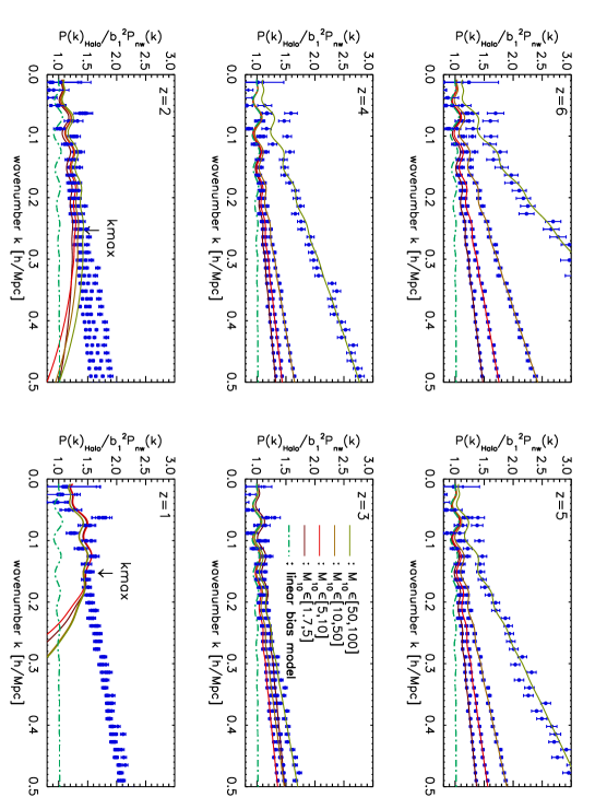
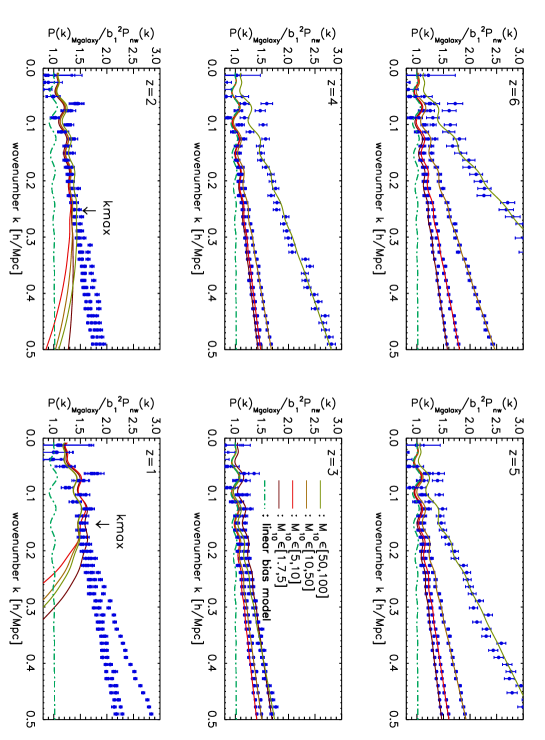
Figures 14 and 15 show the results for the halo and galaxies, respectively. To compare the power spectra of different mass bins in the same panel, and highlight the effects on BAOs at the same time, we have divided the power spectra by a non-oscillating matter power spectrum from equation (29) of Eisenstein & Hu (1998) with the best-fitting $\tilde{b}_{1}^{2}$ from each mass bin multiplied. These figures show the expected results: the larger the mass is, the larger the non-linear bias becomes. Nevertheless, the 3rd-order PT calculation captures the dependence on mass well, and there is no evidence for failure of the PT for highly biased objects.

In Tables 6 and 7 we give values of the measured bias parameters as well as the “predicted” values. For all redshifts we see the expected trend again: the higher the mass is, the larger the effective linear bias ($\tilde{b}_{1}$) is. The same is true for $\tilde{b}_{2}$ for $z>3$, while it is not as apparent for lower redshifts, and eventually becomes almost fuzzy for $z=1$. Again, these are probably due to the lack of statistics due to lower values of $k_{max}$ at lower $z$, and we need a bigger simulation to handle these cases with more statistics.

The high values of bias do not mean failure of PT. The PT galaxy power spectrum model fails only when $\Delta^{2}_{m}(k,z)$ exceeds $\sim 0.4$ (Paper I), or the locality of bias is violated. Overall, we find that the non-linear bias model given by Eq. (2) performs well for halos and galaxies with all mass bins, provided that we use the data only up to $k_{max}$ determined from the matter power spectra. This implies that the locality assumption is a good approximation for $k<k_{max}$; however, is it good enough for us to extract cosmology from the observed galaxy power spectra?

5. Cosmological parameter estimation with the non-linear bias model

In the previous sections we have shown that the 3rd-order PT galaxy power spectrum given by Eq. (2) provides good fits to the galaxy power spectrum data from the Millennium Simulation.

However, we must not forget that Eq. (2) contains 3 free parameters, $\tilde{b}_{1}$, $\tilde{b}_{2}$, and $P_{0}$. With 3 parameters it may seem that it should not be so difficult to fit smooth curves like those shown in, e.g., Figure 10.

While the quality of fits is important, it is not the end of story. We must also show that Eq. (2) can be used for extracting the correct cosmological parameters from the observed galaxy power spectra.

In this section we shall extract the distance scale from the galaxy power spectra of the Millennium Simulation, and compare them with the input values that were used to generate the simulation. If they do not agree, Eq. (2) must be discarded. If they do, we should proceed to the next level by including non-linear redshift space distortion.

5.1. Measuring Distance Scale

5.1.1 Background

Dark energy influences the expansion rate of the universe as well as the growth of structure (see Copeland et al., 2006, for a recent review).

The cosmological distances, such as the luminosity distance, $D_{L}(z)$, and angular diameter distance, $D_{A}(z)$, are powerful tools for measuring the expansion rates of the universe, $H(z)$, over a wide range of redshifts. Indeed, it was $D_{L}(z)$ measured out to high-$z$ ($z\leq 1.7$) Type Ia supernovae that gave rise to the first compelling evidence for the existence of dark energy (Riess et al., 1998; Perlmutter et al., 1999). The CMB power spectrum provides us with a high-precision measurement of $D_{A}(z_{*})$ out to the photon decoupling epoch, $z_{*}\simeq 1090$ (see Komatsu et al., 2008, for the latest determination from the WMAP 5-year data).

The galaxy power spectrum can be used for measuring $D_{A}(z)$ as well as $H(z)$ over a wider range of redshifts. From galaxy surveys we find three-dimensional positions of galaxies by measuring their angular positions on the sky as well as their redshifts. We can then estimate the two-point correlation function of galaxies as a function of the angular separation, $\Delta\theta$, and the redshift separation, $\Delta z$. To convert $\Delta\theta$ and $\Delta z$ into the comoving separations perpendicular to the line of sight, $\Delta r_{\perp}$, and those along the line of sight, $\Delta r_{\parallel}$, one needs to know $D_{A}(z)$ and $H(z)$, respectively, as

$$\Delta r_{\perp} = (1+z)D_{A}(z)\Delta\theta,$$ (12)

$$\Delta r_{\parallel} = \frac{c\Delta z}{H(z)},$$ (13)

where $(1+z)$ appears because $D_{A}(z)$ is the proper (physical) angular diameter distance, whereas $\Delta r_{\perp}$ is the comoving separation. Therefore, if we know $\Delta r_{\perp}$ and $\Delta r_{\parallel}$ a priori, then we may use the above equations to measure $D_{A}(z)$ and $H(z)$.

The galaxy power spectra contain at least three distance scales which may be used in the place of $\Delta r_{\perp}$ and $\Delta r_{\parallel}$: (i) the sound horizon size at the so-called baryon drag epoch, $z_{drag}\simeq 1020$, at which baryons were released from the baryon-photon plasma, (ii) the photon horizon size at the matter-radiation equality, $z_{eq}\simeq 3200$, and (iii) the Silk damping scale (see, e.g., Eisenstein & Hu, 1998).

In Fourier space, we may write the observed power spectrum as (Seo & Eisenstein, 2003)

$$P_{obs} ( k_{\parallel},k_{\perp},z)=\left(\frac{D_{A}(z)}{D_{A,\mathrm{true}}(z)}\right)^{2}\left(\frac{H_{\mathrm{true}}(z)}{H(z)}\right)$$ (14)

$$\times P_{\mathrm{true}}\left(\frac{D_{A,\mathrm{true}}(z)}{D_{A}(z)}k_{\perp},\frac{H(z)}{H_{\mathrm{true}}(z)}k_{\parallel},z\right),$$

where $k_{\perp}$ and $k_{\parallel}$ are the wavenumbers perpendicular to and parallel to the line of sight, respectively, and $P_{true}(k)$, $D_{A,true}(z)$, and $H_{true}(z)$ are the true, underlying values. We then vary $D_{A}(z)$ and $H(z)$, trying to estimate $D_{A,true}(z)$ and $H_{true}(z)$.

There are two ways of measuring $D_{A}(z)$ and $H(z)$ from the galaxy power spectra:

• Use BAOs. The BAOs contain the information of one of the standard rulers, the sound horizon size at $z_{drag}$. This method relies on measuring only the phases of BAOs, which are markedly insensitive to all the non-linear effects (clustering, bias, and redshift space distortion) (Seo & Eisenstein, 2005; Eisenstein et al., 2007; Nishimichi et al., 2007; Smith et al., 2008; Angulo et al., 2008; Sanchez et al., 2008; Seo et al., 2008; Shoji et al., 2008), despite the fact that the amplitude is distorted by non-linearities (see Figures 4, 9, 12, and 13). Therefore, BAOs provide a robust means to measure $D_{A}(z)$ and $H(z)$, and they have been used for determining $D_{A}^{2}H^{-1}$ out to $z=0.2$ from the SDSS main galaxy sample and 2dFGRS, as well as to $z=0.35$ from the SDSS Luminous Red Galaxy (LRG) sample (Eisenstein et al., 2005; Percival et al., 2007); however, since they use only one standard ruler, the constraints on $D_{A}(z)$ and $H(z)$ from the BAO-only analysis are weaker than the full analysis (Shoji et al., 2008).

• Use the entire shpae of the power spectrum. This approach gives the best determination (i.e., the smallest error) of $D_{A}(z)$ and $H(z)$, as it uses all the standard rulers encoded in the galaxy power spectrum; however, one must understand the distortions of the shape of the power spectrum due to non-linear effects. The question is, “is the 3rd-order (or higher) PT good enough for correcting the key non-linear effects?”

In this paper we show, for the first time, that we can extract the distance scale using the 3rd-order PT galaxy power spectrum in real space. While we have not yet included the effects of redshift space distortion, this is a significant step towards extracting $D_{A}(z)$ and $H(z)$ from the entire shape of the power spectrum of galaxies. We shall address the effect of non-linear redshift space distortion in the future work.

5.1.2 Method: Measuring “Box Size” of the Millennium Simulation

In real space simulations (as opposed to redshift space ones), there is only one distance scale in the problem: the box size of the simulation, $L_{\mathrm{box}}$, which is $L_{\mathrm{box}}^{\mathrm{(true)}}=500~{}\mathrm{Mpc}/h$ for the Millennium simulation. Then, “estimating the distance scale from the Millennium Simulation” becomes equivalent to “estimating $L_{\rm box}$ from the Millennium Simulation. Eq. (14) now leads:

$$P_{obs}(k,L_{\mathrm{box}})=\left(\frac{L_{\mathrm{box}}}{L_{\mathrm{box}}^{\mathrm{(true)}}}\right)^{3}P_{\mathrm{true}}\left(\frac{L_{\mathrm{box}}^{\mathrm{(true)}}}{L_{\mathrm{box}}}k\right).$$ (15)

As we estimate the variance of power spectrum from the observed power spectrum, we need to rescale the variance when the normalization of the observed power spectrum changes :

$$\sigma_{Pi}^{2}(L_{\mathrm{box}})=\left(\frac{L_{\mathrm{box}}}{L_{\mathrm{box}}^{\mathrm{(true)}}}\right)^{6}\sigma_{Pi}^{2}(L_{\mathrm{box}}^{\mathrm{(true)}})$$ (16)

We estimate $L_{\mathrm{box}}$ using the likelihood function given by

$$\mathcal{L}(\tilde{b}_{1},\tilde{b}_{2}, P_{0} ,L_{\mathrm{box}})=\prod_{k_{i}<k_{max}}\frac{1}{\sqrt{2\pi\sigma_{Pi}^{2}(L_{\mathrm{box}})}}$$ (17)

$$\times \exp\left[-\frac{\left\{P_{obs}(k_{i}/\alpha)-P_{g}(k_{i}/\alpha)/\alpha^{3}\right\}^{2}}{2\sigma_{P}^{2}(k_{i}/\alpha)}\right],$$

where $\alpha=L_{\mathrm{box}}/L_{\mathrm{box}}^{\mathrm{(true)}}$.

The likelihood function, Eq. (17), still depends upon the bias parameters that we wish to eliminate. Therefore we marginalize the likelihood function over all the bias parameters with flat priors. We obtain (see also Appendix B):

$$\mathcal{L}(L_{\mathrm{box}})=\int_{0}^{\infty}d\tilde{b}_{1}^{2}\int_{-\infty}^{\infty}d\tilde{b}_{2}\int_{-\infty}^{\infty}dP_{0}~{}\mathcal{L}(\tilde{b}_{1},\tilde{b}_{2},P_{0},L_{\mathrm{box}}).$$ (18)

Hereafter, we shall simply call $L_{\mathrm{box}}$ as $D$ for ‘distance scale’. $D$ is closely related to the angular diameter distance, $D_{A}(z)$, and the expansion rate, $H(z)$, in real surveys. (See, §5.1.1)

5.1.3 Results: Unbiased Extraction of the distance scale from the Millennium Simulation

Figure 16.— Distance scale extracted from the Millennium Simulation using the 3rd-order PT galaxy power spectrum given by Eq. (2), divided by the true value. The mean of the likelihood (stars), and the maximum likelihood values (filled circles) and the corresponding 1-$\sigma$ intervals (errorbars), are shown as a function of maximum wavenumbers used in the fits, $k_{max}$. We find $D/D_{true}=1$ to within the 1-$\sigma$ errors from all the halo/galaxy catalogues (“halo,” “Mgalaxy,” and “Dgalaxy”) at all redshifts, provided that we use $k_{max}$ estimated from the matter power spectra, $k_{max}=0.15$, 0.25, 1.0, 1.2, 1.3, and 1.5 at $z=1$, 2, 3, 4, 5, and 6, respectively (see Table 1). Note that the errors on $D$ do not decrease as $k_{max}$ increases due to degeneracy between $D$ and the bias parameters. See Figure (18) and (19) for further analysis.

Figure 17.— Same as Figure 8, but including the distance scale $D/D_{true}$.

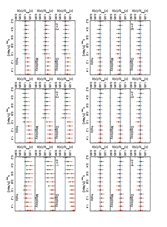
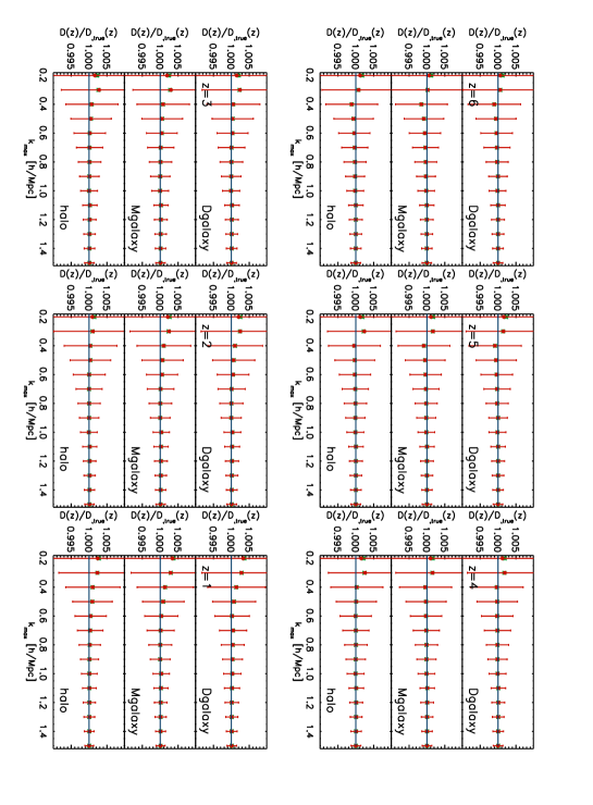
In Figure 16 we show $D(z)/D_{true}(z)$ estimated from the halo, Mgalaxy, and Dgalaxy catalogues at $z=1$, 2, 3, 4, 5, and 6. The maximum likelihood values (filled circles) and the corresponding 1-$\sigma$ intervals (errorbars), as well as the mean of the likelihood (stars) are shown. We find $D(z)/D_{true}(z)=1$ to within the 1-$\sigma$ errors from all of the halo/galaxy catalogues at all redshifts, provided that we use $P_{obs}(k)$ only up to $k_{max}$ that has been determined unambiguously from the matter power spectrum (see Table 1). Not only does this provide a strong support for the validity of Eq. (2), but also it provides a practical means for extracting $D$ from the full shape of the observed galaxy power spectra.

Despite a small volume of the Millennium Simulation and the use of flat priors on the bias parameters upon marginalization, we could determine $D$ to about 2.5% accuracy.

In addition, we also find that the error on $D$ hardly decreases even though $k_{max}$ increases. It is because of the degeneracy between $D$ and the bias parameters. In order to see how strongly degenerate they are, we calculate correlations between pairs of parameters ($\tilde{b}_{1}$,$\tilde{b}_{2}$,$P_{0}$,$D/D_{true}$) by the Fisher information matrix from Eq. (9).

Figure 17 shows both one-dimensional marginalized constraints and two-dimensional joint marginalized constraints of 2-$\sigma$ range ($95.45\%$ CL) for the bias parameters and the distance scale. This figure indicates that when we include the distance scale, the correlations between bias parameters become milder. It is mainly due to the correlation between the distance scale and $\tilde{b}_{1}$ making the constraint on $\tilde{b}_{1}$ weaker. On the other hand, the one-dimensional marginalized likelihood functions for $\tilde{b}_{2}$ and $P_{0}$ are hardly changed. The remaining degeneracies are those between ($\tilde{b}_{2}$,$P_{0}$) and ($\tilde{b}_{1}$,$D/D_{true}$). These degeneracies would be broken when we include the information from the bispectrum, as the bispectrum will measure $\tilde{b}_{1}$ and $\tilde{b}_{2}$.

5.1.4 Optimal estimation of the distance scale

Figure 18.— Same as Figure 16, but with $\tilde{b}_{1}$ and $\tilde{b}_{2}$ fixed at the best-fitting values. The 1-$\sigma$ ranges for $D$ are $1.5\%$ and $0.15\%$ for $k_{max}=0.2~{}h/\mathrm{Mpc}$ and $k_{max}=1.5~{}h/\mathrm{Mpc}$, respectively. The errors on $D$ decrease as $k_{max}$ increases, but the scaling is still milder than $1/\sqrt{\sum_{k<k_{max}}N_{k}}$.

Figure 19.— Same as Figure 16, but with $\tilde{b}_{1}$, $\tilde{b}_{2}$ and $P_{0}$ fixed at the best-fitting values. The 1-$\sigma$ ranges for $D$ are $0.8\%$ and $0.05\%$ for $k_{max}=0.2~{}h/\mathrm{Mpc}$ and $k_{max}=1.5~{}h/\mathrm{Mpc}$, respectively. The errors on $D$ decrease as $k_{max}$ increases as $1/\sqrt{\sum_{k<k_{max}}N_{k}}$.

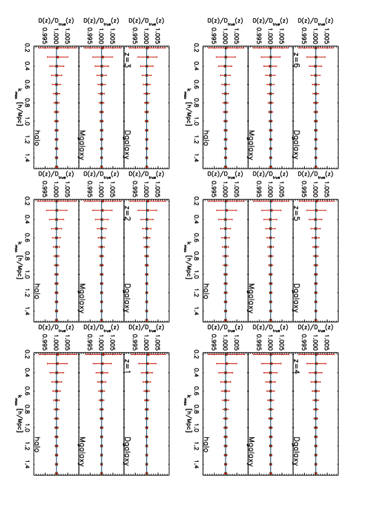
The constraint we find from the previous subsection will get better when we include the bispectrum, as the reduced bispectrum provides independent and strong constraints on $\tilde{b}_{1}$ and $\tilde{b}_{2}$ (Sefusatti et al., 2006).

How much will it be better? First, let us assume that we know the exact values of $\tilde{b}_{1}$ and $\tilde{b}_{2}$. In this case, we get the error on $D$ by marginalizing only over $P_{0}$ while setting $\tilde{b}_{1}$ and $\tilde{b}_{2}$ to be the best-fitting values, i.e.

$$\mathcal{L}^{\mathrm{fix}~{}\tilde{b}_{1}\tilde{b}_{2}}(D)=\int_{-\infty}^{\infty}dP_{0}\mathcal{L}(\tilde{b}_{1}^{\mathrm{bf}},\tilde{b}_{2}^{\mathrm{bf}},P_{0},D)$$ (19)

where $\tilde{b}_{1}^{\mathrm{bf}}$ and $\tilde{b}_{2}^{\mathrm{bf}}$ denote the best-fitting values of $\tilde{b}_{1}$ and $\tilde{b}_{2}$ for each $k_{max}$, respectively. In Figure 18, we show $D/D_{true}$ estimated from Eq. (19). This figure shows that we can extract $D$ to about $1.5\%$ accuracy even for the low $k_{max}=0.2~{}h/\mathrm{Mpc}$, and the error decreases further to $0.15\%$ for $k_{max}=1.5~{}h/\mathrm{Mpc}$. Note that the uncertainties on $D/D_{true}$ decrease as $k_{max}$ increases as expected. The reason is because fixing $\tilde{b}_{1}$ and $\tilde{b}_{2}$ breaks the degeneracy between them and the distance scale.

In reality, the bias parameters estimated from the bispectrum have finite errors, and thus the accuracy of extracting $D$ will be somewhere in between Figure 16 and Figure 18. The result of the full analysis including both power spectrum and bispectrum of Millennium Simulation will be reported elsewhere.

In the ideal situation where we completely understand the complicated halo/galaxy formation, we may be able to calculate the three bias parameters from the first principle. This ideal determination of bias parameters will provide more accurate constraints on the distance scale $D$. In this case, we get the likelihood function by fixing all the bias parameters to their best-fitting values :

$$\mathcal{L}^{\mathrm{fix~{}bias}}(D)=\mathcal{L}(\tilde{b}_{1}^{\mathrm{bf}},\tilde{b}_{2}^{\mathrm{bf}},P_{0}^{\mathrm{bf}},D)$$ (20)

By knowing all the bias parameters, we can extract the distance scale $D$ to $0.8\%$ accuracy for $k_{max}=0.2~{}h/\mathrm{Mpc}$. The error decreases further to $0.05\%$ for $k_{max}=1.5~{}h/\mathrm{Mpc}$. (See Figure (19))

5.1.5 Forecast for a HETDEX-like survey

Figure 20.— Projected constraints on $D$ at $z=3$ from a HETDEX-like survey with the survey volume of $(1.5~{}\mathrm{Gpc/h})^{3}$. We have used the best-fitting 3rd-order PT power spectrum of MPA halos in the Millennium Simulation for generating a mock simulation data. We show the results for the number of objects of $N_{galaxy}=2\times 10^{5}$, $10^{6}$, $2\times 10^{6}$, and $10^{9}$, from the top to bottom panels, respectively, for which we find the projected 1-$\sigma$ errors of 2.5%, 1.5%, 1%, and 0.3%, respectively.

The planned future surveys would cover a larger volume than the Millennium Simulation. Also, since the real surveys would be limited by their continuum/flux sensitivity, they would not be able to detect all galaxies that were resolved in the Millennium Simulation. In this subsection we explore how the constraints would be affected by the volume and the number of objects.

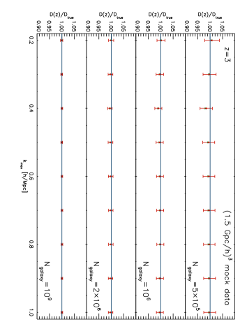
To simulate the mock data, we take a simplified approach: we take our best-fitting power spectrum at $z=3$, i.e., Eq. (2) fit to the power spectrum of MPA halos in the Millennium Simulation at $z=3$, and add random Gaussian noise to it with the standard deviation given by Eq. (7). To compute the standard deviation we need to specify the survey volume, which determines the fundamental wavenumber, $\Delta k$, as $\Delta k=2\pi/V_{survey}^{1/3}$. We use the volume that would be surveyed by the HETDEX survey (Hill et al., 2004), $V_{survey}=(1.5~{}\mathrm{Gpc}/h)^{3}$, which is 27 times as large as the volume of the Millennium Simulation. We then vary the number of galaxies, $N_{galaxy}$, which determines the shot noise as $P_{shot}=1/n=V_{survey}/N_{galaxy}$. We have generated only one realization, and repeated the same analysis as before to extract $D_{A}$ from the mock HETDEX data.

In Figure 20 we show $D/D_{true}$ as a function of $k_{max}$ and $N_{g}$. For $N_{galaxy}=10^{9}$, which gives the same number density as the Millennium Simulation, the projected error on $D$ is 0.3%, or 8 times better than the original result presented in Figure 16. Since the volume is 27 times bigger, the statistics alone would reduce the error by a factor of about 5.

The other factor of about 1.5 comes from the fact that the variance of the distance scale estimated from the Millennium Simulation lies on the tail of the distribution of the variance of the distance scale, (See, appendix C) while the error estimated from the HETDEX volume mock is close to the peak of PDF of the variance.

However, real surveys will not get as high the number density as the Millennium Simulation. For example, the HETDEX survey will detect about one million Ly$\alpha$ emitting galaxies, i.e., $N_{galaxy}=10^{6}$. In Figure 20 we show that the errors on $D$ increase from 0.3% for $N_{galaxy}=10^{9}$ to 1%, 1.5%, and 3% for $N_{galaxy}=2\times 10^{6}$, $10^{6}$, and $2\times 10^{5}$, respectively.

Finally, we note that these forecasts are not yet final, as we have not included the effect of non-linear redshift space distortion. Also, eventually one needs to repeat this analysis using the “super Millennium Simulation” with a bigger volume.

6. Discussion and Conclusions

Two main new results that we have presented in this paper are:

• The 3rd-order PT galaxy power spectrum given by Eq. (2), which is based upon the assumption that the number density of galaxies at a given location is a local function of the underlying matter density at the same location (Fry & Gaztanaga, 1993) plus stochastic noise (McDonald, 2006), fits the halo as well as galaxy power spectra estimated from the Millennium Simulation at high redshifts, $1\leq z\leq 6$, up to the maximum wavenumber, $k_{max}$, that has been determined from the matter power spectrum.

• When 3 galaxy bias parameters, $\tilde{b}_{1}$, $\tilde{b}_{2}$, and $P_{0}$, are marginalized over, the 3rd-order PT galaxy power spectrum fit to the Millennium Simulation yields the correct (unbiased) distance scale to within the statistical error of the simulation, $\sim 3\%$.

These results suggest that the 3rd-order PT provides us with a practical means to extract the cosmological information from the observed galaxy power spectra at high redshifts, i.e., $z>1$, accurately.

We would like to emphasize that our approach does not require simulations to calibrate the model. The 3rd-order PT is based upon the solid physical framework, and the only assumption made for the galaxy formation is that it is a local process, at least on the scales where the 3rd-order PT is valid, i.e., $k<k_{max}$. The only serious drawback so far is that the 3rd-order PT breaks down at low redshifts, and thus it cannot be applied to the current generation of survey data such as 2dFGRS and SDSS. However, the planned future high-$z$ surveys would benefit immensely from the PT approach.

The practical application of our approach may proceed as follows:

• Measure the galaxy power spectra at various redshifts. When we have $N$ redshift bins, the number of bias parameters is $3N$, as the bias parameters evolve with $z$.

• Calculate $k_{max}(z)$ from the condition, $\Delta_{m}^{2}(k_{max},z)=0.4$, where $\Delta_{m}^{2}(k,z)=k^{3}P_{\delta\delta}(k,z)/(2\pi^{2})$ is computed from the fiducial cosmology, e.g., the WMAP 5-year best-fitting parameters. The results should not be sensitive to the exact values of $k_{max}(z)$.

• Fit Eq. (2) to the observed galaxy spectra up to $k_{max}(z)$ at all $z$ simultaneously for extracting the cosmological parameters.

In addition to this, we should be able to improve upon the accuracy of parameter determinations by including the bispectrum as well, as the bispectrum basically fixes $\tilde{b}_{1}$ and $\tilde{b}_{2}$ (Sefusatti & Komatsu, 2007). Therefore, the step (3) may be replaced by

• Fit Eq. (2) to the observed galaxy spectra up to $k_{max}(z)$, and fit the PT bispectrum to the observed galaxy bispectra up to the same $k_{max}(z)$, at all $z$ simultaneously for extracting the cosmological parameters.

We are currently performing a joint analysis of the galaxy power spectra and bispectra on the Millennium Simulation. The results will be reported elsewhere.

There are limitations in our present study, however. First, a relatively small volume of the Millennium Simulation does not allow us to make a precision test of the 3rd-order PT. Also, this limitation does not allow us to study constraints on more than one cosmological parameter. We have picked $D$ as the representative example because this parameter seems the most interesting one in light of the future surveys whose primary goal is to constrain the properties of dark energy. In the future we must use larger simulations to show convincingly that the bias in cosmological parameters is much lower than 1% level. Second, we have found that, due to the limited statistics of a small volume and the smaller $k_{max}$ due to stronger non-linearities, the bias parameters are not determined very well from the galaxy power spectra alone at $z\leq 3$. This issue should disappear by including the bispectrum in the joint analysis. Last and foremost, our study has been restricted to the real space power spectra: we have not addressed the non-linearities in redshift space distortion. This is a subject of the future study.

Appendix A Error on power spectrum

Besides the normalization, an estimator for the power spectrum may be written as

$$P_{obs}(k)=\frac{1}{N_{k}}\sum_{i=1}^{N_{k}}|\delta(\mathbf{k}_{i})|^{2}\Biggl{|}_{|\mathbf{k}_{i}-k|\leq\Delta k}$$ (A1)

where $\delta(\mathbf{k}_{i})$ is a Fourier transform of the density field in position space, $\Delta k$ is the fundamental wavenumber of either survey volume or simulation box, and $N_{k}$ is the number of independent $k$-modes available per bin. This estimator is unbiased because

$$\langle P_{obs}(k)\rangle=\frac{1}{N_{k}}\sum_{i=1}^{N_{k}}\langle|\delta(\mathbf{k}_{i})|^{2}\rangle\Biggl{|}_{|\mathbf{k}_{i}-k|\leq\Delta k}=\langle|\delta(k)|^{2}\rangle=P(k),$$ (A2)

where $P(k)$ is the underlying power spectrum. The variance of this estimator is given by

$$\left\langle\left(\frac{P_{obs}(k)-P(k)}{P(k)}\right)^{2}\right\rangle=1-2\frac{\langle P_{obs}\rangle}{P(k)}+\frac{1}{N_{k}^{2}P(k)^{2}}\sum_{i=1}^{N_{k}}\sum_{j=1}^{N_{k}}\langle\delta^{*}(\mathbf{k}_{i})\delta(\mathbf{k}_{i})\delta^{*}(\mathbf{k}_{j})\delta(\mathbf{k}_{j})\rangle.$$ (A3)

Assuming that the density field is a Gaussian random variable with its variance given by $P(k)$, i.e.,

$$\langle\delta_{i}^{*}\delta_{j}\rangle=P(k)\delta_{ij},$$ (A4)

we use Wick’s theorem for evaluating the last double summation:

$$\sum_{i=1}^{N_{k}}\sum_{j=1}^{N_{k}}\langle\delta^{*}_{i}\delta_{i}\delta^{*}_{j}\delta_{j}\rangle = \sum_{i=1}^{N_{k}}\sum_{j=1}^{N_{k}}\left[\langle\delta^{*}_{i}\delta_{i}\rangle\langle\delta^{*}_{j}\delta_{j}\rangle+\langle\delta^{*}_{i}\delta_{j}\rangle\langle\delta^{*}_{j}\delta_{i}\rangle+\langle\delta^{*}_{i}\delta^{*}_{j}\rangle\langle\delta_{i}\delta_{j}\rangle\right]$$ (A5)

$$= N_{k}^{2}[P(k)]^{2}+N_{k}[P(k)]^{2}.$$

Therefore, the variance is given by

$$\left\langle\left[P_{obs}(k)-P(k)\right]^{2}\right\rangle=\frac{[P(k)]^{2}}{N_{k}},$$ (A6)

and the standard deviation is given by

$$\sigma_{P(k)}\equiv\left\langle\left[P_{obs}(k)-P(k)\right]^{2}\right\rangle^{1/2}=\sqrt{\frac{1}{N_{k}}}P(k).$$ (A7)

Note that this formula is valid only when $\delta$ is a Gaussian random field. When $\delta$ is non-Gaussian due to, e.g., non-linear evolution, primordial non-Gaussianity, non-linear bias, etc., we must add the connected four-point function to Eq. (A5). See also Takahashi et al. (2008) for the study of finite box size effects on the four-point function.

How do we calculate $N_{k}$? As the Fourier transformation of a real-valued field has symmetry given by $\delta^{*}(\mathbf{k})=\delta(-\mathbf{k})$, the number of independent $k$-modes is exactly a half of the number of modes available in a spherical shell at a given $k$. We find

$$N_{k}=\frac{1}{2}\frac{4\pi k^{2}\delta k}{(\delta k)^{3}}=2\pi\left(\frac{k}{\delta k}\right)^{2},$$ (A8)

where $\delta k$ is the fundamental wavenumber given by $\delta k=2\pi/L$, where $L$ is the survey size or simulation box size.

In the literature one may often find a different formula such as

$$\sigma_{P(k)}^{literature}=\sqrt{\frac{2}{N^{literature}_{k}}}P(k).$$ (A9)

Here, there is an extra factor of $\sqrt{2}$, as $N^{literature}_{k}$ is the number of modes available in a spherical shell at a given $k$, without symmetry, $\delta^{*}(\mathbf{k})=\delta(-\mathbf{k})$, taken into account, i.e., $N^{literature}_{k}=2N_{k}$. Both formulas give the same results, provided that we understand what we mean by $N_{k}$ in these formulas.

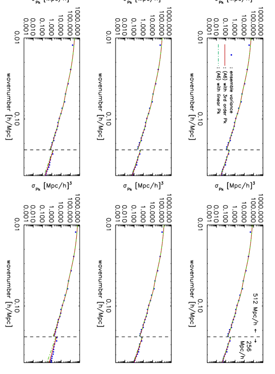
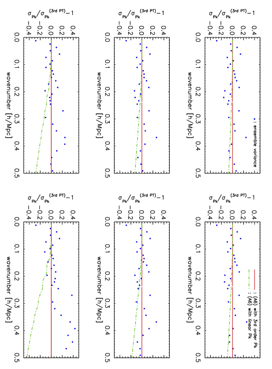
We have tested the formula Eq. (A7) by comparing it to the standard deviation estimated the ensemble of dark matter simulations used in Paper I. (See Paper I for details of the simulations.) Figure 21 and 22 show the result of this comparison. The formula Eq. (A7) and the simulation data agree well.

Figure 21.— Standard deviation of the matter power spectrum: analytical versus simulations. The symbols show the standard deviations directly measured from 120 independent $N$-body simulations whose box sizes are $L=512~{}\mathrm{Mpc}/h$ (60 realizations for $k<0.24h/\mathrm{Mpc}$) and $L=256~{}\mathrm{Mpc}/h$ (60 realizations for $0.24<k<0.5h/\mathrm{Mpc}$) . Each simulation contains $256^{3}$ particles. The solid and dot-dashed lines show the analytical formula (Eq. (A7)) with the 3rd-order PT non-linear $P(k)$ and the linear $P(k)$, respectively. Note that the graph is discontinuous at $k=0.24h/\mathrm{Mpc}$ because the number of $k$ modes, $N_{k}$, for a given wavenumber $k$ is different for different box sizes.

Figure 22.— Residuals. We divide both analytical estimation and simulation results by the analytical formula (Eq. (A7)) with the 3rd-order PT nonlinear $P(k)$.

Appendix B Analytical marginalization of the likelihood function over $\tilde{b}_{1}^{2}$ and $P_{0}$

In this appendix we derive the analytical formulas for the likelihood function marginalized over $\tilde{b}_{1}^{2}$ and $P_{0}$.

The likelihood function, Eq. (6), is given by

$$\mathcal{L}(\tilde{b}_{1},\tilde{b}_{2},P_{0},\theta_{n})=\left(\prod_{i}\frac{1}{\sqrt{2\pi\sigma_{Pi}^{2}}}\right)\exp\left[-\sum_{i}\frac{\left(P_{obs,i}-\tilde{b}_{1}^{2}(P_{\delta\delta,i}+\tilde{b}_{2}P_{b2,i}+\tilde{b}_{2}^{2}P_{b22,i})-P_{0}\right)^{2}}{2\sigma_{Pi}^{2}}\right],$$ (B1)

where $\theta_{n}$ are the cosmological parameters that do not depend on any of the bias parameters. The subscript $i$ denotes bins, $k_{i}$.

Integrating the likelihood function over $P_{0}$, we find

$$\mathcal{L}(\tilde{b}_{1},\tilde{b}_{2},\theta_{n}) = \int_{-\infty}^{\infty}dP_{0}\mathcal{L}(\tilde{b}_{1},\tilde{b}_{2},P_{0},\theta_{n})$$ (B2)

$$= \mathcal{N}\sqrt{\frac{2\pi}{\sum_{i}w_{i}}}\exp\left[-\frac{1}{2}\frac{\sum_{i>j}w_{i}w_{j}(a_{j}-a_{i})^{2}}{\sum_{i}w_{i}}\right],$$

where we have defined new variables

$$\mathcal{N} \equiv \prod_{i}\frac{1}{\sqrt{2\pi\sigma_{Pi}^{2}}}$$ (B3)

$$a_{i} \equiv P_{obs,i}-\tilde{b}_{1}^{2}(P_{\delta\delta,i}+\tilde{b}_{2}P_{b2,i}+\tilde{b}_{2}^{2}P_{b22,i})$$ (B4)

$$w_{i} \equiv \frac{1}{\sigma_{Pi}^{2}}.$$ (B5)

We then integrate this function over $\tilde{b}_{1}^{2}$. Introducing new variables given by

$$\bar{\mathcal{N}} \equiv \mathcal{N}\sqrt{\frac{2\pi}{\sum_{i}w_{i}}},$$ (B6)

$$P_{th,i} \equiv P_{\delta\delta,i}+\tilde{b}_{2}P_{b2,i}+\tilde{b}_{2}^{2}P_{b22,i},$$ (B7)

and $a_{i}=P_{obs,i}-\tilde{b}_{1}^{2}P_{th,i}$, we rewrite Eq. (B2) as

$$\mathcal{L}(\tilde{b}_{1},\tilde{b}_{2},\theta_{n}) = \bar{\mathcal{N}}\exp\left[-\frac{1}{2}\frac{\sum_{i>j}w_{i}w_{j}\left\{(P_{th,i}-P_{th,j})\tilde{b}_{1}^{2}-(P_{obs,i}-P_{obs,j})\right\}^{2}}{\sum_{i}w_{i}}\right]$$ (B8)

$$= \bar{\mathcal{N}}\exp\left[-\frac{1}{2}\left(A\tilde{b}_{1}^{4}-2B\tilde{b}_{1}^{2}+C\right)\right],$$

where

$$A \equiv \frac{\sum_{i>j}w_{i}w_{j}(P_{th,i}-P_{th,j})^{2}}{\sum_{i}w_{i}}$$ (B9)

$$B \equiv \frac{\sum_{i>j}w_{i}w_{j}(P_{th,i}-P_{th,j})(P_{obs,i}-P_{obs,j})}{\sum_{i}w_{i}}$$ (B10)

$$C \equiv \frac{\sum_{i>j}w_{i}w_{j}(P_{obs,i}-P_{obs,j})^{2}}{\sum_{i}w_{i}}.$$ (B11)

Assuming a flat prior on $\tilde{b}_{1}^{2}$, we integrate the likelihood function to find the desired result:

$$\mathcal{L}(\tilde{b}_{2},\theta_{n}) = \bar{\mathcal{N}}\int_{0}^{\infty}\exp\left[-\frac{1}{2}\left(A\tilde{b}_{1}^{4}-2B\tilde{b}_{1}^{2}+C\right)\right]d(\tilde{b}_{1}^{2})$$ (B12)

$$= \bar{\mathcal{N}}\exp\left[\frac{B^{2}-AC}{2A}\right]\sqrt{\frac{\pi}{2A}}\left\{1+\rm{erf}\left(\frac{B}{\sqrt{2A}}\right)\right\}.$$

Note that the convergence of the likelihood function is ensured by Cauchy’s inequality, $B^{2}-AC<0$.

Appendix C distribution of errors on the distance scale

We find that the error on $D$ extracted from the halo power spectrum of Millennium Simulation is about $2.17\%$ for $k_{max}=1.5~{}h/\mathrm{Mpc}$ at $z=6$. (See Figure 16.) On the other hand, the error on $D$ calculated from the Fisher information matrix is $1.57\%$ Are they consistent?

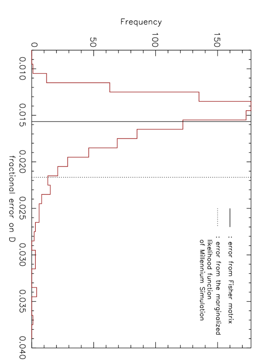
In order to test whether it is possible to get the error on $D$ far from the value derived from the Fisher matrix, we generate $1000$ realizations of mock power spectra with the best-fitting bias parameters for halo with $k_{max}=1.5~{}h/\mathrm{Mpc}$ at $z=6$. Then, we calculate the best-fitting value of $D$ as well as the 1-$\sigma$ ($68.27\%$ CL) range from the one-dimensional marginalized likelihood function of $D$ for each realization.

We find that the mean 1-$\sigma$ error on $D$ calculated from these realizations is $1.66\%$, and their standard deviation is $0.43\%$. Figure 23 shows the distribution of the fractional 1-$\sigma$ error on $D$ compared with $D_{true}$. While the error derived from the Fisher matrix is close to the mean, the error calculated from the Millennium Simulation is on the tail of the distribution. The probability of having an error on $D$ greater than that from the Millennium Simulation is about $6\%$, which is acceptable.

Figure 23.— Histogram for the 1-$\sigma$ errors on $D$ calculated from $1000$ Monte Carlo realizations generated with the best-fitting bias parameters of halo power spectrum of Millennium Simulation with $k_{max}=1.5~{}h/\mathrm{Mpc}$ at $z=6$. The error derived from the Fisher matrix is close to the mean, while the error from the marginalized one-dimensional likelihood function of Millennium Simulation is on the tail of the distribution. The probability of having an error on $D$ greater than that from the Millennium Simulation is about $6\%$.

References

- Angulo et al. (2008) Angulo, R. E., Baugh, C. M., Frenk, C. S., & Lacey, C. G. 2008, MNRAS, 383, 755
- Bennett et al. (2003) Bennett, C. L., et al. 2003, ApJ, 583, 1
- Benson et al. (2003) Benson, A. J., Bower, R. G., Frenk, C. S., Lacey, C. G., Baugh, C. M., & Cole, S. 2003, ApJ, 599, 38
- Bernardeau et al. (2002) Bernardeau, F., Colombi, S., Gaztañaga, E., & Scoccimarro, R. 2002, Phys. Rep., 367, 1
- Bond et al. (1991) Bond, J. R., Efstathiou, G., Lubin, P. M., & Meinhold, P. R. 1991, Phys. Rev. Lett., 66, 2179
- Bower et al. (2006) Bower, R. G., Benson, A. J., Malbon, R., Helly, J. C., Frenk, C. S., Baugh, C. M., Cole, S., & Lacey, C. G. 2006, MNRAS, 370, 645
- Chabrier (2003) Chabrier, G. 2003, PASP, 115,763
- Cole et al. (2000) Cole, S., Lacey, C. G., Baugh, C. M., & Frenk, C. S. 2000, MNRAS, 319, 168
- Cole et al. (2005) Cole, S., et al. 2005, MNRAS, 362, 505
- Cooray & Sheth (2002) Cooray, A. & Sheth, R. 2002, Phys. Rep., 372, 1
- Copeland et al. (2006) Copeland, E. J., Sami, M., & Tsujikawa, S. 2006, Int. J. Mod. Phys., D15, 1753
- Crocce et al. (2006) Crocce, M., Pueblas, S., & Scoccimarro, R. 2006, MNRAS, 373, 369
- Crocce & Scoccimarro (2008) Crocce, M. & Scoccimarro, R. 2008, Phys. Rev. D, 77, 023533
- Croton et al. (2006) Croton, D. J., et al. 2006, MNRAS, 365, 11
- De Lucia & Blaizot (2007) De Lucia, G. & Blaizot, J. 2007, MNRAS, 375, 2
- Dunkley et al. (2008) Dunkley, J., et al. 2008, ArXiv e-prints, 803
- Eisenstein & Hu (1998) Eisenstein, D. J. & Hu, W. 1998, ApJ, 496, 605
- Eisenstein et al. (2007) Eisenstein, D. J., Seo, H.-J., & White, M. 2007, ApJ, 664, 660
- Eisenstein et al. (2005) Eisenstein, D. J., et al. 2005, ApJ, 633, 560
- Fry (1996) Fry, J. N. 1996, ApJ, 461, L65+
- Fry & Gaztanaga (1993) Fry, J. N. & Gaztanaga, E. 1993, ApJ, 413, 447
- Glazebrook et al. (2005) Glazebrook, K., Eisenstein, D., Dey, A., Nichol, B., & The WFMOS Feasibility Study Dark Energy Team. 2005, ArXiv Astrophysics e-prints
- Heavens et al. (1998) Heavens, A. F., Matarrese, S., & Verde, L. 1998, MNRAS, 301, 797
- Heitmann et al. (2007) Heitmann, K., et al. 2007, ArXiv e-prints, 706
- Hill et al. (2004) Hill, G. J., Gebhardt, K., Komatsu, E., & MacQueen, P. J. 2004, in American Institute of Physics Conference Series, Vol. 743, The New Cosmology: Conference on Strings and Cosmology, ed. R. E. Allen, D. V. Nanopoulos, & C. N. Pope, 224–233
- Hinshaw et al. (2003) Hinshaw, G., et al. 2003, ApJS, 148, 135
- Hinshaw et al. (2007) —. 2007, ApJS, 170, 288
- Hinshaw et al. (2008) —. 2008, ArXiv e-prints, 803
- Huff et al. (2007) Huff, E., Schulz, A. E., White, M., Schlegel, D. J., & Warren, M. S. 2007, Astroparticle Physics, 26, 351
- Jain & Bertschinger (1994) Jain, B. & Bertschinger, E. 1994, ApJ, 431, 495
- Jeong & Komatsu (2006) Jeong, D. & Komatsu, E. 2006, ApJ, 651, 619
- Jing (2005) Jing, Y. P. 2005, ApJ, 620, 559
- Kaiser (1984) Kaiser, N. 1984, ApJ, 284, L9
- Kennicutt (1983) Kennicutt, R. C., Jr. 1983, ApJ, 272, 54
- Kogut et al. (2003) Kogut, A., et al. 2003, ApJS, 148, 161
- Komatsu et al. (2008) Komatsu, E., et al. 2008, ArXiv e-prints, 803
- Matarrese & Pietroni (2007) Matarrese, S. & Pietroni, M. 2007, Journal of Cosmology and Astro-Particle Physics, 6, 26
- Matarrese et al. (1997) Matarrese, S., Verde, L., & Heavens, A. F. 1997, MNRAS, 290, 651
- Matsubara (2008) Matsubara, T. 2008, Phys. Rev. D, 77, 063530
- McDonald (2006) McDonald, P. 2006, Phys. Rev. D, 74, 103512
- McDonald (2007) —. 2007, Phys. Rev. D, 75, 043514
- Meiksin et al. (1999) Meiksin, A., White, M., & Peacock, J. A. 1999, MNRAS, 304, 851
- Nishimichi et al. (2007) Nishimichi, T., et al. 2007, PASJ, 59, 1049
- Nolta et al. (2008) Nolta, M. R. et al. 2008, ApJS
- Page et al. (2007) Page, L., et al. 2007, ApJS, 170, 335
- Peebles (1993) Peebles, P. J. E. 1993, Principles of Physical Cosmology (Princeton, NJ: Princeton University Press)
- Percival et al. (2007) Percival, W. J., Cole, S., Eisenstein, D. J., Nichol, R. C., Peacock, J. A., Pope, A. C., & Szalay, A. S. 2007, MNRAS, 381, 1053
- Perlmutter et al. (1999) Perlmutter, S., et al. 1999, ApJ, 517, 565
- Riess et al. (1998) Riess, A. G., et al. 1998, AJ, 116, 1009
- Sanchez et al. (2008) Sanchez, A. G., Baugh, C. M., & Angulo, R. 2008, ArXiv e-prints, 804
- Scoccimarro (1998) Scoccimarro, R. 1998, MNRAS, 299, 1097
- Scoccimarro et al. (2001) Scoccimarro, R., Feldman, H. A., Fry, J. N., & Frieman, J. A. 2001, ApJ, 546, 652
- Sefusatti et al. (2006) Sefusatti, E., Crocce, M., Pueblas, S., & Scoccimarro, R. 2006, Phys. Rev. D, 74, 023522
- Sefusatti & Komatsu (2007) Sefusatti, E. & Komatsu, E. 2007, Phys. Rev. D, 76, 083004
- Seljak (2000) Seljak, U. 2000, MNRAS, 318, 203
- Seo & Eisenstein (2003) Seo, H.-J. & Eisenstein, D. J. 2003, ApJ, 598, 720
- Seo & Eisenstein (2005) Seo, H.-J. & Eisenstein, D. J. 2005, Astrophys. J., 633, 575
- Seo et al. (2008) Seo, H.-J., Siegel, E. R., Eisenstein, D. J., & White, M. 2008, ArXiv e-prints, 805
- Sheth & Tormen (1999) Sheth, R. K. & Tormen, G. 1999, MNRAS, 308, 119
- Shoji et al. (2008) Shoji, M., Jeong, D., & Komatsu, E. 2008, To be submitted
- Smith et al. (2007) Smith, R. E., Scoccimarro, R., & Sheth, R. K. 2007, Phys. Rev. D, 75, 063512
- Smith et al. (2008) —. 2008, Phys. Rev. D, 77, 043525
- Spergel et al. (2003) Spergel, D. N., et al. 2003, ApJS, 148, 175
- Spergel et al. (2007) —. 2007, ApJS, 170, 377
- Springel (2005) Springel, V. 2005, MNRAS, 364, 1105
- Springel et al. (2001) Springel, V., Yoshida, N., & White, S. D. M. 2001, New Astronomy, 6, 79
- Springel et al. (2005) Springel, V., et al. 2005, Nature, 435, 629
- Takada et al. (2006) Takada, M., Komatsu, E., & Futamase, T. 2006, Phys. Rev. D, 73, 083520
- Takahashi et al. (2008) Takahashi, R., et al. 2008, ArXiv e-prints, 802
- Taruya & Hiramatsu (2008) Taruya, A. & Hiramatsu, T. 2008, ApJ, 674, 617
- Tegmark (1997) Tegmark, M. 1997, Physical Review Letters, 79, 3806
- Tegmark & Peebles (1998) Tegmark, M. & Peebles, P. J. E. 1998, ApJ, 500, L79+
- Tegmark et al. (2006) Tegmark, M., et al. 2006, Phys. Rev. D, 74, 123507
- Valageas (2007) Valageas, P. 2007, A&A, 465, 725
- Weinberg (2008) Weinberg, S. 2008, Cosmology (Oxford, UK: Oxford University Press)
- Yoshikawa et al. (2001) Yoshikawa, K., Taruya, A., Jing, Y. P., & Suto, Y. 2001, ApJ, 558, 520