Interface Tension of Bose-Einstein Condensates

Abstract

Motivated by recent observations of phase-segregated binary Bose-Einstein condensates, we propose a method to calculate the excess energy due to the interface tension of a trapped configuration. By this method one should be able to numerically reproduce the experimental data by means of a simple Thomas-Fermi approximation, combined with interface excess terms and the Laplace equation. Using the Gross-Pitaevskii theory, we find expressions for the interface excesses which are accurate in a very broad range of the interspecies and intraspecies interaction parameters. We also present finite-temperature corrections to the interface tension which, aside from the regime of weak segregation, turn out to be small.

I Introduction

Soon after the first experimental realization of Bose-Einstein condensation (BEC) in dilute gases, binary BEC mixtures were realized modugno ; miesner ; myatt ; stamper ; hall ; matthews ; stenger ; thalhammer ; papp ; papp2 . These experiments precipitated a strong theoretical interest, the origin of which is the fact that the multicomponent BEC is not a trivial extension of the single-component BEC ho ; graham ; pu ; esry ; esry2 ; ohberg ; alexandrov ; timmermans ; law ; bashkin ; burke ; busch ; riboli ; jezek ; mazets ; ao ; ao2 ; svidzinsky ; barankov ; chui . Indeed, novel and fundamentally different physics arise on both microscopic and macroscopic levels. Phenomena studied for binary mixtures so far include the quantum tunnelling of spin domains stamper ; miesner , spin-relaxation processes miesner , vortex configurations matthews , formation of Feshbach molecules papp and collective oscillations modugno . Experiments with phase-segregated BEC mixtures were established already in 1998 stenger ; hall ; this triggered many theorists to focus on the observed weakly-segregated phases whereby the importance of the interface physics was highlighted several times ao ; ao2 ; chui ; alexandrov ; svidzinsky ; mazets ; timmermans ; barankov ; riboli ; jezek .

Also surfaces of single-component BEC gases have gained much attention. Studies are performed on vortices, surface modes and tunnelling phenomena at the border of a trapped single-component BEC lundh ; dalfovo ; khawaja ; fetter2 and on BEC diffraction and van der Waals forces using an optical mirror or evanescent-wave prism colombe ; rychtarik ; landragin . Moreover a combination of the interface physics of binary BEC gases and the surface physics near hard walls led to the theoretical prediction of anomalous wetting phase transitions indekeu .

The clearest observation so far of phase segregation of BEC mixtures was reported by Papp et al. (see Ref. papp2, ) who used a mixture of ⁸⁵Rb and ⁸⁷Rb particles. By changing the particle numbers of both species and the intraspecies interactions of the ⁸⁵Rb particles by use of a Feshbach resonance, many topologically distinct states were encountered. In the phase-segregated regime most trap configurations contained BEC droplets. Papp et al. stated that a detailed theoretical understanding of the observed droplet formation is lacking. As an essential first step towards this understanding we present here expressions for the interface tension. Moreover, we also formulate a method by which all trap configurations can be straightforwardly studied by the use of a local density approximation or Thomas-Fermi approximation. At first sight, numerically reproducing the experimentally observed (meta)stable states requires solving the coupled Gross-Pitaevskii (GP) equations for the full three-dimensional system; in such case, a high accuracy is indispensable to capture the important energy contributions near the two-phase boundaries which strongly affect the ground state topology.

In this work, we argue that it is not necessary to solve the full GP system in order to recover numerically the experimental configurations; instead, one can find the ground state, that is, minimize the total energy of the trapped cloud, by use of the Thomas-Fermi approximation and the expressions for the interface tension which we provide here. This allows an omission of the quantum pressure term which strongly complicates the numerical work. The analytical calculation of the interface tension is nontrivial as it involves solving the binary GP equations (i.e. two coupled nonlinear second-order differential equations). Estimates and analytical expressions were already given in Refs. timmermans, -barankov, and were relevant to the early experiments on weakly-segregated mixtures but irrelevant to the interfaces as observed in Ref. papp2, since there segregation is not weak. By developing expansions, we succeed in obtaining analytical expressions for the interface tension which are accurate for almost all parameter regimes.

As a main result we find that, even though the interface tension is not constant throughout the trap, the total excess energy $\Omega_{\mathcal{A}}$ can be reduced to a simple integral of the trapping potential along the interface area $\mathcal{A}$:

$$\Omega_{\mathcal{A}} =\frac{\sqrt{2m_{{}_{1}}}}{4\pi\hslash a_{{}_{11}}}\mathcal{F}(\xi_{{}_{2}}/\xi_{{}_{1}},K)\int_{{}_{\mathcal{A}}}\text{d}\mathbf{r}\,[\mu_{{}_{1}}-U_{{}_{1}}(\mathbf{r})]^{3/2},$$ (1)

where $a_{{}_{11}}$, $m_{{}_{1}}$, $\mu_{{}_{1}}$ and $U_{{}_{1}}$ are the intraspecies scattering length, the particle mass, the chemical potential and the applied trapping potential of phase $1$. The parameters $K$ and $\xi_{{}_{2}}/\xi_{{}_{1}}$ can be expressed in terms of the atomic masses and the interspecies and intraspecies scattering lengths:

$$K=\frac{m_{{}_{1}}+m_{{}_{2}}}{2\sqrt{m_{{}_{1}}m_{{}_{2}}}}\frac{a_{{}_{12}}}{\sqrt{a_{{}_{11}}a_{{}_{22}}}}\text{ and }\xi_{{}_{2}}/\xi_{{}_{1}}=\sqrt[4]{\frac{m_{{}_{1}}a_{{}_{11}}}{m_{{}_{2}}a_{{}_{22}}}}.$$ (2)

For a broad range of values of $\xi_{{}_{2}}/\xi_{{}_{1}}$ and $K$, the function $\mathcal{F}$ can be written as:

$$\mathcal{F}(\xi_{{}_{2}}/\xi_{{}_{1}},K)=\frac{\sqrt{2}}{3}(1+\xi_{{}_{2}}/\xi_{{}_{1}})-\frac{0.514\sqrt{\xi_{{}_{2}}/\xi_{{}_{1}}}}{K^{1/4}}$$ (3)

$$-\sqrt{\xi_{{}_{2}}/\xi_{{}_{1}}}(\xi_{{}_{2}}/\xi_{{}_{1}}+\xi_{{}_{1}}/\xi_{{}_{2}})\left(\frac{0.055}{K^{3/4}}+\frac{0.067}{K^{5/4}}\right)+\ldots.$$

This work is structured as follows. We start off in Sect. II by introducing the GP formalism for binary BECs. After defining the excess energy in a homogeneous and in a trapped system in Sect. III, we find analytical expressions for the interface tension in Sect. IV. We estimate the finite-temperature corrections to the interface tension in Sect. V. In Sect. VI we discuss the experimental relevance of our findings.

II Binary BEC System

Equilibrium states of a mixture of two dilute BEC gases with order parameters $\Psi_{{}_{1}}$ and $\Psi_{{}_{2}}$ and chemical potentials $\mu_{{}_{1}}$ and $\mu_{{}_{2}}$, are well modelled using the grand potential:

$$\Omega(\mu_{{}_{1}},\mu_{{}_{2}},V)= \sum_{i=1,2}\left(\int_{{}_{V}}{\text{d}\mathbf{r}\,\Psi_{{}_{i}}^{*}(\mathbf{r})\left[-\frac{\hslash^{2}}{2m_{{}_{i}}}\boldsymbol{\nabla}^{2}-\mu_{{}_{i}}+U_{{}_{i}}(\mathbf{r})\right]\Psi_{{}_{i}}(\mathbf{r})}+\frac{G_{{}_{ii}}}{2}|\Psi_{{}_{i}}(\mathbf{r})|^{4}\right)+G_{{}_{12}}\int_{{}_{V}}{\text{d}\mathbf{r}\,|\Psi_{{}_{1}}(\mathbf{r})|^{2}|\Psi_{{}_{2}}(\mathbf{r})|^{2}},$$ (4)

where $G_{{}_{ij}}=2\pi\hslash^{2}a_{{}_{ij}}(m_{{}_{i}}^{-1}+m_{{}_{j}}^{-1})$ are the coupling constants and $a_{{}_{ij}}$ are the s-wave scattering lengths (henceforth $i=1,\,2$). In view of the derivation of the interface tension, we continue here by assuming vanishing external potentials $U_{{}_{1}}=U_{{}_{2}}=0$; we reintroduce the external potentials when discussing the surface excess of a trapped system. In the absence of particle flow one can choose the order parameters to be real valued such that the equilibrium pressures for the pure states are:

$$P_{{}_{i}}=\frac{\mu^{2}_{{}_{i}}}{2G_{{}_{ii}}}.$$ (5)

In order to study phase-segregated states of the two coexisting condensates, we introduce the parameter

$$K\equiv\frac{G_{{}_{12}}}{\sqrt{G_{{}_{11}}G_{{}_{22}}}},$$ (6)

which quantifies the interspecies couplings relative to the average of the intraspecies couplings. It is well-known that when $K$ exceeds one, the species become immiscible and only pure phases can exist ao while phase mixing occurs when $K<1$. Along the two-phase interface, coexistence is ensured by the condition:

$$\frac{\mu_{{}_{1}}^{2}}{2G_{{}_{11}}}=\frac{\mu_{{}_{2}}^{2}}{2G_{{}_{22}}}.$$ (7)

Henceforth we assume that $K>1$ and that the chemical potentials are such that the bulk pressures are $P_{{}_{1}}=P_{{}_{2}}\equiv P$. For calculational convenience, we further rescale the order parameters $\Psi_{{}_{1}}$ and $\Psi_{{}_{2}}$ and define the dimensionless wave functions $\psi_{{}_{1}}$ and $\psi_{{}_{2}}$:

$$\Psi_{{}_{i}}\equiv\psi_{{}_{i}}\sqrt{\frac{\mu_{{}_{i}}}{G_{{}_{ii}}}}.$$ (8a)

The quantum nature of the system results in a zero-point motion; this determines the typical length scale for density modulations at boundaries, impurities, vortices or solitons. For the pure phases, the resultant length is the healing length $\xi_{{}_{i}}$ which is defined as:

$$\xi_{{}_{i}}\equiv\frac{\hslash}{\sqrt{2m_{{}_{i}}\mu_{{}_{i}}}}.$$ (9)

Without loss of generality, we choose the phases such that $\xi_{{}_{2}}/\xi_{{}_{1}}\leq 1$. As coexistence must occur along the interface, $K$ and $\xi_{{}_{2}}/\xi_{{}_{1}}$ can be expressed in terms of the atomic masses and the scattering lengths as given in Eq. (2). Finally, after rescaling the space coordinate to the dimensionless variable $\widetilde{\mathbf{r}}\equiv\mathbf{r}/\xi_{{}_{1}}$, the reduced time-independent Gross-Pitaevskii (GP) Eqs. are pita ; pethick :

$$\boldsymbol{\nabla}^{2}\psi_{{}_{1}}= -\psi_{{}_{1}}+\psi_{{}_{1}}^{3}+K\psi_{{}_{1}}\psi_{{}_{2}}^{2},$$ (10a)

$$[\xi_{{}_{2}}/\xi_{{}_{1}}]^{2}\boldsymbol{\nabla}^{2}\psi_{{}_{2}}= -\psi_{{}_{2}}+\psi_{{}_{2}}^{3}+K\psi_{{}_{2}}\psi_{{}_{1}}^{2}.$$ (10b)

Having established the equations of motion, we continue now by defining the interface tension.

III Definition of Interface Tension and interface Excess

In order to calculate the interface tension, consider two BEC components in an infinitely large system with translational symmetry in the $x$-$y$ direction. The presence of phase $1$ at $z\rightarrow\infty$ and of phase $2$ at $z\rightarrow-\infty$ imply the following boundary conditions:

$$\psi_{{}_{1}}(z =-\infty)=\psi_{{}_{2}}(z=\infty)=0,$$ (11a)

$$\psi_{{}_{1}}(z =\infty)=\psi_{{}_{2}}(z=-\infty)=1.$$ (11b)

Under these conditions, the first integral of the reduced GP Eqs. (10a) and (10b) is:

$$\dot{\psi}_{{}_{1}}^{2}+[\xi_{{}_{2}}/\xi_{{}_{1}}]^{2}\dot{\psi}_{{}_{2}}^{2}-K\psi_{{}_{1}}^{2}\psi_{{}_{2}}^{2}+\sum_{{}_{i=1,2}}\left(\psi_{{}_{i}}^{2}-\frac{\psi_{{}_{i}}^{4}}{2}\right)=\frac{1}{2},$$ (12)

where the dot denotes the derivative with respect to $\widetilde{z}$. Since we work at fixed chemical potentials the interface tension is the excess grand potential per unit area; this excess is uniquely determined by subtraction of the total grand potential of a volume $V$ containing a pure phase, from the grand potential $\Omega$, that is, $\Omega+PV$. By use of Eqs. (10) and (12) the interface tension can be written as:

$$\gamma_{{}_{12}}= \,4P\xi_{{}_{1}}\int_{{}_{-\infty}}^{{}_{+\infty}}\text{d}\widetilde{z}\,\left[\dot{\psi^{2}_{{}_{1}}}(\widetilde{z})+[\xi_{{}_{2}}/\xi_{{}_{1}}]^{2}\dot{\psi^{2}_{{}_{2}}}(\widetilde{z})\right]$$

$$\equiv 4P\xi_{{}_{1}}\,\mathcal{F}(\xi_{{}_{2}}/\xi_{{}_{1}},K),$$ (13)

The interface tension in the grand canonical ensemble is exactly four times the interface tension in the canonical ensemble as introduced by Ao and Chui ao  . Note also that, as opposed to the grand canonical ensemble, the definition of the interface tension in the canonical ensemble is not unique fetter . In Eq. (III), we define the dimensionless function $\mathcal{F}$ which, as is also the case for the normalized profiles $\psi_{{}_{i}}$, only depends on $\xi_{{}_{2}}/\xi_{{}_{1}}$ and $K$ since the wave functions are fully determined by the GP Eqs. (10) and the boundary conditions (11). It is clear from Eq. (III) that the excess energy is positive and due to a bending of the normalized wave functions $\psi_{{}_{1}}$ and $\psi_{{}_{2}}$.

One can now straightforwardly generalize the definition of the interface tension to the total excess energy of a trapped system. Therefore we use a local approximation for the interface tension: we assume the characteristic lengths over which the trapping potentials $U_{{}_{i}}(\mathbf{r})$ (for $i=1,\,2$) vary to be large as compared to the interface thickness. At each point $\mathbf{r}$ along the interface, Eq. (III) then gives the expression for the interface tension $\gamma_{{}_{12}}(\mathbf{r})$ for condensates at effective chemical potentials $\mu_{{}_{i}}-U_{{}_{i}}(\mathbf{r})$ ($i=1,\,2$). The total excess energy $\Omega_{\mathcal{A}}$ is then obtained by integration over the interface area $\mathcal{A}$ i.e. $\Omega_{\mathcal{A}}=\int_{{}_{\mathcal{A}}}\text{d}\mathbf{r}\,\gamma_{{}_{12}}(\mathbf{r})$. The function $\mathcal{F}(\xi_{{}_{2}}/\xi_{{}_{1}},K)$ can be put outside this integral as it is position-independent; indeed, both $K$ and $\xi_{{}_{2}}/\xi_{{}_{1}}$ are uniquely determined by the scattering lengths and the particle masses (see Eq. (2)). This remarkable property implies that, first of all, along the entire interface in a trap, the interface profiles $\psi_{{}_{1}}$ and $\psi_{{}_{2}}$ are unchanged (determined by Eqs. (10) and (11) only). This is an exceptional feature of BEC interfaces . Secondly, it implies that in a trap the local interface tension $\gamma_{{}_{12}}(\mathbf{r})$ depends on position only through the term $P\xi_{{}_{1}}$ as can be seen from Eq. (III). The total excess grand potential is then:

$$\Omega_{\mathcal{A}} =\,4\,\mathcal{F}(\xi_{{}_{2}}/\xi_{{}_{1}},K)\int_{{}_{\mathcal{A}}}\text{d}\mathbf{r}\,P(\mathbf{r})\xi_{{}_{1}}(\mathbf{r}),$$ (14)

which, using the effective chemical potentials $\mu_{{}_{i}}-U_{{}_{i}}(\mathbf{r})$ in Eqs. (5) and (9), brings us to Eq. (1) wherein we factorize the total excess energy as a product of two distinct terms: the first is a function of the microscopic gas parameters whereas the last is a position integral of the external potential along the interface area $\mathcal{A}$. The calculation of the function $\mathcal{F}$ constitutes the subject of next section.

Expression (1) for the total excess energy is our main result. Together with a Thomas-Fermi (TF) approximation in bulk, it forms the core of a simple method to calculate the total energy of the trapped system and therefore to minimize it. The TF approach neglects the energy contributions arising from density gradients and thus gives rise to sharp interfaces, the locus of which is normally taken where two-phase coexistence is satisfied. The latter, however, is invalid when the interface is curved as appears for example for droplets. Instead, a difference in pressures appears along the two-phase boundary as expressed by the Laplace equation:

$$P_{{}_{1}}-P_{{}_{2}}=\gamma_{{}_{12}}\left(1/R_{{}_{1}}+1/R_{{}_{2}}\right),$$ (15)

with $R_{{}_{1}}$ and $R_{{}_{2}}$ the principal radii of curvature of the interface. It is clear that the difference in pressures along the interface is largest for small droplets. Within a first approach, for large $R_{{}_{1}}$ and $R_{{}_{2}}$, one can take the $\gamma_{{}_{12}}$ in Eq. (15) to be the interface tension for a flat interface, calculated by assuming equal pressures on opposite sides of the interface.

Finally, note that, pertaining to the interface tension in a trapped system, it is essential to work at fixed chemical potentials instead of particle numbers and use definition (III) as opposed to the interface tension in the canonical ensemble ao ; fetter .

IV Calculation of Interface Tension

In the following four subsections A-D, we derive expressions for $\mathcal{F}(\xi_{{}_{2}}/\xi_{{}_{1}},K)=\gamma_{{}_{12}}/(4P\xi_{{}_{1}})$ as expansions for different regimes of $\xi_{{}_{2}}/\xi_{{}_{1}}$ and $K$. The wave functions $\psi_{{}_{1}}$ and $\psi_{{}_{2}}$ must satisfy the boundary conditions (11). The regions of validity of the expansions are outlined (qualitatively) in Fig. 1 where A-D indicate the subsections and the shaded region indicates the absence of an accurate approximation. In Fig. 2, we depict typical profiles for the wave functions $\psi_{{}_{1}}$ and $\psi_{{}_{2}}$ which are met in the four considered regimes. First of all, in A, we focus on the case of weak segregation i.e. $K\rightarrow 1$. Secondly in B, we develop an expansion around the point of strong segregation $1/K\rightarrow 0$; the result is expansion (3) which is accurate for a broad range of values. Thirdly, we treat the case of a strong healing length asymmetry, that is, when $\xi_{{}_{2}}/\xi_{{}_{1}}\ll 1$, in C. Finally, we study the case of $\xi_{{}_{2}}/\xi_{{}_{1}}\ll 1$ in combination with strong segregation $1/K\rightarrow 0$ in D.

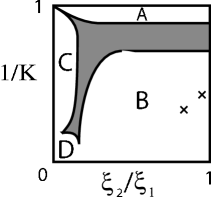
Figure 1: Regions of validity of the approximations presented in Sects. IV A-D in the space of parameters $1/K$ and $\xi_{{}_{2}}/\xi_{{}_{1}}$. In the shaded region, the approximations have a low accuracy; the boundaries are drawn on a qualitative basis. The crosses denote values corresponding to the experiments of Ref. papp2 .

IV.1 Weak Segregation

For the regime of weak segregation i.e. close to the point where the two phases tend to mix ($K\rightarrow 1$), it was found by Barankov in Ref. barankov, that the interface tension varies as:

$$\gamma_{{}_{12}}=4P\xi_{{}_{1}}\frac{\sqrt{K-1}}{3}\left(\frac{1-[\xi_{{}_{2}}/\xi_{{}_{1}}]^{3}}{1-[\xi_{{}_{2}}/\xi_{{}_{1}}]^{2}}\right).$$ (16)

In case of $\xi_{{}_{2}}/\xi_{{}_{1}}=1$, the same leading behavior was recovered in Refs. mazets, , malomed, and ao, and the square-root behavior as a function of $K-1$ arises from simple models as given in Refs. timmermans, and ao, . Approximation (16) is exact at $K=1$ but is already $3.6\%$ off at $K=1.1$ when $\xi_{{}_{2}}=\xi_{{}_{1}}$. Despite this small range of validity, such small values for $K-1$ were realized in the early experiments on phase-segregated ⁸⁷Rb mixtures stenger ; hall ; miesner ; stamper . On the other hand, the use of an interface tension for determining the excess energy in these experiments is inaccurate as the “interface thickness”, that is $\xi_{{}_{1}}/\sqrt{K-1}$, is of the same order as the length of variation of the trapping potential; this invalidates the assumption of constant chemical potentials across the interface.

IV.2 Strong Segregation

In the following we develop an expansion around the point of strong segregation where $1/K\rightarrow 0$. An analogous expansion which originated in a paper by Ginzburg and Landau ginzburg , was used to determine an accurate analytical expression for the interface tension of a normal-superconducting interface boulter .

In the limit $1/K\rightarrow 0$, species $1$ and $2$ do not overlap. Their wave functions are easily found using the GP Eqs. (10) and the boundary conditions (11): $\psi_{{}_{1}}=\Theta(z)\tanh[z/\sqrt{2}\xi_{{}_{1}}]$ and $\psi_{{}_{2}}=\Theta(-z)\tanh[-z/\sqrt{2}\xi_{{}_{2}}]$, where $\Theta$ is the Heaviside function. For a finite but small value of $1/K$, these $\tanh$ profiles shift towards each other so as to overlap over a length proportional to $\sqrt{\xi_{{}_{1}}\xi_{{}_{2}}}/\sqrt[4]{K}$. In this overlap zone, the wave functions are modified due to the interspecies interactions. In Fig. 2B, we depict such wave functions for the case of $\xi_{{}_{2}}/\xi_{{}_{1}}=1$. Note that the length of overlap vanishes very slowly when $1/K\rightarrow 0$ as it is proportional to $1/\sqrt[4]{K}$. We introduce the following (change of) variables ($i=1,2$):

$$\widehat{z}\equiv z/\varsigma_{{}_{0}},\quad\quad\varsigma_{{}_{0}}\equiv\frac{\sqrt{\xi_{{}_{1}}\xi_{{}_{2}}}}{\sqrt[4]{K}}\quad\text{and}\quad\varsigma_{{}_{i}}\equiv\varsigma_{{}_{0}}/\xi_{{}_{i}}.$$ (17)

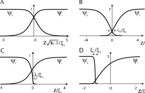
Figure 2: Typical interface profiles for the four cases which are treated in Sects. IVA-D. We indicate the characteristic length scales over which the wave functions vary. A) Weak segregation regime $K\rightarrow 1$ (here with $\xi_{{}_{2}}/\xi_{{}_{1}}=1$). The relevant length scale is $\xi_{{}_{1}}/\sqrt{K-1}$ which is large. B) Strong segregation regime with $1/K\rightarrow 0$ (here with $K=200$ and $\xi_{{}_{2}}/\xi_{{}_{1}}=1$). The condensates overlap over a length scale $\varsigma_{{}_{0}}$ (see Eq. (17)). C) The regime of strong healing length asymmetry $\xi_{{}_{2}}/\xi_{{}_{1}}\rightarrow 0$. When $\xi_{{}_{2}}/\xi_{{}_{1}}$ is small but nonzero, $\psi_{{}_{2}}$ vanishes with a tail of length $\lambda$ (see Eq. (23)). D) When both $\xi_{{}_{2}}/\xi_{{}_{1}}\rightarrow 0$ and $1/K\rightarrow 0$, the condensates will overlap over a distance $\xi_{{}_{2}}$.

Note that $\varsigma_{{}_{0}}$ has the dimension of length (drawn in Fig. 2B) whereas $\varsigma_{{}_{1}}$ and $\varsigma_{{}_{2}}$ are dimensionless. We expand the wave function of phase $i=1,2$ in terms of the parameter $\varsigma_{{}_{i}}$:

$$\psi_{{}_{i}}=\psi_{{}_{i}}^{{}_{0}}+\varsigma_{{}_{i}}(\psi_{{}_{i1}}-\psi_{{}_{i1}}^{{}_{0}})+\varsigma_{{}_{i}}^{3}(\psi_{{}_{i2}}-\psi_{{}_{i2}}^{{}_{0}})+\ldots.$$

We remark that $(\psi_{{}_{i}}-\psi_{{}_{i}}^{{}_{0}})/\varsigma_{{}_{i}}$ is a regular function of $\varsigma_{{}_{i}}^{2}$. The functions $\psi_{{}_{i1}}^{{}_{0}}$ and $\psi_{{}_{i2}}^{{}_{0}}$ are derivable from the asymptotic behavior of $\psi_{{}_{i}}$ for $|\widehat{z}|\rightarrow\infty$ which are shifted $\tanh$ profiles:

$$\psi_{{}_{1}}^{{}_{0}} =\Theta(\widehat{z}+\delta_{{}_{11}}+\varsigma_{{}_{1}}^{2}\delta_{{}_{12}}+\ldots)$$

$$\quad\quad\times\tanh\left[\frac{\varsigma_{{}_{1}}(\widehat{z}+\delta_{{}_{11}}+\varsigma_{{}_{1}}^{2}\delta_{{}_{12}}+\ldots)}{\sqrt{2}}\right]$$

$$\equiv\varsigma_{{}_{1}}\psi_{{}_{11}}^{{}_{0}}+\varsigma_{{}_{1}}^{3}\psi_{{}_{12}}^{{}_{0}}+\ldots$$ (18a)

$$\psi_{{}_{2}}^{{}_{0}} =\Theta(-\widehat{z}+\delta_{{}_{21}}+\varsigma_{{}_{2}}^{2}\delta_{{}_{22}}+\ldots)$$

$$\quad\quad\times\tanh\left[\frac{\varsigma_{{}_{2}}(-\widehat{z}+\delta_{{}_{21}}+\varsigma_{{}_{2}}^{2}\delta_{{}_{22}}+\ldots)}{\sqrt{2}}\right]$$

$$\equiv\varsigma_{{}_{2}}\psi_{{}_{21}}^{{}_{0}}+\varsigma_{{}_{2}}^{3}\psi_{{}_{22}}^{{}_{0}}+\ldots$$ (18b)

From this expansion, it is clear that $\psi_{{}_{i1}}^{{}_{0}}$ and $\psi_{{}_{i2}}^{{}_{0}}$ are first-order and third-order polynomials in $\widehat{z}$ respectively. Note that the “absolute shift” can be set to zero at every order without any loss of generality; thus $\delta_{{}_{11}}=\delta_{{}_{21}}$ and $\varsigma_{{}_{1}}^{2}\delta_{{}_{12}}=\varsigma_{{}_{2}}^{2}\delta_{{}_{22}}$ boulter .

Substitution of the expanded wave functions in the GP Eqs. (10) entails four new differential equations:

$$\ddot{\psi}_{{}_{11}} =\psi_{{}_{11}}\psi_{{}_{21}}^{2},$$ (19a)

$$\ddot{\psi}_{{}_{21}} =\psi_{{}_{21}}\psi_{{}_{11}}^{2},$$ (19b)

$$\ddot{\psi}_{{}_{12}} =-\psi_{{}_{11}}+\psi_{{}_{12}}\psi_{{}_{21}}^{2}+2\psi_{{}_{11}}\psi_{{}_{21}}\psi_{{}_{22}}[\xi_{{}_{2}}/\xi_{{}_{1}}]^{-2},$$ (19c)

$$\ddot{\psi}_{{}_{22}} =-\psi_{{}_{21}}+\psi_{{}_{22}}\psi_{{}_{11}}^{2}+2\psi_{{}_{21}}\psi_{{}_{11}}\psi_{{}_{12}}[\xi_{{}_{2}}/\xi_{{}_{1}}]^{2}.$$ (19d)

Here the dot denotes the derivative with respect to $\widehat{z}$. The solutions of these equations will provide us with the numerical values for the $\delta$’s; indeed, the boundary conditions for $\psi_{{}_{i1}}$ and $\psi_{{}_{i2}}$ are to tangentially approach $\psi_{{}_{i1}}^{{}_{0}}$ and $\psi_{{}_{i2}}^{{}_{0}}$ respectively for $\widehat{z}\rightarrow\pm\infty$, and to vanish for $\widehat{z}\rightarrow\mp\infty$. Now, in the same fashion as the wave functions, one can expand the interface tension:

$$\gamma_{{}_{12}} =\gamma^{{}_{0}}+\varsigma_{{}_{0}}\sum_{i=1,\,2}\left[\gamma_{{}_{i1}}-\gamma^{{}_{0}}_{{}_{i1}}+\varsigma_{{}_{i}}^{2}(\gamma_{{}_{i2}}-\gamma^{{}_{0}}_{{}_{i2}})+\mathcal{O}(\varsigma_{{}_{i}}^{4})\right].$$

The zeroth-order term is obtained using (unshifted) $\tanh$ profiles such that $\gamma^{{}_{0}}=4\sqrt{2}P\left(\xi_{{}_{1}}+\xi_{{}_{2}}\right)/3$ ao ; barankov , while:

$$\sum_{i=1,\,2}\gamma_{{}_{i1}} =4P\int_{{}_{-\infty}}^{{}_{\infty}}\text{d}\widehat{z}\,\left(\dot{\psi}_{{}_{11}}^{2}+\dot{\psi}_{{}_{21}}^{2}\right),$$

$$\sum_{i=1,\,2}\varsigma_{{}_{i}}^{2}\gamma_{{}_{i2}} =\frac{8P}{\sqrt{K}}\int_{{}_{-\infty}}^{{}_{\infty}}\text{d}\widehat{z}\,\left([\xi_{{}_{2}}/\xi_{{}_{1}}]\dot{\psi}_{{}_{11}}\dot{\psi}_{{}_{12}}+\frac{\dot{\psi}_{{}_{21}}\dot{\psi}_{{}_{22}}}{[\xi_{{}_{2}}/\xi_{{}_{1}}]}\right).$$

After long calculations, one can express the interface tension in terms of the spatial shifts $\delta_{{}_{11}}$, $\delta_{{}_{12}}$, $\delta_{{}_{21}}$ and $\delta_{{}_{22}}$, in a way similar to what was done in Ref. boulter, :

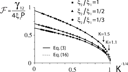
Figure 3: Values of $\mathcal{F}$ or interface tension $\gamma_{{}_{12}}$ in units of $4P\xi_{{}_{1}}$, against values of $K^{-1/4}$ where $K=G_{{}_{12}}/\sqrt{G_{{}_{11}}G_{{}_{22}}}$. The squares, triangles and dots are obtained by numerical integration of the GP equations for $\xi_{{}_{2}}/\xi_{{}_{1}}=1,1/2$ and $1/3$ respectively. The full lines are plots of Eq. (3) and are seen to give an accurate approximation for values of K in the interval $[1.5,\,\infty[$. The grey lines plot Eq. (16) which is accurate for $K\in[1,1.1]$.

$$\gamma_{{}_{12}}=4P\xi_{{}_{1}} \left[\frac{\sqrt{2}}{3}\left(1+\xi_{{}_{2}}/\xi_{{}_{1}}\right)-\frac{(\delta_{{}_{11}}+\delta_{{}_{21}})}{3}\frac{\sqrt{\xi_{{}_{2}}/\xi_{{}_{1}}}}{\sqrt[4]{K}}\right.$$

$$\quad\left.-\frac{\sqrt{\xi_{{}_{2}}/\xi_{{}_{1}}}\left(\delta_{{}_{12}}[\xi_{{}_{2}}/\xi_{{}_{1}}]+\delta_{{}_{22}}[\xi_{{}_{1}}/\xi_{{}_{2}}]\right)}{\sqrt[4]{K}\sqrt{K}}+\ldots\right].$$

It is readily seen in the expansion that $\gamma_{{}_{12}}$ is symmetrical in $\xi_{{}_{1}}$ and $\xi_{{}_{2}}$, as it must be. As a final step, we extracted numerical values for the $\delta$’s from the numerical integration of Eqs. (19). We find that $\delta_{{}_{11}}=\delta_{{}_{21}}=0.771$ boulter , and, assuming $\xi_{{}_{2}}/\xi_{{}_{1}}=1$ in Eqs. (19c) and (19d), we obtain $\delta_{{}_{12}}=\delta_{{}_{22}}=0.055$. Note that this result is different from $\delta_{{}_{2}}$ found in Ref. boulter, because the problem at hand is different starting from the first order in $\varsigma_{{}_{i}}^{2}$. By fitting numerically-obtained values for $\gamma_{{}_{12}}$ with an additional fitting term of fifth order in $1/\sqrt[4]{K}$, and neglecting the dependence of $\delta_{{}_{12}}$ and $\delta_{{}_{22}}$ on $\xi_{{}_{2}}/\xi_{{}_{1}}$, we finally arrive at expression (3).

The accuracy of this expansion is clear from Fig. 3 where we plot Eq. (3) in full lines against the numerically obtained values for $\xi_{{}_{2}}/\xi_{{}_{1}}=1$ (squares), $\xi_{{}_{2}}/\xi_{{}_{1}}=1/2$ (triangles) and $\xi_{{}_{2}}/\xi_{{}_{1}}=1/3$ (dots). Our expansion works very well for $K$ in the interval $[1.5,\,+\infty[$; moreover, it is good for all three values of $\xi_{{}_{2}}/\xi_{{}_{1}}$, which a posteriori justifies the neglect of the dependence of $\delta_{{}_{12}}$, $\delta_{{}_{22}}$ and the fitted higher-order term on $\xi_{{}_{2}}/\xi_{{}_{1}}$. Also in Fig. 3, we draw with grey lines Barankov’s approximation (16), accurate for values of $K$ between $1$ and $1.1$.

IV.3 Strong Healing Length Asymmetry

So far, we have constructed expansions around extreme values for the interspecies interaction parameter $K$. In the following, we will focus on the case when the healing length of species $2$ is much smaller than the one of species $1$ i.e. when $\xi_{{}_{2}}/\xi_{{}_{1}}\ll 1$.

In the limit of $\xi_{{}_{2}}/\xi_{{}_{1}}=0$ (and such that $\xi_{{}_{2}}^{2}\ddot{\psi}_{{}_{2}}\rightarrow 0$), the GP Eqs. (10) can be reduced to

$$\psi_{{}_{2}}^{2}= \,\Theta(-z)\left[1-K\psi_{{}_{1}}^{2}\right],$$ (20a)

$$\xi_{{}_{1}}^{2}\ddot{\psi}_{{}_{1}}= \,\Theta(z)\psi_{{}_{1}}\left[-1+\psi_{{}_{1}}^{2}\right]$$

$$+\Theta(-z)\psi_{{}_{1}}(K-1)\left[1-(1+K)\psi_{{}_{1}}^{2}\right],$$ (20b)

from which it follows that the density of phase $2$ is slaved to the density of phase $1$. The solution to Eq. (20b) is alexandrov :

$$\psi_{{}_{1}} =\Theta(z)\tanh\left(\frac{z+z_{{}_{1}}}{\sqrt{2}\xi_{{}_{1}}}\right)$$ (21)

$$\,\quad+\frac{\Theta(-z)\sqrt{2}}{\sqrt{K+1}}\left[\cosh\left(\frac{z+z_{{}_{2}}}{\xi_{{}_{1}}/\sqrt{K-1}}\right)\right]^{-1}.$$

The constants $z_{{}_{1}}>0$ and $z_{{}_{2}}<0$ are determined by the continuity of $\psi_{{}_{1}}$ at $z=0$ where $\psi_{{}_{1}}^{2}(0)=1/K$. The wave function $\psi_{{}_{2}}$ is nonzero only when $z<0$ and relates to $\psi_{{}_{1}}$ by Eq. (20a). Near $z=0$ it vanishes with the square-root behavior $\psi_{{}_{2}}\propto\sqrt{-z/\xi_{{}_{1}}}$.

The first-order corrections due to a small and nonzero $\xi_{{}_{2}}/\xi_{{}_{1}}$ affect only $\psi_{{}_{2}}$, near the origin $z=0$ where $\ddot{\psi}_{{}_{2}}$ is large due to the square-root behavior of $\psi_{{}_{2}}$. These corrections will induce wave function $\psi_{{}_{2}}$ to acquire a small tail of length $\lambda$ which is depicted Fig. 2C. We search now how GP Eq. (10b) can be modified to appropriately describe such corrections. We assume that $\psi_{{}_{1}}$ varies little on the length scale $\lambda$; this allows to expand $K\psi_{{}_{1}}^{2}$ in Eq. (10b) around $z=0$ as $K\psi_{{}_{1}}^{2}\approx 1+Fz/\xi_{{}_{1}}$ where $F\equiv\sqrt{2/K}(K-1)$. Sufficiently far from the origin, when $\lambda\ll-z\ll\xi_{{}_{1}}$, we want $\psi_{{}_{2}}$ to vary as $\psi_{{}_{2}}\propto\sqrt{-z/\xi_{{}_{1}}}$; therefore, we may not throw away the nonlinear term $\psi_{{}_{2}}^{3}$ in Eq. (10b). By appropriately scaling $\psi_{{}_{2}}$ and $z$, we find that, for $|z|\ll\xi_{{}_{1}}$,

$$\ddot{\overline{\psi}}_{{}_{2}} =\overline{\psi}_{{}_{2}}(\overline{z}+\overline{\psi}_{{}_{2}}^{2}),$$ (22)

where the dot denotes the derivative with respect to $\overline{z}$ which we define as:

$$\overline{z}\equiv z/\lambda\quad\text{with}\quad\lambda\equiv\xi_{{}_{2}}[F[\xi_{{}_{2}}/\xi_{{}_{1}}]]^{-1/3},$$ (23)

and where the new wave function $\overline{\psi}_{{}_{2}}\equiv\psi_{{}_{2}}[F[\xi_{{}_{2}}/\xi_{{}_{1}}]]^{-1/3}$. For $-\overline{z}\gg\lambda$, the term $\ddot{\overline{\psi}}_{{}_{2}}$ in Eq. (22) may be neglected; indeed, doing so results in the solution $\overline{\psi}_{{}_{2}}=\sqrt{-\overline{z}}$. As expected this is in fact $\psi_{{}_{2}}\propto-\sqrt{z/\xi_{{}_{1}}}$.

The differential equation which appears in Eq. (22) was encountered earlier by Lundh et al. lundh and Dalfovo et al. dalfovo when studying the BEC order parameter at the border of a large harmonic trap. The role of the trapping potential is played here by the interactions with condensate $1$.

We briefly sketch how we calculated the interface tension; we refer to Refs. dalfovo, and lundh, for details of the method. To zeroth order in $\xi_{{}_{2}}/\xi_{{}_{1}}$, the interface tension is easily found by integration of $\dot{\psi}_{{}_{1}}^{2}$ (see Eq. (III)) with $\psi_{{}_{1}}$ given in Eq. (21). For small and nonzero $\xi_{{}_{2}}/\xi_{{}_{1}}$, extra energy contributions arise due to the integral over $\dot{\psi}_{{}_{2}}^{2}$ (see Eq. (III)). For $-z\gg\lambda$, $\psi_{{}_{2}}$ must be taken from Eqs. (20a) and (21) whereas for $|z|\ll\xi_{{}_{1}}$, $\psi_{{}_{2}}$ is the (numerical) solution of Eq. (22). Since these two solutions for $\psi_{{}_{2}}$ are equal in the region $\lambda\ll-z\ll\xi_{{}_{1}}$, where $\psi_{{}_{2}}\propto\sqrt{-z/\xi_{{}_{1}}}$ the interface tension is well-defined. All the extra energy contributions due to a nonzero $\xi_{{}_{2}}/\xi_{{}_{1}}$ can be seen to be of order $[\xi_{{}_{2}}/\xi_{{}_{1}}]^{2}$.

Calculations then lead to $\mathcal{F}$ to second order in $\xi_{{}_{2}}/\xi_{{}_{1}}$:

$$\frac{\gamma_{{}_{12}}}{4\xi_{{}_{1}}P}= \frac{2}{3}\frac{\sqrt{K-1}}{K+1}\left[1-\left(\frac{K-1}{2K}\right)^{3/2}\right]+\frac{\sqrt{2}}{3}\left(1+\frac{1}{2}\left(\frac{1}{K}\right)^{3/2}-\frac{3}{2\sqrt{K}}\right)+[\xi_{{}_{2}}/\xi_{{}_{1}}]^{2}\frac{\sqrt{K-1}}{3}\left(\frac{K+3}{K+1}\right)$$

$$+[\xi_{{}_{2}}/\xi_{{}_{1}}]^{2}\frac{(K-1)}{\sqrt{2K}}\left[-\frac{2}{3}\frac{(K+2)}{(K+1)}+0.7+\frac{\ln}{6}\left(\frac{32K(K-1)}{(K+1)^{3}[\xi_{{}_{2}}/\xi_{{}_{1}}]^{2}}\right)-\text{arctanh}\left(\sqrt{\frac{K-1}{2K}}\right)\right]+\ldots$$ (24)

Since there are two length scales ($\lambda$ and $\xi_{{}_{1}}$) over which the density varies, their relation $\lambda\ll\xi_{{}_{1}}$ renders difficult the full numerical integration of the GP Eqs. Accordingly, we could not verify expansion (IV.3) directly.

Conditions for the validity of the above approximation can be derived. First, the linearization of $\psi_{{}_{1}}$ near $z=0$ in Eq. (10b) is justified only when the length over which higher-order corrections to $\psi_{{}_{1}}$ are relevant (that is $[\dot{\psi}_{{}_{1}}/\ddot{\psi}_{{}_{1}}](0)\propto\sqrt{K}\xi_{{}_{1}}$) is large as compared to the length over which $\psi_{{}_{2}}$ varies (being $\lambda$). Second, corrections to $\psi_{{}_{1}}$ caused by a nonzero $\xi_{{}_{2}}/\xi_{{}_{1}}$ can be neglected on $[-\lambda,\infty[$ when, in Eq. (10a), the amplitude $K\psi_{{}_{2}}^{2}$ of the term $K\psi_{{}_{2}}^{2}\psi_{{}_{1}}$ (being $K[F[\xi_{{}_{2}}/\xi_{{}_{1}}]]^{2/3}$) is sufficiently small. These conditions of validity amount to:

$$\xi_{{}_{2}}/\xi_{{}_{1}}\ll\sqrt{K(K-1)}\quad\text{and}\quad\xi_{{}_{2}}/\xi_{{}_{1}}\ll\sqrt{K}.$$

Thus, our expansion fails in the regime of strong segregation when $\sqrt{K}\ll\xi_{{}_{2}}/\xi_{{}_{1}}$ and close to weak segregation when $\sqrt{K-1}\ll\xi_{{}_{2}}/\xi_{{}_{1}}$. Note that to zeroth order in $\xi_{{}_{2}}/\xi_{{}_{1}}$, our expansion (IV.3) agrees with (16) when $K\rightarrow 1$. However, it differs from the expansion (16) by a factor of $2$ in the term of order $[\xi_{{}_{2}}/\xi_{{}_{1}}]^{2}$.

IV.4 Both Strong Segregation and Strong Healing Length Asymmetry

One may now wonder what happens to the interface tension when both $K$ and $[\xi_{{}_{2}}/\xi_{{}_{1}}]^{-1}$ are large. When $K$ goes faster to infinity than $[\xi_{{}_{2}}/\xi_{{}_{1}}]^{-2}$, we will find that expansion (3) is still valid while expansion (IV.3) must be taken in the inverse case. In the following, we focus on the intermediate case when both $[\xi_{{}_{2}}/\xi_{{}_{1}}]^{-2}$ and $K$ diverge such that $\kappa\equiv([\xi_{{}_{2}}/\xi_{{}_{1}}]\sqrt{K})^{-1}$ remains of order one. To zeroth order in both $\xi_{{}_{2}}/\xi_{{}_{1}}$ and $K^{-1}$, the condensate wave functions do not overlap; seen on a lengthscale $\xi_{{}_{1}}$, this results in the wave functions $\psi_{{}_{2}}=\Theta(-z)$ and $\psi_{{}_{1}}=\Theta(z)\tanh[z/\sqrt{2}\xi_{{}_{1}}]$.

For small and nonzero values for $\xi_{{}_{2}}/\xi_{{}_{1}}$ and $1/K$ while $\kappa\equiv([\xi_{{}_{2}}/\xi_{{}_{1}}]\sqrt{K})^{-1}$ is of order one, the condensates overlap. Due to the strong repulsion this happens only within a short region of length $\xi_{{}_{2}}$; over that interval, the value of the wave function $\psi_{{}_{2}}$ varies between zero and one while the value of $\psi_{{}_{1}}$ does not vary much (see Fig. 2D). The latter is only modified close to $z=0$, where, to zeroth order, it vanishes linearly. This brings about the definition of a new wave function $\phi_{{}_{1}}$:

$$\psi_{{}_{1}}=[\xi_{{}_{2}}/\xi_{{}_{1}}]\left[\phi_{{}_{1}}-\frac{z^{\prime}\Theta(z^{\prime})}{\sqrt{2}}\right]+\Theta(z)\tanh\left(\frac{z}{\sqrt{2}\xi_{{}_{1}}}\right).$$

Here we introduced the dimensionless variable $z^{\prime}\equiv z/\xi_{{}_{2}}$ and $\phi_{{}_{1}}$ must have the asymptotic behavior $\phi_{{}_{1}}(z^{\prime}\rightarrow\infty)=z^{\prime}/\sqrt{2}$ and $\phi_{{}_{1}}(z^{\prime}\rightarrow-\infty)=0$. We can now expand the GP Eqs. (10) in terms of the small parameters $[\xi_{{}_{2}}/\xi_{{}_{1}}]^{2}$ and $1/K$ in the overlap interval:

$$\frac{\ddot{\phi}_{{}_{1}}}{\phi_{{}_{1}}}= \left(\frac{\psi_{{}_{2}}}{\kappa}\right)^{2}\quad\text{and}\quad\frac{\ddot{\psi}_{{}_{2}}}{\psi_{{}_{2}}}=-1+\psi_{{}_{2}}^{2}+\left(\frac{\phi_{{}_{1}}}{\kappa}\right)^{2}.$$ (25)

The dots denote the derivative with respect to $z^{\prime}$. One may notice that these equations are the same as the Ginzburg-Landau equations which are valid in a superconductor when a constant magnetic field is applied parallel to its surface. In that case, the Ginzburg-Landau parameter $\kappa$ is the ratio of the penetration length of the magnetic field to the coherence length, $\psi_{{}_{2}}$ plays the role of the order parameter of the superconductor and $\phi_{{}_{1}}$ that of the vector potential .

By a straightforward calculation, one can rewrite the interface tension Eq. (III) as an integral over $\phi_{{}_{1}}$ and $\psi_{{}_{2}}$:

$$\frac{\gamma_{{}_{12}}}{4\xi_{{}_{1}}P}= \frac{\sqrt{2}}{3}+[\xi_{{}_{2}}/\xi_{{}_{1}}]\int\text{d}z^{\prime}\,\left[\left(\dot{\phi}_{{}_{1}}-\frac{1}{\sqrt{2}}\right)^{2}+\dot{\psi}_{{}_{2}}^{2}\right],$$ (26)

where the dots denote the derivative with respect to $z^{\prime}$ and $\phi_{{}_{1}}$ and $\psi_{{}_{2}}$ are obtained by the Euler-Lagrange Eqs. (25).

An analytical expression for the interface tension of a superconductor-normal interface in case of small $\kappa$ was obtained by Boulter and Indekeu in Ref. boulter, . Using their result, one finds:

$$\frac{\gamma_{{}_{12}}}{4P\xi_{{}_{1}}}= \frac{\sqrt{2}}{3}+[\xi_{{}_{2}}/\xi_{{}_{1}}]\left(\frac{\sqrt{2}}{3}-\frac{0.5140}{([\xi_{{}_{2}}/\xi_{{}_{1}}]\sqrt{K})^{1/2}}\right.$$ (27)

$$\left.-\frac{0.06653}{([\xi_{{}_{2}}/\xi_{{}_{1}}]\sqrt{K})^{3/2}}+\frac{0.00107}{([\xi_{{}_{2}}/\xi_{{}_{1}}]\sqrt{K})^{5/2}}+\ldots\right).$$

This approximation is very accurate for values of $\kappa$ in the interval between $0$ and $1$ boulter . To first order in $\kappa$, Eq. (27) agrees with the interface tension found for $K\rightarrow\infty$ as given in Eq. (3).

For large $\kappa$, according to standard results, the integral in Eq. (26) goes as $2(1-\sqrt{2})\kappa/3$ such that saintjames :

$$\frac{\gamma_{{}_{12}}}{4P\xi_{{}_{1}}}= \frac{\sqrt{2}}{3}+\frac{2(1-\sqrt{2})}{3\sqrt{K}}+[\xi_{{}_{2}}/\xi_{{}_{1}}]\mathcal{O}(\kappa^{-1}).$$ (28)

Since large $\kappa$ implies $\xi_{{}_{2}}/\xi_{{}_{1}}\ll\sqrt{K}$, this last result is in full accord with the $K\rightarrow\infty$ limit in expansion Eq. (IV.3). The higher-order corrections to Eq. (28) can also be extracted from Eq. (IV.3).

Note that Eqs. (25) and (27) are valid for all values of $\kappa$ and may be generally used to numerically integrate the interface tension in the limit under consideration.

V Temperature Dependence of the Interface Tension

At low but nonzero temperature, interface waves will be excited as thermal excitations. In the following section, we will consider these and ignore quantum fluctuations. It is common to incorporate the free energy contributions which arise from capillary excitations into a new temperature-dependent interface tension $\gamma_{{}_{12}}(T)$. Generally, when the interface waves have wavenumbers $k$ and frequencies $\omega(k)$, one finds for a three-dimensional system that atkins ; landau4 :

$$\gamma_{{}_{12}}(T)=\gamma_{{}_{12}}(0)+\frac{k_{{}_{B}}T}{2\pi}\int_{{}_{0}}^{{}_{\infty}}\ln\left(1-e^{-\hslash\omega(k)/k_{{}_{B}}T}\right)k\text{d}k,$$

where $\gamma_{{}_{12}}(0)$ is the interface tension at zero temperature and the last term embodies a negative correction due to a nonzero temperature. For a flat interface between two BECs, one may obtain the capillary-wave spectrum from the time-dependent GP Eqs. For sufficiently large wavelengths $k^{-1}\gg\gamma_{{}_{12}}/P$, one then finds for the modes with in-phase motion of both species mazets ; barankov :

$$\omega(k)=k^{3/2}\sqrt{\frac{\gamma_{{}_{12}}}{m_{{}_{1}}n_{{}_{1}}+m_{{}_{2}}n_{{}_{2}}}},$$ (29)

where $n_{i}$ is the bulk density of phase $i=1,\,2$. When the temperature $T$ satisfies the condition $k_{{}_{B}}T\ll\hslash^{2}/(2m_{{}_{i}}(\gamma_{{}_{12}}/P)^{2})$, only modes with wavenumbers satisfying Eq. (29) are thermally excited. The temperature-dependent interface tension then becomes :

$$\gamma_{{}_{12}}(T)=\gamma_{{}_{12}}(0)-\frac{c\left(k_{{}_{B}}T\right)^{7/3}}{4\pi\hslash^{4/3}}\left(\frac{m_{{}_{1}}n_{{}_{1}}+m_{{}_{2}}n_{{}_{2}}}{\gamma_{{}_{12}}(0)}\right)^{2/3},$$

where $c\equiv\Gamma(7/2)\zeta(7/2)$ and $\zeta$ and $\Gamma$ are the zeta and gamma function, respectively.

Taking $n_{{}_{1}}\approx n_{{}_{2}}$, $\gamma_{{}_{12}}(0)\propto\xi_{{}_{1}}P$ and $\mu_{{}_{1}}\approx\mu_{{}_{2}}$, one calculates that the relative temperature corrections $[\gamma_{{}_{12}}(T)-\gamma_{{}_{12}}(0)]/\gamma_{{}_{12}}(0)$ are of order $\sqrt{n_{{}_{1}}a_{{}_{11}}^{3}}(k_{{}_{B}}T/\mu_{{}_{1}})^{7/3}$. It is known that $\sqrt{n_{{}_{1}}a_{{}_{11}}^{3}}\ll 1$ is the condition for the GP theory to be applicable; moreover for the current BEC experiments $k_{{}_{B}}T$ is of the same order or less than $\mu_{{}_{1}}$ pita .

On the other hand, for a system in the weakly segregated regime, the interface tension varies as $\gamma_{{}_{12}}(0)\propto\xi_{{}_{1}}P\sqrt{K-1}$ and accordingly vanishes as $K\rightarrow 1$. The relative temperature corrections are then of order $(K-1)^{-5/6}\sqrt{n_{{}_{1}}a_{{}_{11}}^{3}}(k_{{}_{B}}T/\mu_{{}_{1}})^{7/3}$ which may become large as $K\rightarrow 1$.

In conclusion, thermal fluctuations of a flat BEC interface do not affect the interface tension at low temperature, except possibly near weak segregation. Note that the calculated temperature dependence of the interface tension does not hold in trapped systems, as the interface modes there are quantized svidzinsky ; lazarides .

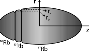
Figure 4: Cross section of a trapped cloud of BEC mixtures as it was observed in Ref. papp2, . Due to phase segregation, ⁸⁵Rb forms a layer between clouds of ⁸⁷Rb. In Eq. (30), we calculate the total excess energy due to the presence of the two interfaces.

VI Discussion

We discuss now the relevance of our results with respect to the recent experiments of Papp et al. papp2 . Two main values for the scattering lengths of phase-segregated states were reported: one configuration was characterized by $K=3.01$ and $\xi_{{}_{2}}/\xi_{{}_{1}}=0.84$ such that $\mathcal{F}=\gamma_{{}_{12}}/(4P\xi_{{}_{1}})=0.434$, while for the other configuration, $K=2.36$ and $\xi_{{}_{2}}/\xi_{{}_{1}}=0.952$ such that $\mathcal{F}=0.415$. Here species $1$ and $2$ are ⁸⁵Rb and ⁸⁷Rb respectively. Note that these values for $\mathcal{F}$ are obtained both numerically and with Eq. (3). The values for $\mathcal{F}$ together with Eq. (1) allow a numerical calculation of the interface excess of any trapped configuration.

As an example, we consider now the topology as depicted in Fig. 4 in which a layer of ⁸⁵Rb BEC is present between clouds of ⁸⁷Rb. This configuration was experimentally obtained in Ref. papp2, by strong radial confinement so as to quench gravitational effects. Particles of phase $i=1,2$ are confined by an anisotropic trapping potential $U_{{}_{i}}(r,z)=m_{{}_{i}}(\omega^{2}_{{}_{ri}}r^{2}+\omega^{2}_{{}_{zi}}z^{2})/2$ with $r^{2}=x^{2}+y^{2}$. Using Eq. (1), one finds the total excess energy due to the presence of the two interfaces:

$$\Omega_{\mathcal{A}}^{{}_{HO}}=\mathcal{F}(\xi_{{}_{2}}/\xi_{{}_{1}},K)\frac{m_{{}_{1}}^{2}\omega_{{}_{r1}}^{3}(r_{{}_{a}}^{5}+r_{{}_{b}}^{5})}{20\hslash a_{{}_{11}}}.$$ (30)

Here $r_{{}_{a}}$ and $r_{{}_{b}}$ are the maximal radial coordinates along the two interfaces (see Fig. 4) and $\mathcal{F}=0.415$. Comparing this excess energy $\Omega_{\mathcal{A}}^{{}_{HO}}$ with the total energy $E$ of a gas of $1.4\times 10^{5}$ ⁸⁷Rb particles, we obtain that $\Omega_{\mathcal{A}}^{{}_{HO}}/E\approx 0.03$. This implies that, even for the largest clouds observed in Ref. papp2, , the interface excess energy is substantial and must be considered accurately when determining the shape of the ground state configuration.

Note that in recent experiments on ultracold imbalanced fermion gases, a breaking of the local density approximation was encountered in the sense that the introduction of the interface and its tension was essential in explaining the experiments partridge ; vanschaeybroeck .

The formalism presented in this work assumes a local approximation for the interface tension. For this approach to be valid, the interface thickness must be smaller than the length over which the trapping potential varies. Generally, the former length is simply $\xi_{{}_{1}}+\xi_{{}_{2}}$; however, close to the mixed state (i.e. when $K\rightarrow 1$) it is $(\xi_{{}_{1}}+\xi_{{}_{2}})/\sqrt{K-1}$ which is larger. On the other hand, the characteristic variation length of the trapping potential of species $i$ is $a_{{}_{ho}}=\sqrt{\hslash/m_{{}_{i}}\overline{\omega}_{{}_{i}}}$ with $\overline{\omega}\equiv(\omega_{{}_{r,i}}^{2}\omega_{{}_{z,i}})^{1/3}$. If we consider the configuration of $1.4\times 10^{5}$ particles with $K=2.36$ and $\xi_{{}_{2}}/\xi_{{}_{1}}=0.952$, we find that $(\xi_{{}_{1}}+\xi_{{}_{2}})/a_{{}_{ho}}\approx 0.1$ is indeed small at the trap center papp2 . Although the coherence lengths diverge at the trap boundary, this divergence is so weak that $\xi_{{}_{1}}+\xi_{{}_{2}}$ exceeds $a_{{}_{ho}}$ only in a layer of thickness of $0.5\%$ of the trapping radius. This justifies the use of the local approximation for the interface in the experiments of Ref. papp2, .

VII Conclusion

We propose a method to calculate the total energy of a trapped phase-segregated BEC mixture. In order to find the bulk energies, one can use a local density approximation or Thomas-Fermi approach. However, with respect to the recent experiments on phase-segregated BEC components papp2 , the bulk contribution must be supplemented by interface excesses which may have pronounced effects on the ground state topology. The interface excess energy arises from the presence of the two-phase boundaries, the position of which are determined by the Laplace equation. Using a local approximation for the interface, we write the total excess energy as a simple integral of the trapping potential along the interface (see Eq. (1)). By use of analytical expansions, we find the interface tension in almost all parameter regimes (see Fig. 1), including the regimes encountered in Ref. papp2, . We also study the influence of thermal fluctuations on the interface tension at low temperature and find that their effect is negligible, except possibly close to the mixed state.

VIII Acknowledgements

The author acknowledges partial support by Projects Nos. FWO G.0115.06 and GOA/2004/02 and thanks very much Joseph Indekeu for useful discussions, suggestions and a thorough reading of the manuscript. Achilleas Lazarides is thanked for corrections to the manuscript. The author is supported by the Research Fund K.U.Leuven.

References

- (1) C.J. Myatt, E.A. Burt, R.W. Ghrist, E.A. Cornell and C.E. Wieman, Phys. Rev. Lett. 78, 586 (1997).
- (2) M.R. Matthews, B.P. Anderson, P.C. Haljan, D.S. Hall, C.E. Wieman and E.A. Cornell, Phys. Rev. Lett. 83, 2498 (1999).
- (3) G. Modugno, M. Modugno, F. Riboli, G. Roati and M. Inguscio, Phys. Rev. Lett. 89, 190404 (2002).
- (4) H.-J. Miesner, D.M. Stamper-Kurn, J. Stenger, S. Inouye, A.P. Chikkatur and W. Ketterle, Phys. Rev. Lett. 82, 2228 (1999).
- (5) D.M. Stamper-Kurn, H.-J. Miesner, A.P. Chikkatur, S. Inouye, J. Stenger and W. Ketterle, Phys. Rev. Lett. 83, 661 (1999).
- (6) J. Stenger, S. Inouye, D.M. Stamper-Kurn, H.-J. Miesner, A.P. Chikkatur and W. Ketterle, Nature (London) 396, 345 (1998).
- (7) D.S. Hall, M.R. Matthews, J.R. Ensher, C.E. Wieman and E.A. Cornell, Phys. Rev. Lett. 81, 1539 (1998).
- (8) G. Thalhammer, G. Barontini, L. De Sarlo, J. Catani, F. Minardi and M. Inguscio, arXiv:0803.2763.
- (9) S.B. Papp and C.E. Wieman, Phys. Rev. Lett. 97, 180404 (2006).
- (10) S.B. Papp, J.M. Pino and C.E. Wieman, arXiv:0802.2591.
- (11) T.-L. Ho and V.B. Shenoy, Phys. Rev. Lett. 77, 3276 (1996).
- (12) R. Graham and D. Walls, Phys. Rev. A 57, 484 (1998).
- (13) B.D. Esry and C.H. Greene, Phys. Rev. A 57, 1265 (1998).
- (14) B.D. Esry, C.H. Greene, J.P. Burke and J.L. Bohn, Phys. Rev. Lett 78, 3594 (1997).
- (15) P. Öhberg and S. Stenholm, Phys. Rev. A 57, 1272 (1998).
- (16) E.P. Bashkin and A.V. Vagov, Phys. Rev. B, 56, 6207 (1997).
- (17) J.P. Burke, J.L. Bohn, B.D. Esry and C.H. Greene, Phys. Rev. Lett. 80, 2097 (1998).
- (18) F. Riboli and M. Modugno, Phys. Rev. A 65, 063614 (2002).
- (19) D.M. Jezek and P. Capuzzi, Phys. Rev. A 66, 015602 (2002).
- (20) A.S. Alexandrov and V.V. Kabanov, J. Phys.: Condens. Matter 14, L327 (2002).
- (21) E. Timmermans, Phys. Rev. Lett. 81, 5718 (1998); S.G. Bhongale and E. Timmermans, arXiv:0711.4007.
- (22) P. Ao and S.T. Chui, Phys. Rev. A 58, 4836 (1998).
- (23) I.E. Mazets, Phys. Rev. A 65, 033618 (2002).
- (24) R.A. Barankov, Phys. Rev. A 66, 013612 (2002).
- (25) P. Ao and S.T. Chui, J. Phys. B: At. Mol. Opt. Phys. 33 535 (2000).
- (26) S.T. Chui, V.N. Ryzhov and E.E. Tareyeva, JETP 91, 1183 (2000).
- (27) A.A. Svidzinsky and S.T. Chui, Phys. Rev. A 67, 053608 (2003); ibid. 68, 013612 (2003).
- (28) H. Pu and N.P. Bigelow, Phys. Rev. Lett. 80, 1134 (1998).
- (29) Th. Busch, J.I. Cirac, V.M. Pérez-Garcia and P. Zoller, Phys. Rev. A 56, 297 8(1997).
- (30) C.K. Law, H. Pu, N.P. Bigelow and J.H. Eberly, Phys. Rev. Lett. 79, 3105 (1997).
- (31) F. Dalfovo, L. Pitaevskii and S. Stringari, Phys. Rev. A 54, 4213 (1996).
- (32) E. Lundh, C. J. Pethick and H. Smith, Phys. Rev. A 55, 2126 (1997).
- (33) U. Al Khawaja, C.J. Pethick and H. Smith, Phys. Rev. A 60, 1507 (1999).
- (34) A.L. Fetter and D.L. Feder, Phys. Rev. A 58, 3185 (1998).
- (35) Y. Colombe, B. Mercier, H. Perrin, V. Lorent, Phys. Rev. A 72 (2005) 061601(R).
- (36) D. Rychtarik, B. Engeser, H.-C. Nägerl and R. Grimm, Phys. Rev. Lett. 92, 173003 (2004).
- (37) A. Landragin, J.-Y. Courtois, G. Labeyrie, N. Vansteenkiste, C.I. Westbrook and A. Aspect, Phys. Rev. Lett. 77, 1464 (1996).
- (38) J.O. Indekeu and B. Van Schaeybroeck, Phys. Rev. Lett. 93, 210402 (2004).
- (39) A.L. Fetter and J.D. Walecka, Quantum theory of many-particle systems (McGraw Hill, Boston, 1971).
- (40) C.J. Pethick and H. Smith, Bose-Einstein condensation in dilute gases (Cambridge Press, Cambridge, 2002).
- (41) L.P. Pitaevskii and S. Stringari, Bose-Einstein Condensation, Clarendon Press.
- (42) B.A. Malomed, A.A. Nepomnyashchy and M. Tribelsky, Phys. Rev. A 42, 7244 (1990).
- (43) V.L. Ginzburg and L.D. Landau, Zh. Eksp. Teor. Fiz. 20, 1064 (1950).
- (44) C.J. Boulter and J.O. Indekeu, Phys. Rev. B 54, 12407 (1996).
- (45) J.O. Indekeu and J.M.J. van Leeuwen, Physica C 251, 290 (1995).
- (46) D. Saint-James, G. Sarma and E.J. Thomas, Type-II Superconductivity (Pergamon, Oxford, 1969).
- (47) K.R. Atkins, Can. J. Phys. 31, 1165 (1953).
- (48) E.M. Lifshitz and L.P. Pitaevskii. Statistical Mechanics, Part 2 (Pergamon Press, Oxford, 1980).
- (49) G.B. Partridge, W. Li, Y.A. Liao, R.G. Hulet, M. Haque and H.T.C. Stoof, Phys. Rev. Lett. 97, 190407 (2006).
- (50) B. Van Schaeybroeck and A. Lazarides, Phys. Rev. Lett. 98, 170402 (2007).
- (51) A. Lazarides and B. Van Schaeybroeck, Phys. Rev. A 77, 041602(R) (2008).
- (52) W.F. Saam, Phys. Rev. B 12, 16 (1974).