arXiv: cond-mat.soft/0805.2471v2

Characterization of geometric structures
of biaxial nematic phases

Shogo Tanimura      and      Tomonori Koda

¹Department of Applied Mathematics and Physics, Graduate School of Informatics,
Kyoto University, Kyoto 606-8501, Japan

²Graduate School of Science and Engineering,
Yamagata University, Yonezawa 992-8510, Japan

submitted on 16 May 2008, revised on 22 May 2008

Abstract

The ordering matrix, which was originally introduced by de Gennes, is a well-known mathematical device for describing orientational order of biaxial nematic liquid crystal. In this paper we propose a new interpretation of the ordering matrix. We slightly modify the definition of the ordering matrix and call it the geometric order parameter. The geometric order parameter is a linear transformation which transforms a tensorial quantity of an individual molecule to a tensorial quantity observed at a macroscopic scale. The degree of order is defined as the singular value of the geometric order parameter. We introduce the anisotropy diagram, which is useful for classification and comparison of various tensorial quantities. As indices for evaluating anisotropies of tensorial quantities, we define the degree of anisotropy and the degree of biaxiality. We prove that a simple diagrammatic relation holds between a microscopic tensor and a macroscopic tensor. We provide a prescription to formulate the Landau-de Gennes free energy of a system whose constituent molecules have an arbitrary shape. We apply our prescription to a system which consists of $D_{2h}$-symmetric molecules.

PACS codes: 61.30.Cz, 61.30.Gd, 83.80.Xz

Keywords: biaxial nematic phase, ordering matrix, geometric order parameter, anisotropy diagram, degree of anisotropy, degree of biaxiality, micro-macro relation, Landau-de Gennes free energy

1 Introduction

A system which consists of asymmetric molecules can exhibit various noticeable phenomena. In particular, biaxial nematic liquid crystals are interesting subjects of current research. Biaxiality means that physical properties of an individual molecule or an ensemble of molecules are not invariant under any rotations. On the other hand, uniaxiality means that properties of a molecule or an ensemble of molecules are invariant under rotations about a fixed axis. Anisotropy is a general concept which implies either uniaxiality or biaxiality. Although most of molecules are not uniaxially symmetric in a rigorous sense, it is possible that some properties of molecules are effectively uniaxial. In a simple nematic liquid crystal uniaxial molecules are aligned to exhibit a uniaxial order at a macroscopic scale. However, in a more complex system under some circumstance, it may happen that uniaxial molecules exhibit a biaxial order, or it may also happen that biaxial molecules exhibit a biaxial order.

Biaxial nematic phases have been intensively studied in liquid crystal physics. Williams [1] noticed biaxial anisotropy in optical properties of nematic liquid crystals in a magnetic field. Taylor, Fergason, and Arora [2] found a biaxial smectic C phase. Freiser [3] began a theoretical study of phase structures of asymmetric molecules and predicted the existence of a biaxial nematic phase. Alben [4] calculated the Landau free energy of a system of biaxial molecules and predicted the existence of a biaxial phase. Straley [6] introduced four order parameters, $(S,T,U,V)$ in his notation, to describe nematic order structures of an ensemble of molecules which have the point group $D_{2h}$ as their symmetry. de Gennes and Prost [7] introduced a set of generalized order parameters, which is called the ordering matrix, to describe nematic order structures of molecules which have an arbitrary shape. Yu and Saupe [8] observed a biaxial phase in an experiment and obtained a phase diagram in the concentration-temperature coordinate. There the biaxial phase appeared between two distinct uniaxial phases. Boonbrahm and Saupe [9] studied effects of temperature and magnetic field on a thin film of biaxial nematic liquid. Allender, Lee, and Hafiz [10, 11] constructed the Landau-de Gennes free energy of $D_{2h}$-symmetric molecules up to the sixth order in the Straley variables $(S,T,U,V)$. Bunning, Crellin, and Faber [13] studied experimentally an effect of molecular biaxiality on bulk properties, particularly on the magnetic anisotropy. Gramsbergen, Longa, and de Jeu [14] wrote a review on the Landau theory of the nematic-isotropic phase transition. However, the effects of biaxiality of molecules were not sufficiently considered in their review. Remler and Haymet [15] gave a complete formulation for describing interactions between asymmetric molecules and applied their formulation to the analysis of the Landau free energy. Mulder [16] formulated a model of sphero-platelet molecules which interact by exclusive volume effect. Since his model has the $D_{2h}$ symmetry, the order is described by the four order parameters of Straley. Solving the problem by the mean field approximation, he showed that a transition between the isotropic phase and the biaxial phase can occur.

The discoveries of a thermotropic biaxial phase in a system of bent molecules (banana-shaped or boomerang-shaped molecules) by Madsen, Dingemans, Nakata, and Samulski [20] and by Acharya, Primak, and Kumar [21] renewed the interest in biaxial nematics [22]. In their experiments it was observed that biaxial molecules exhibited biaxial orders without application of external fields nor boundary effects. Their discoveries have been stimulating intensive researches in this field [23, 24, 25, 26, 28, 29]. Merkel et al. [23] measured biaxiality parameters by infrared absorbance measurements and compared the observed data with a result of the Landau-de Gennes model. Bates and Luckhurst [24] studied the phase diagram of a liquid which consists of V-shaped molecules by the Monte Carlo simulation. They showed existence of biaxial phases in the diagrams whose coordinates are temperature and various anisotropy parameters like the bending angle of the molecule.

However, for a theoretical analysis of biaxial nematic phases, it seems that there is still a confusion in descriptions of anisotropies. In other words, it is necessary to invent a more useful and comprehensive method for describing anisotropies of molecules and nematic phases. Let us discuss issues which exist in the present method for describing anisotropies of general nematics. For a liquid crystal which consists of uniaxial molecules, a well-known device to characterize orientational order of nematic phase is the tensorial order parameter

$$\mbox{\boldmath$A$}=\Big{\langle}\mbox{\boldmath$n$}\otimes\mbox{\boldmath$n$}-\frac{1}{3}I\Big{\rangle}.$$ (1)

Here $n$ is a unit vector which is fixed along the axis of each molecule and viewed from a laboratory observer. Since the molecules execute thermal motion, the direction of the vector $n$ fluctuates. The brackets $\langle\cdots\rangle$ mean a statistical average. The components of the tensor $A$ are written as

$$A_{ij}=\Big{\langle}n_{i}\,n_{j}-\frac{1}{3}\,\delta_{ij}\Big{\rangle},\qquad i,j=1,2,3.$$ (2)

The eigenvectors and eigenvalues of $A$ indicate alignment of the molecules. The matrix $A$ can be diagonalized and parameterized as

$$\mbox{\boldmath$A$}=\frac{1}{3}\begin{pmatrix}-\sigma+\tau&0&0\\ 0&-\sigma-\tau&0\\ 0&0&2\sigma\end{pmatrix}.$$ (3)

When $\sigma=\tau=0$, the system is in an isotropic phase. When $\sigma\neq 0$ and $\tau=0$, the system is in a uniaxial nematic phase. The value of $\sigma$ is in the range $-\frac{1}{2}\leq\sigma\leq 1$. When $\tau\neq 0$, the system is in a biaxial nematic phase.

If the molecule itself is biaxial, we may introduce another order parameter,

$$\mbox{\boldmath$B$}=\Big{\langle}\mbox{\boldmath$l$}\otimes\mbox{\boldmath$l$}-\mbox{\boldmath$m$}\otimes\mbox{\boldmath$m$}\Big{\rangle}.$$ (4)

Here $\mbox{\boldmath$l$},\mbox{\boldmath$m$},\mbox{\boldmath$n$}$ are mutually orthogonal unit vectors fixed on each molecule. The quantity $B$ characterizes the biaxial anisotropy of the nematic phase. In general, we may associate principal values $\lambda_{1},\lambda_{2},\lambda_{3}$ with the principal axes $\mbox{\boldmath$l$},\mbox{\boldmath$m$},\mbox{\boldmath$n$}$ and define the order parameter

$$\mbox{\boldmath$C$}=\Big{\langle}\lambda_{1}\mbox{\boldmath$l$}\otimes\mbox{\boldmath$l$}+\lambda_{2}\mbox{\boldmath$m$}\otimes\mbox{\boldmath$m$}+\lambda_{3}\mbox{\boldmath$n$}\otimes\mbox{\boldmath$n$}-\frac{1}{3}(\lambda_{1}+\lambda_{2}+\lambda_{3})I\Big{\rangle}.$$ (5)

These order parameters, $A$, $B$, and $C$, are useful for characterizing orientational order structures of nematic phases. But there are several difficulties in their application to molecules which have an arbitrary shape. First, there is no a priori reason to choose the molecular axes $\mbox{\boldmath$l$},\mbox{\boldmath$m$},\mbox{\boldmath$n$}$ for an asymmetric molecule. If the molecule is rectangular, choice of the axes is rather obvious. However, for a molecule which has no symmetry, choice of the axes is not unique. There are various candidates for the molecular axes; we may take the principal axes of the inertia tensor, the dielectric susceptibility tensor, the electric quadrupole tensor, or the magnetic susceptibility tensor of the molecule. In general, the axes defined by them do not coincide. Thus, there is no unique definition of the molecular axes. Second, distinction between the uniaxiality and the biaxiality becomes ambiguous since the eigenvalues of $A$ and $B$ depend on the choice of the molecular axes. Furthermore, there is no reason to choose a unique set of the principal values $\lambda_{1},\lambda_{2},\lambda_{3}$ in the definition of the tensor $C$. Third, the relation between the anisotropy of a molecule and the anisotropy of a macroscopic phase is vague in this kind of analysis. It can happen that uniaxial molecules exhibit a biaxial phase. It is also possible that biaxial molecules exhibit a uniaxial phase. Thus a systematic method to compare the molecular anisotropy and the macroscopic anisotropy is desirable.

de Gennes [7] introduced the ordering matrix

$$S_{abij}=\frac{3}{2}\left\langle R_{ai}\,R_{bj}-\frac{1}{3}\delta_{ab}\,\delta_{ij}\right\rangle,\qquad a,b,i,j=1,2,3$$ (6)

for characterizing alignment of molecules in a nematic phase. Here $R_{ai}=\mbox{\boldmath$L$}_{a}\cdot\mbox{\boldmath$M$}_{i}$ is an inner product of the laboratory orthogonal frame $(\mbox{\boldmath$L$}_{1},\mbox{\boldmath$L$}_{2},\mbox{\boldmath$L$}_{3})$ with the molecular orthogonal frame $(\mbox{\boldmath$M$}_{1},\mbox{\boldmath$M$}_{2},\mbox{\boldmath$M$}_{3})$. The symmetrized tensor

$$G_{abij}=\left\langle\frac{1}{2}(R_{ai}\,R_{bj}+R_{bi}\,R_{aj})-\frac{1}{3}\delta_{ab}\,\delta_{ij}\right\rangle$$ (7)

is more useful and meaningful as will be shown in this paper. Although the ordering matrix is applicable to molecules of an arbitrary shape, it is still difficult to read out geometrical and physical implications from the ordering matrix.

In this paper we introduce a new approach for characterization and analysis of anisotropies of a molecule and a bulk phase. However, here we describe the outline of this paper. In our discussion, the adjective microscopic means intrinsic properties or quantities which an individual molecule possesses. On the other hand, macroscopic means average properties or quantities observed in an ensemble of a large number of molecules. If each molecule has a tensorial quantity $t_{ij}$ and if the molecule changes its direction, the tensor is transformed to $\tilde{t}_{ab}=\sum_{i,j}R_{ai}\,R_{bj}\,t_{ij}$ by a rotation matrix $R_{ai}$. We assume that $t_{ij}$ is a traceless symmetric tensor. The quantity observable at a macroscopic scale is a statistical average $\langle\tilde{t}_{ab}\rangle=\sum_{i,j}\langle R_{ai}\,R_{bj}\rangle\,t_{ij}=\sum_{i,j}G_{abij}\,t_{ij}$. This is an equation defining the geometric order parameter $G_{abij}$. Thus, the geometric order parameter can be regarded as a bridge which relates the microscopic quantity $t_{ij}$ to the macroscopic quantity $\langle\tilde{t}_{ab}\rangle$. Since the geometric order parameter $G=(G_{abij})$ is a linear transformation $\mbox{\boldmath$t$}\mapsto G\mbox{\boldmath$t$}$, its property is completely analyzed by the method of singular value decomposition. In Sect. 2 we will introduce the geometric order parameter and discuss its properties.

After understanding the geometric order parameter, the remaining task is to characterize anisotropies implied by the individual tensors, $t_{ij}$ and $\langle\tilde{t}_{ab}\rangle$. To visualize the anisotropic property of a tensor we introduce an anisotropy diagram, in which each tensor is represented as a point in a plane. Then we define the degree of anisotropy $\alpha(\mbox{\boldmath$t$})$ and the degree of biaxiality $\beta(\mbox{\boldmath$t$})$ of the tensor $\mbox{\boldmath$t$}=(t_{ij})$. Sect. 3 is an introductory discussion for providing the indices of anisotropy and Sect. 4 is an explanation of the anisotropy diagram.

Furthermore, the geometric order parameter enables us to compare anisotropies of the microscopic tensor $t$ and the macroscopic tensor $\langle\tilde{\mbox{\boldmath$t$}}\rangle=G\mbox{\boldmath$t$}$. We found that in the anisotropic diagram there is a simple geometric relation between the microscopic tensor and the corresponding macroscopic tensor. In Sect. 5 we will prove some theorems to ensure the micro-macro relation. This section is a highlight of this paper.

In Sect. 6 we will show simple applications of our method. In Sect. 7 we restrict our consideration to molecules which have the $D_{2h}$ symmetry. Then, we will reproduce the four order parameters of Straley. In Sect. 8 we will give a general prescription to formulate the Landau-de Gennes free energy model. There we refer to the theorem which tells a complete set of ingredients of the Landau-de Gennes free energy. In the appendix we prove the theorem. A real molecule may have various tensorial quantities which are not simultaneously diagonalizable. Our prescription is applicable even to such a general system. Finally, we apply our prescription and obtain a complete Landau-de Gennes free energy for the $D_{2h}$-symmetric molecules. Sect. 9 is devoted to concluding remarks.

We would like to emphasize that our method for characterizing anisotropies is applicable to a general system in which molecules may have arbitrary shapes and arbitrary tensorial quantities. Our method is systematic and unambiguous. The anisotropy diagram will help both qualitative and quantitative understandings of anisotropies. Our prescription for formulating the Landau-de Gennes free energy enables us to construct a complete invariant polynomial which contains neither too many nor too few terms.

2 Geometric order parameter

In this section we introduce the geometric order parameter. Although it is just a modified version of de Gennes’ ordering matrix, it will give a clear and new interpretation of the ordering matrix.

Assume that a molecule has an intrinsic vectorial quantity $\mbox{\boldmath$v$}=(v_{1},v_{2},v_{3})$, which can be, for example, an electric dipole moment. When the molecule rotates, the vector $v$ is transformed to

$$\tilde{\mbox{\boldmath$v$}}=R\mbox{\boldmath$v$},\qquad\mbox{or}\qquad\tilde{v}_{a}=\sum_{i=1}^{3}R_{ai}\,v_{i}$$ (8)

by a three-dimensional orthogonal matrix $R\in SO(3)$. The matrix elements $R_{ai}$ satisfy $\sum_{a}R_{ai}R_{aj}=\delta_{ij}$ and $\sum_{i}R_{ai}R_{bi}=\delta_{ab}$. Each molecule can be transformed by a different rotation matrix. Since liquid crystal is an ensemble of molecules, the quantity observed in the laboratory is the average

$$\langle\tilde{\mbox{\boldmath$v$}}\rangle=\langle R\rangle\mbox{\boldmath$v$},\qquad\mbox{or}\qquad\langle\tilde{v}_{a}\rangle=\sum_{i=1}^{3}\langle R_{ai}\rangle v_{i}.$$ (9)

Once we know the matrix elements $\langle R_{ai}\rangle$, we can calculate the average $\langle\tilde{\mbox{\boldmath$w$}}\rangle=\langle R\rangle\mbox{\boldmath$w$}$ for any vectorial quantity $w$ of the molecule. Most of liquid crystals have no polarity and hence $\langle R_{ai}\rangle$ are usually zero.

Next, assume that the molecule has an intrinsic tensorial quantity $\mbox{\boldmath$t$}=(t_{ij})$, which may be a dielectric susceptibility or an electric quadrupole moment. When the molecule rotates, the tensor $t$ is transformed to

$$\tilde{\mbox{\boldmath$t$}}=(R\otimes R)\mbox{\boldmath$t$},\qquad\mbox{or}\qquad\tilde{t}_{ab}=\sum_{i,j=1}^{3}R_{ai}\,R_{bj}\,t_{ij}.$$ (10)

Any tensor $t$ can be decomposed into the scalar component, the antisymmetric component, and the traceless symmetric component as

$$t_{ij}=\bigg{[}\frac{1}{3}\delta_{ij}\sum_{k=1}^{3}t_{kk}\bigg{]}+\bigg{[}\frac{1}{2}(t_{ij}-t_{ji})\bigg{]}+\bigg{[}\frac{1}{2}(t_{ij}+t_{ji})-\frac{1}{3}\delta_{ij}\sum_{k=1}^{3}t_{kk}\bigg{]}.$$ (11)

If the tensor $t$ is traceless and symmetric, the transformed tensor $\tilde{\mbox{\boldmath$t$}}$ is also traceless and symmetric. Hence we can write the components of $\tilde{\mbox{\boldmath$t$}}$ as

$$\tilde{t}_{ab}=\frac{1}{2}(\tilde{t}_{ab}+\tilde{t}_{ba})-\frac{1}{3}\delta_{ab}\sum_{c=1}^{3}\tilde{t}_{cc}=\sum_{i,j=1}^{3}\bigg{[}\frac{1}{2}(R_{ai}\,R_{bj}+R_{bi}\,R_{aj})-\frac{1}{3}\delta_{ab}\,\delta_{ij}\bigg{]}t_{ij}.$$ (12)

Thus, the transformation law of traceless symmetric tensors is described as

$$\tilde{t}_{ab}=\sum_{i,j=1}^{3}Q_{abij}\,t_{ij}$$ (13)

with the symmetrized traceless matrix

$$Q_{abij}=\frac{1}{2}(R_{ai}\,R_{bj}+R_{bi}\,R_{aj})-\frac{1}{3}\delta_{ab}\,\delta_{ij}.$$ (14)

Then the average, which is an observable at a macroscopic scale, is given by

$$\langle\tilde{\mbox{\boldmath$t$}}\rangle=\langle Q\rangle\mbox{\boldmath$t$}=G\mbox{\boldmath$t$},\qquad\mbox{or}\qquad\langle\tilde{t}_{ab}\rangle=\sum_{i,j=1}^{3}\langle Q_{abij}\rangle t_{ij}=\sum_{i,j=1}^{3}G_{abij}\,t_{ij}.$$ (15)

The defining equation of $\langle Q_{abij}\rangle=G_{abij}$ is Eq. (7). Once we know the matrix elements $\langle Q_{abij}\rangle$, we can calculate the average $\langle\tilde{\mbox{\boldmath$u$}}\rangle=\langle Q\rangle\mbox{\boldmath$u$}$ for any tensorial quantity $u$ of the molecule. It is not necessary that the tensors $t$ and $u$ have common principal axes. We call $\langle R\rangle$ and $\langle Q\rangle$ the geometric order parameters. More specifically, we may call $\langle R\rangle$ the geometric order parameter for vectors while we call $\langle Q\rangle$ the geometric order parameter for traceless symmetric tensors. In our approach, the macroscopic observable $\langle\tilde{\mbox{\boldmath$t$}}\rangle$ is calculated as a product $\langle\tilde{\mbox{\boldmath$t$}}\rangle=\langle Q\rangle\mbox{\boldmath$t$}$ of the geometric order parameter $\langle Q\rangle$ with the molecular intrinsic quantity $t$. In this treatment we can analyze anisotropies of $t$ and $\langle\tilde{\mbox{\boldmath$t$}}\rangle$ separately.

Superficially the ordering matrix $G_{abij}=\langle Q_{abij}\rangle$ has $3^{4}=81$ components but actually it has only 25 independent components [6]. The geometric order parameter $G$ transforms a traceless symmetric tensor $t$ into another traceless symmetric tensor $\langle\tilde{\mbox{\boldmath$t$}}\rangle=G\mbox{\boldmath$t$}$. The set of all traceless symmetric tensors forms a 5-dimensional vector space and $G$ is a linear transformation of the space of traceless symmetric tensors. Hence the ordering matrix $G$ has $5^{2}=25$ independent components. This fact can be verified also by counting independent components of $G_{abij}$ which are restricted by the traceless and symmetry conditions

$$\sum_{a=1}^{3}G_{aaij}=0,\qquad\sum_{i=1}^{3}G_{abii}=0,\qquad G_{abij}=G_{baij}=G_{abji}.$$ (16)

We would like to have a representation of the geometric order parameter in which only independent components appear explicitly. For this purpose we will introduce the reduced ordering matrix $\hat{G}_{\mu\nu}$ in the following. First, we define an inner product of two tensors $t$ and $u$ as

$$\langle\mbox{\boldmath$t$},\mbox{\boldmath$u$}\rangle=\mbox{Tr}(\mbox{\boldmath$t$}^{T}\mbox{\boldmath$u$})=\sum_{i,j=1}^{3}t_{ij}\,u_{ij}.$$ (17)

Here $\mbox{\boldmath$t$}^{T}$ is the transposition of $t$. It is allowed to make a product $t$$u$ of two tensors as

$$(\mbox{\boldmath$t$}\mbox{\boldmath$u$})_{ik}=\sum_{j=1}^{3}t_{ij}\,u_{jk}.$$ (18)

Second, we introduce a basis $\{\mbox{\boldmath$\xi$}_{1},\cdots,\mbox{\boldmath$\xi$}_{5}\}$ of the space of traceless symmetric tensors,

$$\mbox{\boldmath$\xi$}_{1}=\frac{1}{\sqrt{2}}\begin{pmatrix}0&1&0\\ 1&0&0\\ 0&0&0\\ \end{pmatrix},\qquad\mbox{\boldmath$\xi$}_{2}=\frac{1}{\sqrt{2}}\begin{pmatrix}0&0&1\\ 0&0&0\\ 1&0&0\\ \end{pmatrix},\qquad\mbox{\boldmath$\xi$}_{3}=\frac{1}{\sqrt{2}}\begin{pmatrix}0&0&0\\ 0&0&1\\ 0&1&0\\ \end{pmatrix},$$

$$\mbox{\boldmath$\xi$}_{4}=\frac{1}{\sqrt{2}}\begin{pmatrix}1&0&0\\ 0&-1&0\\ 0&0&0\\ \end{pmatrix},\qquad\mbox{\boldmath$\xi$}_{5}=\frac{1}{\sqrt{6}}\begin{pmatrix}-1&0&0\\ 0&-1&0\\ 0&0&2\\ \end{pmatrix}.$$ (19)

They satisfy $\langle\mbox{\boldmath$\xi$}_{\mu},\mbox{\boldmath$\xi$}_{\nu}\rangle=\delta_{\mu\nu}$ with respect to the inner product (17). We write the components of $\mbox{\boldmath$\xi$}_{\mu}$ as $\xi_{\mu,ij}$ with indices $\mu=1,\cdots,5$ and $i,j=1,2,3$. An arbitrary traceless symmetric tensor $t$ can be expressed as a linear combination of $\{\mbox{\boldmath$\xi$}_{1},\cdots,\mbox{\boldmath$\xi$}_{5}\}$,

$$\mbox{\boldmath$t$}=\sum_{\mu=1}^{5}c_{\mu}\mbox{\boldmath$\xi$}_{\mu}$$ (20)

with the coefficients $c_{\mu}=\langle\mbox{\boldmath$\xi$}_{\mu},\mbox{\boldmath$t$}\rangle$. Finally, we define a 5-dimensional matrix $\hat{G}=(\hat{G}_{\mu\nu})$ by

$$G\mbox{\boldmath$\xi$}_{\nu}=\sum_{\mu=1}^{5}\mbox{\boldmath$\xi$}_{\mu}\hat{G}_{\mu\nu},\qquad\nu=1,\cdots,5.$$ (21)

These matrix elements $\hat{G}_{\mu\nu}$ can be calculated as

$$\hat{G}_{\mu\nu}=\langle\mbox{\boldmath$\xi$}_{\mu},G\mbox{\boldmath$\xi$}_{\nu}\rangle=\!\sum_{a,b,i,j=1,2,3}\!\!{\xi}_{\mu,ab}\,G_{abij}\,{\xi}_{\nu,ij}.$$ (22)

We call the 5-dimensional matrix $\hat{G}=(\hat{G}_{\mu\nu})$ the reduced ordering matrix. By the definition it has $5^{2}=25$ independent components. When the macroscopic tensor $\langle\tilde{\mbox{\boldmath$t$}}\rangle=G\mbox{\boldmath$t$}$ is expanded in the basis as $\langle\tilde{\mbox{\boldmath$t$}}\rangle=\sum_{\mu=1}^{5}d_{\mu}\mbox{\boldmath$\xi$}_{\mu}$, its components are given by

$$d_{\mu}=\sum_{\nu=1}^{5}\hat{G}_{\mu\nu}\,c_{\nu}.$$ (23)

The components $G_{abij}$ of the original geometric order parameter can be reconstructed from the components $\hat{G}_{\mu\nu}$ of the reduced ordering matrix as

$$G_{abij}=\sum_{\mu,\nu=1}^{5}{\xi}_{\mu,ab}\,\hat{G}_{\mu\nu}\,{\xi}_{\nu,ij}.$$ (24)

Therefore the reduced ordering matrix contains the same information as the geometric order parameter.

To read out the implication of the geometric order parameter we apply the singular value decomposition on it. Here we review the definition of the singular value decomposition of a matrix. For a matrix $\hat{G}=(\hat{G}_{\mu\nu})$ if a set of vectors $\mbox{\boldmath$c$}_{\alpha}=(c_{\mu\alpha})$, $\mbox{\boldmath$d$}_{\alpha}=(d_{\mu\alpha})$ and real numbers $\sigma_{\alpha}$ $(\mu,\nu,\alpha=1,\cdots,5)$ satisfy

$$\sum_{\nu=1}^{5}\hat{G}_{\mu\nu}c_{\nu\alpha}=\sigma_{\alpha}d_{\mu\alpha},\quad\sum_{\mu=1}^{5}\hat{G}_{\mu\nu}d_{\mu\alpha}=\sigma_{\alpha}c_{\nu\alpha},\quad\sum_{\mu=1}^{5}c_{\mu\alpha}c_{\mu\beta}=\delta_{\alpha\beta},\quad\sum_{\mu=1}^{5}d_{\mu\alpha}d_{\mu\beta}=\delta_{\alpha\beta},$$ (25)

then the vector $\mbox{\boldmath$c$}_{\alpha}$ is called the right singular vector, $\mbox{\boldmath$d$}_{\alpha}$ is called the left singular vector, and $\sigma_{\alpha}$ is called the singular value. The above equations can be written more concisely as

$$\hat{G}\mbox{\boldmath$c$}_{\alpha}=\sigma_{\alpha}\mbox{\boldmath$d$}_{\alpha},\qquad\hat{G}^{T}\mbox{\boldmath$d$}_{\alpha}=\sigma_{\alpha}\mbox{\boldmath$c$}_{\alpha},\qquad\langle\mbox{\boldmath$c$}_{\alpha},\mbox{\boldmath$c$}_{\beta}\rangle=\delta_{\alpha\beta},\qquad\langle\mbox{\boldmath$d$}_{\alpha},\mbox{\boldmath$d$}_{\beta}\rangle=\delta_{\alpha\beta}.$$ (26)

Here $\hat{G}^{T}$ is the transposed matrix of $\hat{G}$. It is always possible to make $\sigma_{\alpha}$ non-negative by choosing $\mbox{\boldmath$c$}_{\alpha}$ and $\mbox{\boldmath$d$}_{\alpha}$ suitably. For a symmetric matrix $\hat{G}=\hat{G}^{T}$, the left singular vector and the right singular vector coincide and they are called an eigenvector. In this case the singular value is called an eigenvalue. From the singular vectors and singular values we can construct matrices

$$C=(c_{\mu\alpha}),\qquad D=(d_{\mu\alpha}),\qquad\Sigma=(\sigma_{\alpha}\delta_{\alpha\beta}).$$ (27)

Note that $\Sigma$ is a diagonal matrix. Then the set of equations (25) is equivalent to

$$\hat{G}C=D\Sigma,\qquad D^{T}\hat{G}=\Sigma C^{T},\qquad C^{T}C=I,\qquad D^{T}D=I,$$ (28)

which implies $D^{T}\hat{G}C=\Sigma$. This is a generalization of diagonalization of a matrix. It can be rewritten as

$$\hat{G}=D\Sigma C^{T}$$ (29)

and this expression is called the singular value decomposition of $\hat{G}$.

Now we apply the singular value decomposition to the reduced ordering matrix $\hat{G}$ to understand the implication of the geometric order parameter. Once we know the singular vectors of $\hat{G}$, $\mbox{\boldmath$c$}_{\alpha}=(c_{\mu\alpha})$ and $\mbox{\boldmath$d$}_{\alpha}=(d_{\mu\alpha})$, we can construct tensors

$$\mbox{\boldmath$t$}_{\alpha}=\sum_{\mu=1}^{5}\mbox{\boldmath$\xi$}_{\mu}c_{\mu\alpha},\qquad\mbox{\boldmath$u$}_{\alpha}=\sum_{\mu=1}^{5}\mbox{\boldmath$\xi$}_{\mu}d_{\mu\alpha}.$$ (30)

Then the definition of singular vectors (26) implies

$$G\mbox{\boldmath$t$}_{\alpha}=\sigma_{\alpha}\mbox{\boldmath$u$}_{\alpha},\qquad\langle\mbox{\boldmath$t$}_{\alpha},\mbox{\boldmath$t$}_{\beta}\rangle=\delta_{\alpha\beta},\qquad\langle\mbox{\boldmath$u$}_{\alpha},\mbox{\boldmath$u$}_{\beta}\rangle=\delta_{\alpha\beta}.$$ (31)

On the other hand, as discussed at (15), when the molecule has an intrinsic physical quantity $\mbox{\boldmath$t$}_{\alpha}$, the average $\langle\tilde{\mbox{\boldmath$t$}}_{\alpha}\rangle=G\mbox{\boldmath$t$}_{\alpha}$ will be observed by a macroscopic measurement. The observed value is now given as $\langle\tilde{\mbox{\boldmath$t$}}_{\alpha}\rangle=\sigma_{\alpha}\mbox{\boldmath$u$}_{\alpha}$. The coefficient $\sigma_{\alpha}$ takes its value in the range $0\leq\sigma_{\alpha}\leq 1$ and is called the degree of order or the strength of realization. The reason why $\sigma_{\alpha}$ is in the range $0\leq\sigma_{\alpha}\leq 1$ will be explained in Sect. 5 as a corollary of theorem 1. The tensor $\mbox{\boldmath$t$}_{\alpha}$ is called the microscopic singular tensor and $\mbox{\boldmath$u$}_{\alpha}$ is called the macroscopic singular tensor. It is convenient to arrange them in the order $\sigma_{1}\geq\sigma_{2}\geq\cdots\geq\sigma_{5}$. Then, if each molecule has a quantity represented by $\mbox{\boldmath$t$}_{\alpha}$, the ensemble of molecules exhibits the quantity $\mbox{\boldmath$u$}_{\alpha}$ at the macroscopic scale with the strength $\sigma_{\alpha}$. If $\sigma_{\alpha}=0$, the effect of the molecular quantity $\mbox{\boldmath$t$}_{\alpha}$ disappears at the macroscopic scale.

Let us summarize the above discussion. The equation (15) relates the microscopic tensorial quantity $t$ to the macroscopic observable $\langle\tilde{\mbox{\boldmath$t$}}\rangle$. The equation $\langle\tilde{\mbox{\boldmath$t$}}\rangle=G\mbox{\boldmath$t$}$ can be rewritten symbolically as

$$\mbox{(macroscopic observable)}=\mbox{(geometric order parameter)}\times\mbox{(microscopic quantity)}.$$ (32)

Furthermore, the equation (31) tells that the molecular quantity $\mbox{\boldmath$t$}_{\alpha}$ manifests itself as the macroscopic quantity $\mbox{\boldmath$u$}_{\alpha}$ with the strength $\sigma_{\alpha}$. This relation $G\mbox{\boldmath$t$}_{\alpha}=\sigma_{\alpha}\mbox{\boldmath$u$}_{\alpha}$ can be expressed symbolically as

$$\mbox{(geometric order parameter)}\times\mbox{(microscopic singular tensor)}$$

$$\quad=\mbox{(strength of realization)}\times\mbox{(macroscopic singular tensor)}.$$ (33)

In this way we can read the implication of the geometric order parameter $G$.

We would like to mention another interesting property of the geometric parameters. In a nematic phase orientations of molecules are fluctuating. The orientation of each molecule is specified with a three-dimensional rotation matrix $R\in SO(3)$. Then distribution of the molecular orientations is described by a probability density function $p(R)$ over $SO(3)$ and the average of a physical quantity $f(R)$ which depends on the orientation of a molecule is given by the integral

$$\langle f\rangle=\int f(R)\,p(R)\,dR=\frac{1}{8\pi^{2}}\int f(R)\,p(R)\,\sin\theta\,d\theta\,d\phi\,d\psi.$$ (34)

In the last line we used the Euler angles $(\theta,\phi,\psi)$ to specify the rotation matrix $R$. Note that $Q_{abij}(R)$ defined in (14) is a function of $R\in SO(3)$. Furthermore, if we define

$$\hat{Q}_{\mu\nu}=\langle\mbox{\boldmath$\xi$}_{\mu},Q\mbox{\boldmath$\xi$}_{\nu}\rangle=\!\sum_{a,b,i,j=1,2,3}\!\!{\xi}_{\mu,ab}\,Q_{abij}\,{\xi}_{\nu,ij},$$ (35)

$\hat{Q}_{\mu\nu}(R)$ is also a function of $R\in SO(3)$. The matrix $\hat{Q}(R)=(\hat{Q}_{\mu\nu}(R))$ forms a 5-dimensional irreducible representation of the rotation group $SO(3)$. Namely, it satisfies $\hat{Q}(RR^{\prime})=\hat{Q}(R)\hat{Q}(R^{\prime})$ for any $R,R^{\prime}\in SO(3)$. If we know the probability density $p(R)$, we can calculate the averages $\langle R_{ai}\rangle$ and $\langle\hat{Q}_{\mu\nu}\rangle$. Actually, the inverse of this statement holds. Once we know the averages $\langle R_{ai}\rangle$ and $\langle\hat{Q}_{\mu\nu}\rangle$, we can determine the probability density $p(R)$ via

$$p(R)=1+3\sum_{a,i=1}^{3}\langle R_{ai}\rangle\,R_{ai}+5\sum_{\mu,\nu=1}^{5}\langle\hat{Q}_{\mu\nu}\rangle\,\hat{Q}_{\mu\nu}+\cdots.$$ (36)

This equation is regarded as an expansion of $p(R)$ in powers of $R_{ai}$. It is easily proved by applying the Peter-Weyl theorem [19] of group representation theory. In this way the geometric order parameters completely characterize the geometric and statistical properties of the nematic phase.

3 Elementary attempts to characterize anisotropy

In the previous section we argued that the microscopic tensorial quantity $t$ is related to the macroscopic tensorial quantity $\langle\tilde{\mbox{\boldmath$t$}}\rangle$ via the geometric order parameter $G$ as $\langle\tilde{\mbox{\boldmath$t$}}\rangle=G\mbox{\boldmath$t$}$. We also showed that the implication of the geometric order parameter $G$ can be analyzed via the singular value decomposition. The remaining problem is to provide a systematic method to analyze properties of tensorial quantities, $t$ or $\langle\tilde{\mbox{\boldmath$t$}}\rangle$, particularly their anisotropy. This is the subject we will discuss in this section.

Here we discuss briefly some attempts to characterize anisotropy of a symmetric tensor $\mbox{\boldmath$t$}=(t_{ij})$ (the trace is not necessarily zero). The tensor has three principal axes and three eigenvalues $\lambda_{1},\lambda_{2},\lambda_{3}$. By choosing the spacial coordinate suitably, we can transform it in a diagonal form

$$\mbox{\boldmath$t$}=\begin{pmatrix}\lambda_{1}&0&0\\ 0&\lambda_{2}&0\\ 0&0&\lambda_{3}\end{pmatrix}.$$ (37)

When the three eigenvalues coincide, it is said that the tensor is isotropic. When two of the three eigenvalues coincide, the tensor is uniaxial. When the three are distinct, the tensor is biaxial. We would like to define indices which indicate quantitatively the degree of anisotropy and the degree of biaxiality.

As a candidate for the index of anisotropy we may introduce

$$\Delta=(\lambda_{1}-\lambda_{2})^{2}+(\lambda_{2}-\lambda_{3})^{2}+(\lambda_{3}-\lambda_{1})^{2}.$$ (38)

It is obvious that $\Delta$ is non-negative. If and only if $\Delta=0$, the tensor is isotropic. On the other hand, we define the average of the eigenvalues $m=\frac{1}{3}(\lambda_{1}+\lambda_{2}+\lambda_{3})$ and the standard deviation

$$\tilde{\Delta}=\frac{1}{3}\Big{\{}(\lambda_{1}-m)^{2}+(\lambda_{2}-m)^{2}+(\lambda_{3}-m)^{2}\Big{\}}.$$ (39)

We may take $\tilde{\Delta}$ as another index of anisotropy but actually they are related as

$$\Delta=9\,\tilde{\Delta}.$$ (40)

Hence, $\tilde{\Delta}$ differs from $\Delta$ only by a coefficient.

As a candidate for the index of biaxiality we may introduce

$$\kappa=\Big{\{}(\lambda_{1}-\lambda_{2})(\lambda_{2}-\lambda_{3})(\lambda_{3}-\lambda_{1})\Big{\}}^{2}.$$ (41)

The index $\kappa$ is non-negative. It is obvious that the tensor is biaxial if and only if $\kappa\neq 0$. The index $\kappa$ is called the discriminant in the context of theory of algebraic equations. We explain this point briefly. The eigenvalues of the matrix $\mbox{\boldmath$t$}=(t_{ij})$ are roots of the cubic equation

$$\det(xI-\mbox{\boldmath$t$})=x^{3}+ax^{2}+bx+c=0.$$ (42)

The coefficients and roots are related as

$$a=-(\lambda_{1}+\lambda_{2}+\lambda_{3})=-\mbox{Tr}\,\mbox{\boldmath$t$},$$ (43)

$$b=\lambda_{1}\lambda_{2}+\lambda_{2}\lambda_{3}+\lambda_{3}\lambda_{1}=\frac{1}{2}(\lambda_{1}+\lambda_{2}+\lambda_{3})^{2}-\frac{1}{2}(\lambda_{1}^{2}+\lambda_{2}^{2}+\lambda_{3}^{2})=\frac{1}{2}(\mbox{Tr}\,\mbox{\boldmath$t$})^{2}-\frac{1}{2}\mbox{Tr}(\mbox{\boldmath$t$}^{2}),$$ (44)

$$c=-\lambda_{1}\lambda_{2}\lambda_{3}=-\det\mbox{\boldmath$t$}.$$ (45)

$\kappa=0$ is a necessary and sufficient condition for existence of a multiple root. It is known that the discriminant is expressed in terms of the coefficients as

$$\kappa=a^{2}b^{2}+18abc-4b^{3}-4a^{3}c-27c^{2}.$$ (46)

Similarly, the degree of anisotropy (38) is expressed in terms of the matrix $t$ as

$$\Delta = (\lambda_{1}-\lambda_{2})^{2}+(\lambda_{2}-\lambda_{3})^{2}+(\lambda_{3}-\lambda_{1})^{2}$$ (47)

$$= 2(\lambda_{1}^{2}+\lambda_{2}^{2}+\lambda_{3}^{2})-2(\lambda_{1}\lambda_{2}+\lambda_{2}\lambda_{3}+\lambda_{3}\lambda_{1})$$

$$= 2\,\mbox{Tr}(\mbox{\boldmath$t$}^{2})-\{(\mbox{Tr}\,\mbox{\boldmath$t$})^{2}-\mbox{Tr}(\mbox{\boldmath$t$}^{2})\}$$

$$= 3\,\mbox{Tr}(\mbox{\boldmath$t$}^{2})-(\mbox{Tr}\,\mbox{\boldmath$t$})^{2}.$$

We may use $\Delta$ and $\kappa$ as indices of anisotropy and biaxiality. But, particularly, $\kappa$ is not convenient for calculation. What is worse, the index $\kappa$ is not useful for comparing the biaxiality of the microscopic tensor $t$ with the biaxiality of the macroscopic tensor $\langle\tilde{\mbox{\boldmath$t$}}\rangle$. In the next section we will introduce a more convenient method to evaluate and classify anisotropies.

4 Anisotropy diagram

Here we will introduce a diagrammatic method to characterize anisotropy of a given tensor. Our diagram will be convenient for comparing anisotropies of various tensors. It will be shown that the microscopic tensor and the macroscopic tensor have a definite relation in our diagram.

In the following any tensor is assumed to be traceless and symmetric. The eigenvalues of a tensor $t$ are denoted as $\lambda_{1},\lambda_{2},\lambda_{3}$. It is a usual convention to arrange the eigenvalues in the order $\lambda_{3}\geq\lambda_{1}\geq\lambda_{2}$. Under the assumption of tracelessness the sum of the three eigenvalues is zero. Here we give definitions for classification of traceless symmetric tensors. The tensor is isotropic if $\mbox{\boldmath$t$}=0$. Otherwise, it is anisotropic. When two of the three eigenvalues coincide, the tensor is uniaxial. Moreover, when a uniaxial tensor satisfies $\det\mbox{\boldmath$t$}>0$, namely, $\lambda_{3}>0>\lambda_{1}=\lambda_{2}$, it is said that the tensor has positive uniaxiality. A positively uniaxial tensor has eigenvalues $(\lambda_{1},\lambda_{2},\lambda_{3})=\lambda(-1,-1,2)$ with a positive coefficient $\lambda$. On the other hand, when a uniaxial tensor satisfies $\det\mbox{\boldmath$t$}<0$, namely, $\lambda_{3}=\lambda_{1}>0>\lambda_{2}$, it is said that the tensor has negative uniaxiality. A negatively uniaxial tensor has eigenvalues $(\lambda_{1},\lambda_{2},\lambda_{3})=\lambda(1,-2,1)$ with a positive coefficient $\lambda$. When $\det\mbox{\boldmath$t$}=0$ and $\mbox{\boldmath$t$}\neq 0$, namely, $\lambda_{2}=-\lambda_{3}$ and $\lambda_{1}=0$, it is said that the tensor has maximal biaxiality. A maximally biaxial tensor has eigenvalues $(\lambda_{1},\lambda_{2},\lambda_{3})=\lambda(0,-1,1)$ with a positive coefficient $\lambda$.

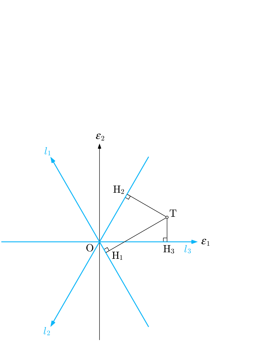
Figure 1: In the anisotropy diagram a tensor $\mbox{\boldmath$t$}=\mbox{diag}(\lambda_{1},\lambda_{2},\lambda_{3})$ is represented by a point T $=(\varepsilon_{1},\varepsilon_{2})$. The lengths of segments $(\mbox{OH}_{1},\mbox{OH}_{2},\mbox{OH}_{3})$ are equal to $\sqrt{\frac{3}{2}}(\lambda_{1},\lambda_{2},\lambda_{3})$.

Any traceless symmetric tensor can be diagonalized and parameterized in the form

$$\mbox{\boldmath$t$}=\begin{pmatrix}\lambda_{1}&0&0\\ 0&\lambda_{2}&0\\ 0&0&\lambda_{3}\end{pmatrix}=\varepsilon_{1}\frac{1}{\sqrt{6}}\begin{pmatrix}-1&0&0\\ 0&-1&0\\ 0&0&2\end{pmatrix}+\varepsilon_{2}\frac{1}{\sqrt{2}}\begin{pmatrix}1&0&0\\ 0&-1&0\\ 0&0&0\end{pmatrix}.$$ (48)

The coefficients $(\varepsilon_{1},\varepsilon_{2})$ are the same things as $(c_{5},c_{4})$ in (20) and they are related to the eigenvalues as

$$\lambda_{1}=-\frac{1}{\sqrt{6}}\,\varepsilon_{1}+\frac{1}{\sqrt{2}}\,\varepsilon_{2}=\sqrt{\frac{2}{3}}\cdot\frac{1}{2}(-1,\sqrt{3})\begin{pmatrix}\varepsilon_{1}\\ \varepsilon_{2}\end{pmatrix},$$ (49)

$$\lambda_{2}=-\frac{1}{\sqrt{6}}\,\varepsilon_{1}-\frac{1}{\sqrt{2}}\,\varepsilon_{2}=\sqrt{\frac{2}{3}}\cdot\frac{1}{2}(-1,-\sqrt{3})\begin{pmatrix}\varepsilon_{1}\\ \varepsilon_{2}\end{pmatrix},$$ (50)

$$\lambda_{3}=\sqrt{\frac{2}{3}}\,\varepsilon_{1}=\sqrt{\frac{2}{3}}\,(1,0)\begin{pmatrix}\varepsilon_{1}\\ \varepsilon_{2}\end{pmatrix},$$ (51)

or inversely

$$\varepsilon_{1}=\sqrt{\frac{3}{2}}\,\lambda_{3},$$ (52)

$$\varepsilon_{2}=\frac{1}{\sqrt{2}}(\lambda_{1}-\lambda_{2})=\frac{1}{\sqrt{2}}(2\lambda_{1}+\lambda_{3})=\frac{1}{\sqrt{2}}(-2\lambda_{2}-\lambda_{3}),$$ (53)

$$0=\lambda_{1}+\lambda_{2}+\lambda_{3}.$$ (54)

The inner product (17) is used to define the norm of the tensor

$$\alpha=||\mbox{\boldmath$t$}||=\sqrt{\langle\mbox{\boldmath$t$},\mbox{\boldmath$t$}\rangle}=\sqrt{(\lambda_{1})^{2}+(\lambda_{2})^{2}+(\lambda_{3})^{2}}=\sqrt{(\varepsilon_{1})^{2}+(\varepsilon_{2})^{2}}.$$ (55)

Then $\alpha^{2}$ is equal to the anisotropy index $3\tilde{\Delta}$ which was defined at (39). For the tensor $t$ we plot a point T whose Cartesian coordinate is $(\varepsilon_{1},\varepsilon_{2})$ as shown in Fig. 1. Thus each point in the plane defines a corresponding traceless symmetric tensor. This plane diagram is called an anisotropy diagram. The value of $\alpha$ is equal to the distance between the point T and the origin O of the coordinate.

We explain how to draw the anisotropy diagram in detail. For a given traceless tensor $t$ one calculates the eigenvalues $(\lambda_{1},\lambda_{2},\lambda_{3})$. Next one calculates $(\varepsilon_{1},\varepsilon_{2})$ using Eqs. (52), (53). Plot a point T $=(\varepsilon_{1},\varepsilon_{2})$ in the Cartesian coordinate. This is the point representing the tensor. Draw three lines $\ell_{1},\ell_{2},\ell_{3}$ which run through the origin $\rm{O}=(0,0)$ in the direction $(-\frac{1}{2},\frac{\sqrt{3}}{2})$, $(-\frac{1}{2},-\frac{\sqrt{3}}{2})$, $(1,0)$, respectively. Draw a line $m_{1}$ which runs through the point T and is perpendicular to the line $\ell_{1}$. The intersection of $\ell_{1}$ and $m_{1}$ is denoted as $\rm{H}_{1}$. Similarly, draw lines $m_{2}$ and $m_{3}$ which run through the point T and are perpendicular to the line $\ell_{2}$ and $\ell_{3}$, respectively. The intersection of $\ell_{2}$ and $m_{2}$ is denoted as $\rm{H}_{2}$. The intersection of $\ell_{3}$ and $m_{3}$ is denoted as $\rm{H}_{3}$. Then the lengths of $\rm{OH}_{1},\rm{OH}_{2},\rm{OH}_{3}$ are equal to $\sqrt{\frac{3}{2}}\,\lambda_{1},\sqrt{\frac{3}{2}}\,\lambda_{2},\sqrt{\frac{3}{2}}\,\lambda_{3}$, respectively. In this way, we can determine the set of eigenvalues from the representing point, and vice versa.

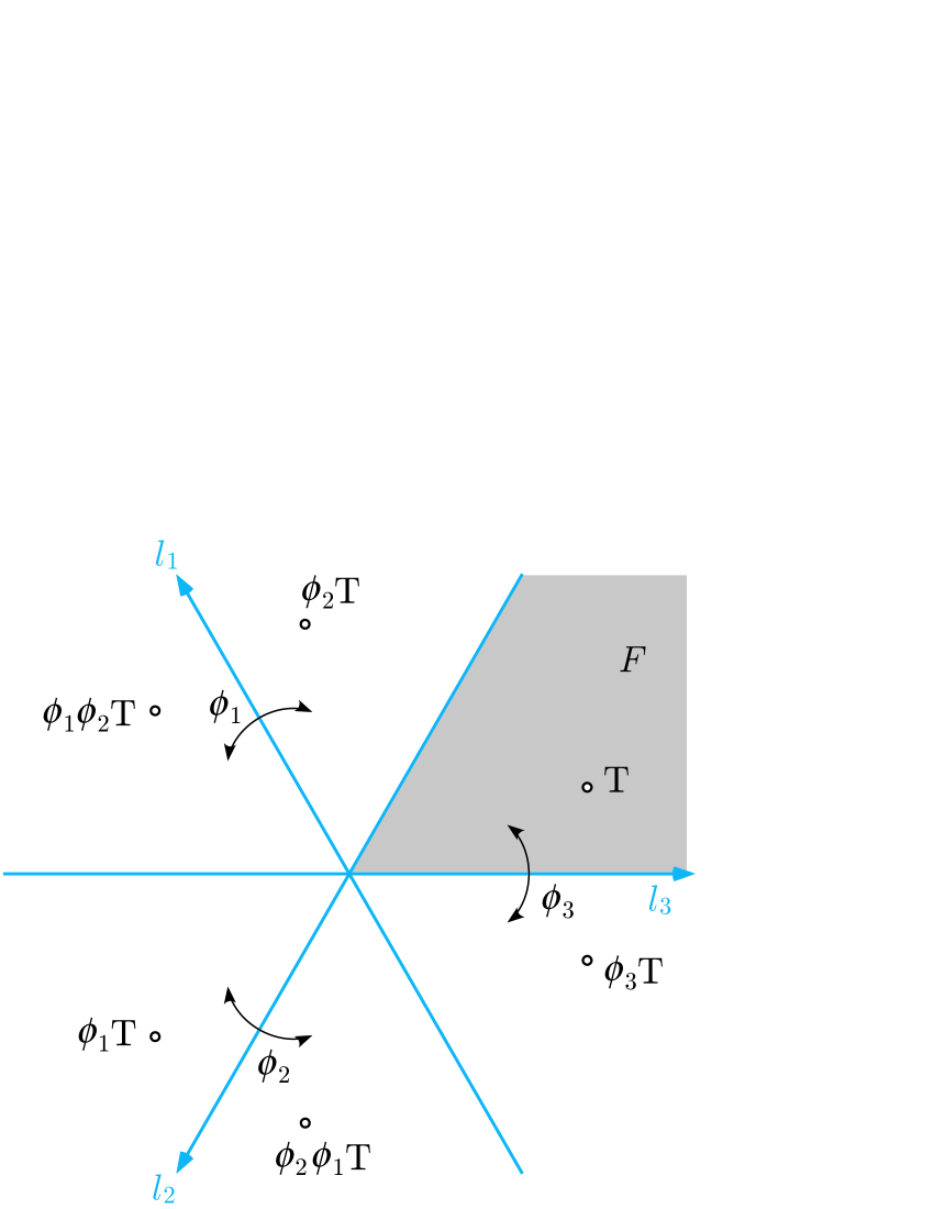
Figure 2: A permutation of the eigenvalues $\lambda_{2}\leftrightarrow\lambda_{3}$ induces the transformation $\phi_{1}$ of the anisotropy diagram, which is a reflection about the line $\ell_{1}$. Similarly, other permutations $\lambda_{3}\leftrightarrow\lambda_{1}$ and $\lambda_{1}\leftrightarrow\lambda_{2}$ induce $\phi_{2}$ and $\phi_{3}$, respectively. The permutations of the eigenvalues generate six equivalent points. There is a unique representative point in the fundamental domain $F$.

If it is not requested to arrange the eigenvalues in the order $\lambda_{3}\geq\lambda_{1}\geq\lambda_{2}$ and it is allowed to rearrange them, a point in the anisotropy diagram corresponding to the given tensor is not unique. The operation exchanging $\lambda_{2}\leftrightarrow\lambda_{3}$ induces a transformation of the coordinate of the anisotropy diagram as

$$\varepsilon^{\prime}_{1}=\sqrt{\frac{3}{2}}\,\lambda_{2}=\sqrt{\frac{3}{2}}\left(-\frac{1}{\sqrt{6}}\,\varepsilon_{1}-\frac{1}{\sqrt{2}}\,\varepsilon_{2}\right)=-\frac{1}{2}\,\varepsilon_{1}-\frac{\sqrt{3}}{2}\,\varepsilon_{2},$$

$$\varepsilon^{\prime}_{2}=\frac{1}{\sqrt{2}}(2\lambda_{1}+\lambda_{2})=\frac{1}{\sqrt{2}}\left(\frac{-3}{\sqrt{6}}\,\varepsilon_{1}+\frac{1}{\sqrt{2}}\,\varepsilon_{2}\right)=-\frac{\sqrt{3}}{2}\,\varepsilon_{1}+\frac{1}{2}\,\varepsilon_{2},$$

which can be summarized as

$$\phi_{1}:\begin{pmatrix}\varepsilon_{1}\\ \varepsilon_{2}\end{pmatrix}\mapsto\begin{pmatrix}\varepsilon_{1}^{\prime}\\ \varepsilon_{2}^{\prime}\end{pmatrix}=\frac{1}{2}\begin{pmatrix}-1&-\sqrt{3}\\ -\sqrt{3}&1\end{pmatrix}\begin{pmatrix}\varepsilon_{1}\\ \varepsilon_{2}\end{pmatrix}.$$ (56)

The permutation $\lambda_{3}\leftrightarrow\lambda_{1}$ induces a transformation

$$\varepsilon^{\prime}_{1}=\sqrt{\frac{3}{2}}\,\lambda_{1}=\sqrt{\frac{3}{2}}\left(-\frac{1}{\sqrt{6}}\,\varepsilon_{1}+\frac{1}{\sqrt{2}}\,\varepsilon_{2}\right)=-\frac{1}{2}\,\varepsilon_{1}+\frac{\sqrt{3}}{2}\,\varepsilon_{2},$$

$$\varepsilon_{2}^{\prime}=\frac{1}{\sqrt{2}}(-2\lambda_{2}-\lambda_{1})=\frac{1}{\sqrt{2}}\left(\frac{3}{\sqrt{6}}\,\varepsilon_{1}+\frac{1}{\sqrt{2}}\,\varepsilon_{2}\right)=\frac{\sqrt{3}}{2}\,\varepsilon_{1}+\frac{1}{2}\,\varepsilon_{2},$$

namely,

$$\phi_{2}:\begin{pmatrix}\varepsilon_{1}\\ \varepsilon_{2}\end{pmatrix}\mapsto\begin{pmatrix}\varepsilon_{1}^{\prime}\\ \varepsilon_{2}^{\prime}\end{pmatrix}=\frac{1}{2}\begin{pmatrix}-1&\sqrt{3}\\ \sqrt{3}&1\end{pmatrix}\begin{pmatrix}\varepsilon_{1}\\ \varepsilon_{2}\end{pmatrix}.$$ (57)

Another permutation $\lambda_{1}\leftrightarrow\lambda_{2}$ induces a transformation

$$\phi_{3}:\begin{pmatrix}\varepsilon_{1}\\ \varepsilon_{2}\end{pmatrix}\mapsto\begin{pmatrix}\varepsilon^{\prime}_{1}\\ \varepsilon^{\prime}_{2}\end{pmatrix}=\begin{pmatrix}1&0\\ 0&-1\end{pmatrix}\begin{pmatrix}\varepsilon_{1}\\ \varepsilon_{2}\end{pmatrix}.$$ (58)

A point T is moved to the point $\phi_{1}{\rm T}$ by the mapping $\phi_{1}$. Furthermore, it can be moved to the point $\phi_{2}\phi_{1}{\rm T}$ by $\phi_{2}$, and so on. In the anisotropy diagram Fig. 2, the transformations $\phi_{1},\phi_{2},\phi_{3}$ are reflections with respect to the lines $\ell_{1},\ell_{2},\ell_{3}$, respectively. The set of transformations $\{\phi_{1},\phi_{2},\phi_{3}\}$ generates the third permutation group ${\mathfrak{S}}_{3}$, which has $3!=6$ elements. Under the actions of ${\mathfrak{S}}_{3}$ a generic point T in the anisotropy diagram leaves six points on its trajectory. These trajectory points $\rm{T}_{1},\cdots,\rm{T}_{6}$ are equivalent as a representative of the tensor $t$. If we impose the condition $\lambda_{3}\geq\lambda_{1}$, Eqs. (49) and (51) imply $\sqrt{3}\,\varepsilon_{1}\geq\varepsilon_{2}$. Moreover, if we impose the condition $\lambda_{1}\geq\lambda_{2}$, Eq. (53) implies $\varepsilon_{2}\geq 0$. Hence, if the eigenvalues are arranged to satisfy the conventional ordering $\lambda_{3}\geq\lambda_{1}\geq\lambda_{2}$, a unique representative point is chosen in the domain

$$F=\{(\varepsilon_{1},\varepsilon_{2})\,|\,0\leq\varepsilon_{2}\leq\sqrt{3}\,\varepsilon_{1}\},$$ (59)

which we call the fundamental domain of the anisotropy diagram.

We can use the radius $\alpha$ and an angle $\gamma$ to parameterize the coordinate of the anisotropy diagram as

$$\varepsilon_{1}=\alpha\cos\gamma,\qquad\varepsilon_{2}=\alpha\sin\gamma.$$ (60)

By substituting these variables into (49)-(51) and (41), we obtain an expression for the index of biaxiality

$$\kappa=\frac{1}{2}\Big{[}\varepsilon_{2}\,\big{\{}3(\varepsilon_{1})^{2}-(\varepsilon_{2})^{2}\big{\}}\Big{]}^{2}=\frac{1}{2}\,\alpha^{6}\sin^{2}\gamma\,(3-4\sin^{2}\gamma)^{2}.$$ (61)

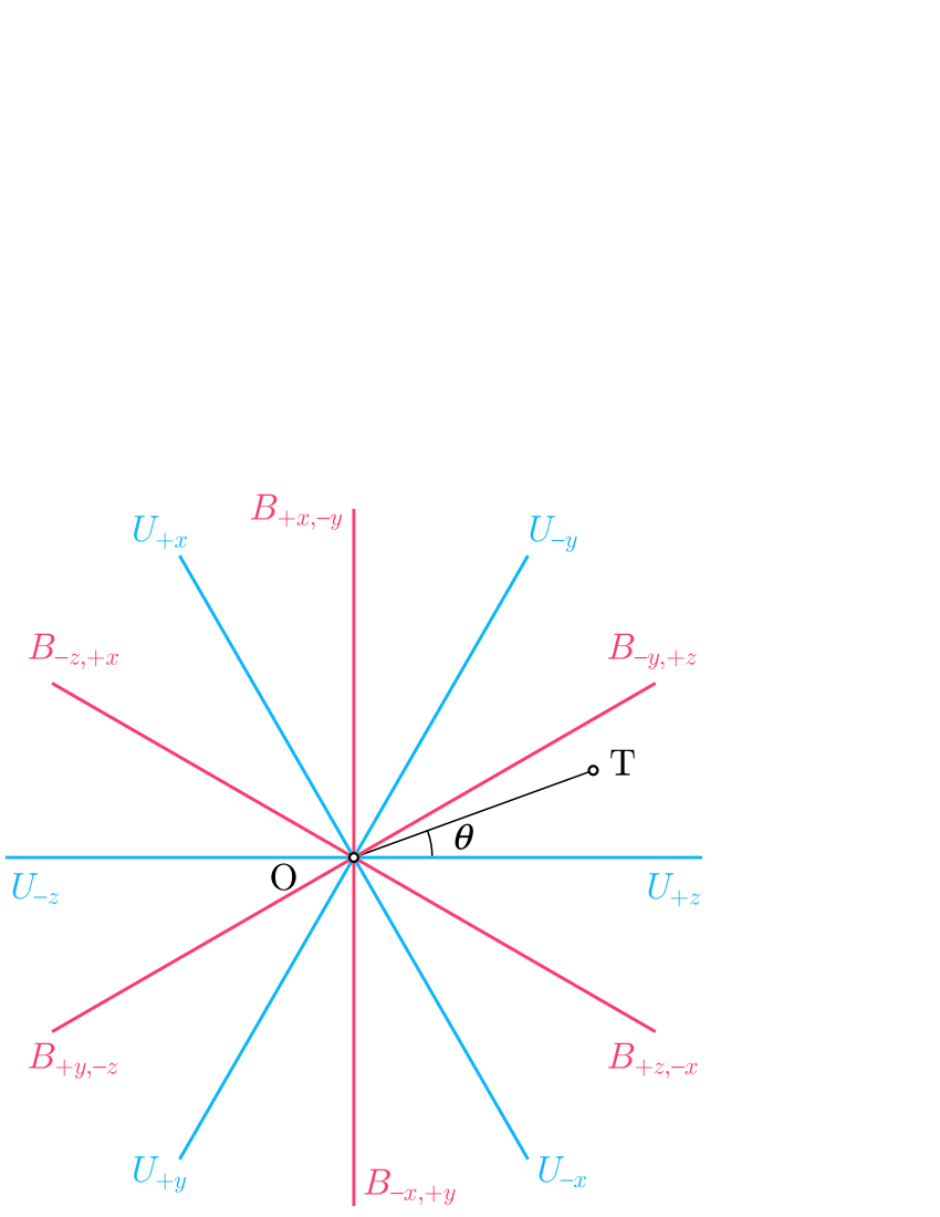
Figure 3: The half lines $\{U_{j}\}$ are uniaxial lines while the half lines $\{B_{k}\}$ are maximally biaxial lines. The degree of the anisotropy of the tensor $t$ is $\alpha=$ the length of the segment OT. The degree of the biaxiality is $\beta=\frac{6}{\pi}\theta$.

If the angle $\gamma$ is varied, $\kappa$ takes the maximum value $\frac{1}{2}\alpha^{6}$ when $\sin^{2}\gamma=\frac{1}{4}$ or 1. Hence the biaxiality becomes the maximum at $\gamma=\frac{\pi}{6},\frac{\pi}{2},\frac{5\pi}{6},\frac{7\pi}{6},\frac{3\pi}{2},\frac{11\pi}{6}$. On the other hand, $\kappa$ takes the minimum value $0$ when $\sin^{2}\gamma=0$ or $\frac{3}{4}$. Hence the biaxiality vanishes at $\gamma=0,\frac{\pi}{3},\frac{2\pi}{3},\pi,\frac{4\pi}{3},\frac{5\pi}{3}$. In the anisotropy diagram Fig. 3, we introduce a family of half lines

$$\left\{\begin{array}[]{l}U_{+x}=\{(\varepsilon_{1},\varepsilon_{2})=\frac{1}{2}r(-1,\sqrt{3})\,|\,r>0\},\\ \\ U_{-x}=\{(\varepsilon_{1},\varepsilon_{2})=-\frac{1}{2}r(-1,\sqrt{3})\,|\,r>0\},\\ \\ U_{+y}=\{(\varepsilon_{1},\varepsilon_{2})=\frac{1}{2}r(-1,-\sqrt{3})\,|\,r>0\},\\ \\ U_{-y}=\{(\varepsilon_{1},\varepsilon_{2})=-\frac{1}{2}r(-1,-\sqrt{3})\,|\,r>0\},\\ \\ U_{+z}=\{(\varepsilon_{1},\varepsilon_{2})=r(1,0)\,|\,r>0\},\\ \\ U_{-z}=\{(\varepsilon_{1},\varepsilon_{2})=-r(1,0)\,|\,r>0\}.\end{array}\right.$$ (62)

These lines divide the anisotropy diagram into six domains. Tensors which belong to $U_{\pm x},U_{\pm y},U_{\pm z}$ are

$$\pm\frac{r}{\sqrt{6}}\begin{pmatrix}2&0&0\\ 0&-1&0\\ 0&0&-1\end{pmatrix},\qquad\pm\frac{r}{\sqrt{6}}\begin{pmatrix}-1&0&0\\ 0&2&0\\ 0&0&-1\end{pmatrix},\qquad\pm\frac{r}{\sqrt{6}}\begin{pmatrix}-1&0&0\\ 0&-1&0\\ 0&0&2\end{pmatrix},$$ (63)

respectively. The half lines $\{U_{j}\}$ are called the uniaxial lines. Similarly, we introduce another family of half lines

$$\left\{\begin{array}[]{l}B_{+x,-y}=\{(\varepsilon_{1},\varepsilon_{2})=r(0,1)\,|\,r>0\},\\ \\ B_{-x,+y}=\{(\varepsilon_{1},\varepsilon_{2})=-r(0,1)\,|\,r>0\},\\ \\ B_{+y,-z}=\{(\varepsilon_{1},\varepsilon_{2})=\frac{1}{2}r(-\sqrt{3},-1)\,|\,r>0\},\\ \\ B_{-y,+z}=\{(\varepsilon_{1},\varepsilon_{2})=-\frac{1}{2}r(-\sqrt{3},-1)\,|\,r>0\},\\ \\ B_{+z,-x}=\{(\varepsilon_{1},\varepsilon_{2})=\frac{1}{2}r(\sqrt{3},-1)\,|\,r>0\},\\ \\ B_{-z,+x}=\{(\varepsilon_{1},\varepsilon_{2})=-\frac{1}{2}r(\sqrt{3},-1)\,|\,r>0\}.\end{array}\right.$$ (64)

Then tensors which belong to $B_{\pm x,\mp y},B_{\pm y,\mp z},B_{\pm z,\mp x}$ are

$$\pm\frac{r}{\sqrt{2}}\begin{pmatrix}1&0&0\\ 0&-1&0\\ 0&0&0\end{pmatrix},\qquad\pm\frac{r}{\sqrt{2}}\begin{pmatrix}0&0&0\\ 0&1&0\\ 0&0&-1\end{pmatrix},\qquad\pm\frac{r}{\sqrt{2}}\begin{pmatrix}-1&0&0\\ 0&0&0\\ 0&0&1\end{pmatrix}.$$ (65)

The half lines $\{B_{k}\}$ are called the maximally biaxial lines.

Using the anisotropy diagram we can classify tensors and measure their degrees of anisotropy. An isotropic tensor is represented by the origin of the diagram. A uniaxial tensor is represented by three equivalent points on the uniaxial lines. A biaxial tensor is represented by six equivalent points and each point belongs to one of the six domains divided by the uniaxial lines. As shown in Fig. 3, a generic point T in the diagram is sandwiched between one of uniaxial half lines and one of maximally biaxial half lines, which are denoted as $U_{j}$ and $B_{k}$. The degree of anisotropy is measured by the radius OT $=\alpha$ defined at (55). The angle between $U_{j}$ and $B_{k}$ is $(\pi/6)$ rad. Let $\theta$ be the magnitude of the angle formed by the half lines OT and $U_{j}$ measured in radians. Then we can define the degree of biaxiality $\beta$ by

$$\beta=\frac{6}{\pi}\,\theta.$$ (66)

Then $\beta$ takes its value in the range $0\leq\beta\leq 1$. Bates and Luckhurst [24] gave another definition of biaxiality index $\eta$, which they called the relative biaxiality,

$$\eta=\frac{\lambda_{1}-\lambda_{2}}{\lambda_{3}}$$ (67)

for $\lambda_{3}\geq 0\geq\lambda_{1}\geq\lambda_{2}$. It is equal to

$$\eta=\sqrt{3}\;\frac{\varepsilon_{2}}{\varepsilon_{1}}=\sqrt{3}\,\tan\theta=\frac{\tan\theta}{\tan(\pi/6)}.$$ (68)

The index $\eta$ is a monotonically increasing function of $\beta$ and it also takes its value in the range $0\leq\eta\leq 1$. The intuitive meaning of $\eta$ is also clear. As another index of biaxiality we may define

$$\zeta=\frac{2\,\kappa}{\alpha^{6}}\,.$$ (69)

The index $\zeta$ also takes its value in $0\leq\zeta\leq 1$ since the value of $\kappa$ is within $0\leq\kappa\leq\frac{1}{2}\alpha^{6}$ as discussed at (61).

Here we need to mention that diagrams which are similar to our anisotropic diagram can be found in literatures. Kralj, Virga, and Žumer [18] introduced a diagram which is equivalent to the anisotropic diagram. A new point of our study is that we use the diagram as a tool for comparing various tensorial quantities and for measuring the degrees of anisotropies. Another new point is that we establish a relation between the microscopic quantity and the macroscopic quantity in the anisotropic diagram as will be discussed in the next section. For a comparison with Kralj’s parameterization, Eq. (9) in their paper [18], we write the eigenvalues (49)-(51) in terms of the variables (60) as

$$\lambda_{1}=\sqrt{\frac{2}{3}}\,\alpha\,\cos\Big{(}\gamma-\frac{2\pi}{3}\Big{)},\quad\lambda_{2}=\sqrt{\frac{2}{3}}\,\alpha\,\cos\Big{(}\gamma+\frac{2\pi}{3}\Big{)},\quad\lambda_{3}=\sqrt{\frac{2}{3}}\,\alpha\,\cos\gamma.$$ (70)

5 Micro-macro relation

In the previous section we introduced the anisotropy diagram, the degree of anisotropy $\alpha$, and the degree of biaxiality $\beta$. We have introduced also the geometric order parameter $G$ which connects the microscopic tensorial quantity $t$ with the macroscopic tensorial quantity $\langle\tilde{\mbox{\boldmath$t$}}\rangle=G\mbox{\boldmath$t$}$. In this section we will discuss how the degrees of anisotropy of the macroscopic quantity is related to the degrees of anisotropy of the microscopic quantity. We will establish a diagrammatic relation between them, which we call the micro-macro relation.

The idea of the micro-macro relation was inspired by Ojima’s idea, Micro-macro duality [27]. Micro-macro duality means bi-directional relations between the microscopic quantum world and the macroscopic classical world. Although our present consideration is restricted within classical physics, the relation between the molecular quantity and the macroscopic quantity can be regarded as an example of Micro-macro duality.

Let us confirm notation to be used below. The orientation of a molecule in liquid crystal is described by a three-dimensional rotation matrix $R\in SO(3)$. The molecules have various orientations and their statistical distribution is described by the probability density $p(R)$. Assume that each molecule has a physical quantity which is represented by a traceless symmetric tensor $t$. When a molecule is turned by a matrix $R$, the tensor is transformed to $(R\otimes R)\mbox{\boldmath$t$}=R\,\mbox{\boldmath$t$}\,R^{T}$. Then the average

$$\langle\tilde{\mbox{\boldmath$t$}}\rangle=\int(R\otimes R)\mbox{\boldmath$t$}\,p(R)\,dR=\int(R\,\mbox{\boldmath$t$}\,R^{T})\,p(R)\,dR=G\mbox{\boldmath$t$}$$ (71)

Figure 4: The points $\{{\rm T}_{1},\cdots,{\rm T}_{6}\}$ are equivalent points representing a tensor $t$. The point $\tilde{\rm T}$ represents the average tensor $\langle\tilde{\mbox{\boldmath$t$}}\rangle$. The point $\tilde{\rm T}$ is always in the polygon $D$ whose vertices are $\{{\rm T}_{1},\cdots,{\rm T}_{6}\}$. (a) T is uniaxial. (b) T is generic. (c) T is maximally biaxial.

is the quantity observed at the macroscopic scale. The tensor $R\,\mbox{\boldmath$t$}\,{R}^{T}$ has the same set of eigenvalues as $t$ for any rotation matrix $R$. However, in general, the principal axes of ${R^{\prime}}\,\mbox{\boldmath$t$}\,{R^{\prime}}^{T}$ do not coincide with those of $R\,\mbox{\boldmath$t$}\,R^{T}$ for different matrices $R$ and $R^{\prime}$. In other words, the matrices $\{R\,\mbox{\boldmath$t$}\,R^{T}\}$ defined with various $R\in SO(3)$ are not simultaneously diagonalizable. Hence, it seems nontrivial to find a general relation which holds between the eigenvalues of $t$ and those of $\langle\tilde{\mbox{\boldmath$t$}}\rangle$. This is actually what we found and is called the micro-macro relation.

Let $\{\rm{T}_{1},\cdots,\rm{T}_{6}\}$ be the set of equivalent points in the anisotropy diagram which corresponds to the tensor $t$. The degrees of anisotropy and biaxiality of $t$ are written as $\alpha(\mbox{\boldmath$t$})$ and $\beta(\mbox{\boldmath$t$})$, respectively. Let $\tilde{\rm{T}}$ be a point in the anisotropy diagram Fig. 4 which corresponds to $\langle\tilde{\mbox{\boldmath$t$}}\rangle$. Let $D$ be a convex polygon which has the points $\{\rm{T}_{1},\cdots,\rm{T}_{6}\}$ as its vertices. Both the perimeter and the inner domain of $D$ are included in $D$. Let P be an arbitrary point of $D$. Then the following two theorems hold.
Theorem 1. For any probability distribution $p(R)$, the average point $\tilde{T}$ is in the polygon $D$.
Theorem 2. For any point P in $D$, there exists a probability distribution $p(R)$ such that the average point $\tilde{T}$ coincides with the point P.

Before showing proofs of these theorems, we introduce three kinds of indices which enable us to compare anisotropies of microscopic and macroscopic quantities. We call the ratio of the degrees of anisotropy

$$\chi_{1}=\frac{\alpha(\langle\tilde{\mbox{\boldmath$t$}}\rangle)}{\alpha(\mbox{\boldmath$t$})}$$ (72)

the strength of realization of anisotropy. Theorem 1 implies that the length of the segment ${\rm O}\tilde{\rm T}$ cannot be longer than the length of OT. By definition, ${\rm O}\tilde{\rm T}=\alpha(\langle\tilde{\mbox{\boldmath$t$}}\rangle)$ and OT $=\alpha(\mbox{\boldmath$t$})$. Hence, their ratio $\chi_{1}$ is in the range $0\leq\chi_{1}\leq 1$. In particular, for the pair of the microscopic singular tensor $\mbox{\boldmath$t$}_{\alpha}$ and the macroscopic singular tensor $\mbox{\boldmath$u$}_{\alpha}$ which satisfies Eq. (31), the strength of realization of anisotropy $\chi_{1}$ is equal to the degree of order $\sigma_{\alpha}$.

We call the ratio of the degrees of biaxiality

$$\chi_{2}=\frac{\beta(\langle\tilde{\mbox{\boldmath$t$}}\rangle)}{\beta(\mbox{\boldmath$t$})}$$ (73)

the strength of realization of biaxiality. The value of $\chi_{2}$ can be larger than 1. In such a case it is said that biaxiality is enhanced in the macroscopic phase. It can happen that $\beta(\langle\tilde{\mbox{\boldmath$t$}}\rangle)\neq 0$ even when $\beta(\mbox{\boldmath$t$})=0$. In such a case we formally write $\chi_{2}=\infty$ and say that biaxiality is generated from uniaxial molecules. Conversely, it also can happen that $\beta(\langle\tilde{\mbox{\boldmath$t$}}\rangle)=0$ although $\beta(\mbox{\boldmath$t$})\neq 0$. In such a case we have $\chi_{2}=0$ and say that biaxiality is lost or uniaxiality is realized from biaxial molecules in the macroscopic phase.

We define the third index

$$\chi_{3}=\mbox{sgn}\,(\det\langle\tilde{\mbox{\boldmath$t$}}\rangle\,\det\mbox{\boldmath$t$}),$$ (74)

and call it the relative signature. Here sgn $(x)$ denotes the signature of $x$ and it takes its value in $\{1,0,-1\}$. When $\chi_{3}=1$, we say that the macroscopic phase is positively oriented or it has prolate order. When $\chi_{3}=-1$, we say that the macroscopic phase is negatively oriented or it has oblate order.

We would like to show another theorem. Theorem 1 is a corollary of this theorem:
Theorem 3. Let $\lambda_{\tiny\rm max}$ and $\lambda_{\tiny\rm min}$ be the maximum and the minimum, respectively, among the eigenvalues $\{\lambda_{1},\lambda_{2},\lambda_{3}\}$ of $t$. Let $\{\mu_{1},\mu_{2},\mu_{3}\}$ be the eigenvalues of $\langle\tilde{\mbox{\boldmath$t$}}\rangle$. Then, it holds that

$$\lambda_{\tiny\rm min}\leq\mu_{r}\leq\lambda_{\tiny\rm max},\qquad r=1,2,3.$$ (75)

Proof of theorem 3: Let $\mbox{\boldmath$v$}_{r}$ be a normalized eigenvector satisfying $\langle\tilde{\mbox{\boldmath$t$}}\rangle\mbox{\boldmath$v$}_{r}=\mu_{r}\mbox{\boldmath$v$}_{r}$. This equation is to be read as a multiplication of the matrix $\langle\tilde{\mbox{\boldmath$t$}}\rangle$ on the vector $\mbox{\boldmath$v$}_{r}$ as

$$\sum_{j=1}^{3}\>\langle\tilde{t}_{ij}\rangle(v_{r})_{j}=\mu_{r}(v_{r})_{i}.$$ (76)

We write an inner product of vectors $v$ and $w$ as $\langle\mbox{\boldmath$v$},\mbox{\boldmath$w$}\rangle=\sum_{i=1}^{3}v_{i}\,w_{i}$. Then we have

$$\mu_{r} = \mu_{r}\langle\mbox{\boldmath$v$}_{r},\mbox{\boldmath$v$}_{r}\rangle$$ (77)

$$= \langle\mbox{\boldmath$v$}_{r},\langle\tilde{\mbox{\boldmath$t$}}\rangle\mbox{\boldmath$v$}_{r}\rangle$$

$$= \Big{\langle}\mbox{\boldmath$v$}_{r},\int(R\,\mbox{\boldmath$t$}\,R^{T})\,p(R)\,dR\,\mbox{\boldmath$v$}_{r}\Big{\rangle}$$

$$= \int\langle R^{T}\mbox{\boldmath$v$}_{r},\mbox{\boldmath$t$}\,R^{T}\mbox{\boldmath$v$}_{r}\rangle\,p(R)\,dR$$

$$= \int\mbox{Tr}\Big{\{}\mbox{\boldmath$t$}\,(R^{T}\mbox{\boldmath$v$}_{r}\otimes R^{T}\mbox{\boldmath$v$}_{r})\Big{\}}\,p(R)\,dR$$

$$= \mbox{Tr}\Big{\{}\mbox{\boldmath$t$}\int(R^{T}\mbox{\boldmath$v$}_{r}\otimes R^{T}\mbox{\boldmath$v$}_{r})\,p(R)\,dR\Big{\}}$$

$$= \mbox{Tr}(\mbox{\boldmath$t$}\,\rho_{r}).$$

In the last line we introduced the three-dimensional matrix $\rho_{r}$ which is defined by

$$\rho_{r}=\int(R^{T}\mbox{\boldmath$v$}_{r}\otimes R^{T}\mbox{\boldmath$v$}_{r})\,p(R)\,dR=\int R^{T}(\mbox{\boldmath$v$}_{r}\otimes\mbox{\boldmath$v$}_{r})R\,p(R)\,dR.$$ (78)

The matrix $\rho_{r}$ is symmetric, non-negative and satisfies $\mbox{Tr}\,\rho_{r}=1$. On the other hand, let

$$\mbox{\boldmath$t$}=\lambda_{1}\Pi_{1}+\lambda_{2}\Pi_{2}+\lambda_{3}\Pi_{3}$$ (79)

be the spectral decomposition of $t$. The three-dimensional matrices $\{\Pi_{q}\}$ satisfy $(\Pi_{q})^{T}=\Pi_{q}$, $\Pi_{q}\Pi_{s}=\delta_{qs}\Pi_{s}$, $\sum_{q=1}^{3}\Pi_{q}=I$, $\mbox{Tr}\,\Pi_{q}=1$. Substituting this into (77) we obtain

$$\mu_{r}=\mbox{Tr}(\rho_{r}\,\mbox{\boldmath$t$})=\sum_{q=1}^{3}\mbox{Tr}(\rho_{r}\Pi_{q})\,\lambda_{q}=\sum_{q=1}^{3}P_{rq}\,\lambda_{q}$$ (80)

where $P_{rq}=\mbox{Tr}(\rho_{r}\Pi_{q})$ are non-negative real numbers and satisfy $\sum_{q=1}^{3}P_{rq}=1$. Hence,

$$\mu_{r}=\sum_{q=1}^{3}P_{rq}\,\lambda_{q}\;\leq\;\sum_{q=1}^{3}P_{rq}\,\lambda_{\tiny\rm max}=\lambda_{\tiny\rm max},$$ (81)

$$\mu_{r}=\sum_{q=1}^{3}P_{rq}\,\lambda_{q}\;\geq\;\sum_{q=1}^{3}P_{rq}\,\lambda_{\tiny\rm min}=\lambda_{\tiny\rm min}.$$ (82)

This ends the proof of theorem 3. It is also interesting to note that $\sum_{r=1}^{3}\rho_{r}=I$ and therefore $\sum_{r=1}^{3}P_{rq}=1$.

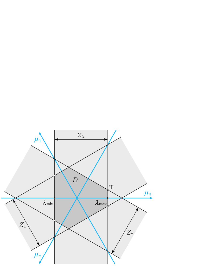
Figure 5: The intersection of the shaded bands, $Z_{1},Z_{2},Z_{3}$ defines the polygon $D$. The average point is restricted in $D$.

Proof of theorem 1: From the construction of the anisotropy diagram it is obvious that the set of points satisfying the inequality (75) is the polygon $D$. See the Fig. 5. This fact can be also verified via explicit calculations. The coordinate $(\tilde{\varepsilon}_{1},\tilde{\varepsilon}_{2})$ of the point $\tilde{\rm{T}}$ is defined by

$$\tilde{\varepsilon}_{1}=\sqrt{\frac{3}{2}}\,\mu_{3},\qquad\tilde{\varepsilon}_{2}=\frac{1}{\sqrt{2}}(\mu_{1}-\mu_{2}).$$ (83)

They satisfy the equation similar to (49)-(51),

$$\mu_{1}=-\frac{1}{\sqrt{6}}\,\tilde{\varepsilon}_{1}+\frac{1}{\sqrt{2}}\,\tilde{\varepsilon}_{2}=\sqrt{\frac{2}{3}}\cdot\frac{1}{2}(-1,\sqrt{3})\begin{pmatrix}\tilde{\varepsilon}_{1}\\ \tilde{\varepsilon}_{2}\end{pmatrix},$$ (84)

$$\mu_{2}=-\frac{1}{\sqrt{6}}\,\tilde{\varepsilon}_{1}-\frac{1}{\sqrt{2}}\,\tilde{\varepsilon}_{2}=\sqrt{\frac{2}{3}}\cdot\frac{1}{2}(-1,-\sqrt{3})\begin{pmatrix}\tilde{\varepsilon}_{1}\\ \tilde{\varepsilon}_{2}\end{pmatrix},$$ (85)

$$\mu_{3}=\sqrt{\frac{2}{3}}\,\tilde{\varepsilon}_{1}=\sqrt{\frac{2}{3}}\,(1,0)\begin{pmatrix}\tilde{\varepsilon}_{1}\\ \tilde{\varepsilon}_{2}\end{pmatrix}.$$ (86)

Hence the sets of points restricted by the inequality (75),

$$Z_{1}=\{(\tilde{\varepsilon}_{1},\tilde{\varepsilon}_{2})\,|\,\lambda_{\tiny\rm min}\leq-\frac{1}{\sqrt{6}}\,\tilde{\varepsilon}_{1}+\frac{1}{\sqrt{2}}\,\tilde{\varepsilon}_{2}\leq\lambda_{\tiny\rm max}\},$$ (87)

$$Z_{2}=\{(\tilde{\varepsilon}_{1},\tilde{\varepsilon}_{2})\,|\,\lambda_{\tiny\rm min}\leq-\frac{1}{\sqrt{6}}\,\tilde{\varepsilon}_{1}-\frac{1}{\sqrt{2}}\,\tilde{\varepsilon}_{2}\leq\lambda_{\tiny\rm max}\},$$ (88)

$$Z_{3}=\{(\tilde{\varepsilon}_{1},\tilde{\varepsilon}_{2})\,|\,\lambda_{\tiny\rm min}\leq\sqrt{\frac{2}{3}}\,\tilde{\varepsilon}_{1}\leq\lambda_{\tiny\rm max}\},$$ (89)

are drawn as three shaded bands in Fig. 5. Their intersection $Z_{1}\cap Z_{2}\cap Z_{3}$ is nothing but the polygon $D$. This observation proves theorem 1.

Proof of theorem 2: First, let us note the following simple fact. Suppose that two traceless symmetric tensors $\mbox{\boldmath$t$}_{0}$ and $\mbox{\boldmath$t$}_{1}$ are simultaneously diagonalizable. In other words, they have common principal axes. Let $\rm{T}_{0}$ and $\rm{T}_{1}$ be their representing points in the anisotropy diagram. Then the weighted sum

$$\mbox{\boldmath$t$}_{w}=(1-w)\mbox{\boldmath$t$}_{0}+w\mbox{\boldmath$t$}_{1}$$ (90)

with a real number $w$ $(0\leq w\leq 1)$ is also a traceless symmetric tensor and diagonalizable simultaneously with $\mbox{\boldmath$t$}_{0}$ and $\mbox{\boldmath$t$}_{1}$. It is easily verified that the point ${\rm T}_{w}$ representing $\mbox{\boldmath$t$}_{w}$ in the anisotropy diagram divides the segment $\rm{T}_{0}\rm{T}_{1}$ in the ratio $w:(1-w)$.

Second, let us note that any point P of a convex polygon can be expressed as a weighted sum of the vertices of the polygon. We can chose real numbers $w_{1},\cdots,w_{6}$ such that

$$\mbox{\boldmath$t$}_{\rm P}=\sum_{i=1}^{6}w_{i}\mbox{\boldmath$t$}_{i},\qquad\sum_{i=1}^{6}w_{i}=1,\qquad 0\leq w_{i}\leq 1$$ (91)

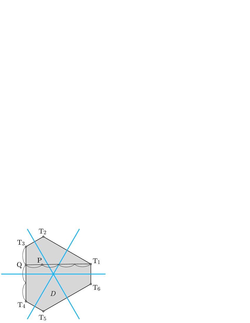
Figure 6: The point Q divides the edge ${\rm T}_{3}{\rm T}_{4}$ into the ratio $1:2$. The point P divides the segment ${\rm T}_{1}{\rm Q}$ into the ratio $3:1$. Thus, Q $=\frac{2}{3}{\rm T}_{3}+\frac{1}{3}{\rm T}_{4}$, P $=\frac{1}{4}{\rm T}_{1}+\frac{3}{4}{\rm Q}=\frac{1}{4}{\rm T}_{1}+\frac{1}{2}{\rm T}_{3}+\frac{1}{4}{\rm T}_{4}$. Every point in the polygon $D$ can be expressed as a weight sum of the vertices.

For example, the point Q in Fig. 6 is given by

$$\mbox{\boldmath$t$}_{\rm Q}=\frac{2}{3}\mbox{\boldmath$t$}_{3}+\frac{1}{3}\mbox{\boldmath$t$}_{4}$$ (92)

and the point P is given by

$$\mbox{\boldmath$t$}_{\rm P}=\frac{1}{4}\mbox{\boldmath$t$}_{1}+\frac{3}{4}\mbox{\boldmath$t$}_{\rm Q}=\frac{1}{4}\mbox{\boldmath$t$}_{1}+\frac{1}{2}\mbox{\boldmath$t$}_{3}+\frac{1}{4}\mbox{\boldmath$t$}_{4}.$$ (93)

For a given point P the set of weights $(w_{1},\cdots,w_{6})$ is not unique but uniqueness is not necessary.

Third, remember that the vertices of the polygon $D$ in the anisotropy diagram are related to each other by reflections $\phi_{1},\phi_{2},\phi_{3}$. Note that these reflections in the diagram can be generated by rotations in the real space. If we define

$$K_{1}=\begin{pmatrix}1&0&0\\ 0&0&-1\\ 0&1&0\end{pmatrix},\qquad K_{2}=\begin{pmatrix}0&0&1\\ 0&1&0\\ -1&0&0\end{pmatrix},\qquad K_{3}=\begin{pmatrix}0&-1&0\\ 1&0&0\\ 0&0&1\end{pmatrix},$$ (94)

then the reflection mapping $\phi_{i}$ introduced in Sec. 4 is equivalent to the rotation $\phi_{i}\mbox{\boldmath$t$}=K_{i}\,\mbox{\boldmath$t$}\,K_{i}^{T}$. Hence, for the vertices $\mbox{\boldmath$t$}_{1}(=\mbox{\boldmath$t$}),\mbox{\boldmath$t$}_{2},\cdots,\mbox{\boldmath$t$}_{6}$ of the polygon there exists a set of rotation matrices $R_{1},$ $R_{2},\cdots,$ $R_{6}$ such that $\mbox{\boldmath$t$}_{i}=R_{i}\,\mbox{\boldmath$t$}\,R_{i}^{T}$.

Finally, combining the above arguments we obtain

$$\mbox{\boldmath$t$}_{\rm P}=\sum_{i=1}^{6}w_{i}\mbox{\boldmath$t$}_{i}=\sum_{i=1}^{6}w_{i}(R_{i}\,\mbox{\boldmath$t$}\,R_{i}^{T}),$$ (95)

which should be compared with Eq. (71). This means that the set of weights $(w_{1},\cdots,w_{6})$ is a probability distribution which yields the point P as the average. This proves theorem 2.

The collection of theorem 1, 2, and 3 is called the micro-macro relation.

6 Examples

In this section we will demonstrate calculations of the macroscopic tensors by assuming simple probability distributions. In the first example we will show that uniaxial molecules can generate a biaxial order at the macroscopic scale. In the second example we will show that uniaxial molecules can exhibit a negatively oriented uniaxial phase. The third example has a continuous probability distribution and will exhibit the same result as the second one. In the fourth example we will show that biaxial molecules can exhibit a uniaxial order.

In the first example we assume that the molecule has a physical quantity

$$\mbox{\boldmath$t$}=\frac{1}{\sqrt{6}}\begin{pmatrix}-1&0&0\\ 0&-1&0\\ 0&0&2\end{pmatrix},$$ (96)

which has positive uniaxiality on the $z$-axis. The anisotropy diagram for this is shown in Fig. 7 (a). The coordinate of the representing point T is $(\varepsilon_{1},\varepsilon_{2})=(1,0)$. Assume that 2/3 of molecules are aligned in the $z$-direction and 1/3 of molecules turn into the $x$-direction. Then the average of the tensorial quantity is

$$\langle\tilde{\mbox{\boldmath$t$}}\rangle_{1}=\frac{2}{3}\mbox{\boldmath$t$}+\frac{1}{3}(K_{2}\mbox{\boldmath$t$}K_{2}^{T}) = \frac{2}{3}\cdot\frac{1}{\sqrt{6}}\begin{pmatrix}-1&0&0\\ 0&-1&0\\ 0&0&2\end{pmatrix}+\frac{1}{3}\cdot\frac{1}{\sqrt{6}}\begin{pmatrix}2&0&0\\ 0&-1&0\\ 0&0&-1\end{pmatrix}$$ (97)

$$= \frac{1}{\sqrt{6}}\begin{pmatrix}0&0&0\\ 0&-1&0\\ 0&0&1\end{pmatrix}.$$

The coordinate of the point $\tilde{\rm T}_{1}$ corresponding to $\langle\tilde{\mbox{\boldmath$t$}}\rangle_{1}$ is $(\tilde{\varepsilon}_{1},\tilde{\varepsilon}_{2})=\frac{1}{2}(1,\frac{1}{\sqrt{3}})$ and it lies on the half line $B_{-y,+z}$. The maximal biaxiality is realized in this case. The strength of realization of anisotropy is

$$\chi_{1}=\frac{\alpha(\langle\tilde{\mbox{\boldmath$t$}}\rangle_{1})}{\alpha(\mbox{\boldmath$t$})}=\sqrt{\frac{2}{6}}=\frac{1}{\sqrt{3}}.$$ (98)

The degrees of biaxiality are $\beta(\mbox{\boldmath$t$})=0$ and $\beta(\langle\tilde{\mbox{\boldmath$t$}}\rangle_{1})=1$. Hence the strength of realization of biaxiality is $\chi_{2}=\infty$.

Next, assume that 1/2 of molecules turn in the $x$-direction and 1/2 of molecules turn into the $y$-direction. Then the average is

$$\langle\tilde{\mbox{\boldmath$t$}}\rangle_{2}=\frac{1}{2}(K_{2}\mbox{\boldmath$t$}K_{2}^{T})+\frac{1}{2}(K_{1}\mbox{\boldmath$t$}K_{1}^{T}) = \frac{1}{2}\cdot\frac{1}{\sqrt{6}}\begin{pmatrix}2&0&0\\ 0&-1&0\\ 0&0&-1\end{pmatrix}+\frac{1}{2}\cdot\frac{1}{\sqrt{6}}\begin{pmatrix}-1&0&0\\ 0&2&0\\ 0&0&-1\end{pmatrix}$$ (99)

$$= \frac{1}{2\sqrt{6}}\begin{pmatrix}1&0&0\\ 0&1&0\\ 0&0&-2\end{pmatrix}.$$

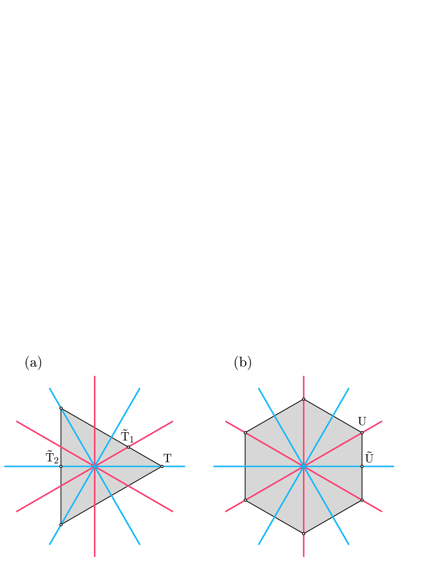
Figure 7: Examples of calculation of the average tensor $\tilde{\rm T}$ from the microscopic tensor T. (a) The uniaxial tensor T can generate the biaxial $\tilde{\rm T}_{1}$. It can also generate the uniaxial $\tilde{\rm T}_{2}$ with the inverted signature. (b) The biaxial tensor U can generate the uniaxial $\tilde{\rm U}$.

The coordinate of the point $\tilde{\rm T}_{2}$ in Fig. 7 (a) corresponding to $\langle\tilde{\mbox{\boldmath$t$}}\rangle_{2}$ is $(\tilde{\varepsilon}_{1},\tilde{\varepsilon}_{2})=(-\frac{1}{2},0)$. The strength of realization of anisotropy is $\chi_{1}=\frac{1}{2}$. The degrees of biaxiality remains $\beta(\langle\tilde{\mbox{\boldmath$t$}}\rangle_{2})=0$. The relative signature is $\chi_{3}=-1$ in this case. Thus the macroscopic phase has oblate order.

In the above two examples, the probability distribution $p(R)$ that we assumed had pointwise support, namely, the integral in Eq. (71) was replaced by summation. Here we show an example which has a continuous probability distribution. We define a rotation matrix

$$K_{3}(\phi)=\begin{pmatrix}\cos\phi&-\sin\phi&0\\ \sin\phi&\cos\phi&0\\ 0&0&1\end{pmatrix}$$ (100)

which is parameterized by an angle $\phi$. Assume that the molecules are turned as $\mbox{\boldmath$t$}\mapsto K_{3}(\phi)K_{2}\,\mbox{\boldmath$t$}\,K_{2}^{T}K_{3}(\phi)^{T}$ with a probability distribution which is uniform with respect to the variable $\phi$. Then the average becomes

$$\langle\tilde{\mbox{\boldmath$t$}}\rangle_{3} = \frac{1}{2\pi}\int_{0}^{2\pi}(K_{3}(\phi)K_{2}\,\mbox{\boldmath$t$}\,K_{2}^{T}K_{3}(\phi)^{T})\,d\phi$$ (101)

$$= \frac{1}{2\pi}\int_{0}^{2\pi}\frac{1}{\sqrt{6}}\!\begin{pmatrix}2\cos^{2}\phi-\sin^{2}\phi&3\cos\phi\sin\phi&0\\ 3\cos\phi\sin\phi&2\sin^{2}\phi-\cos^{2}\phi&0\\ 0&0&-1\end{pmatrix}\!d\phi$$

$$= \frac{1}{\sqrt{6}}\begin{pmatrix}\frac{1}{2}&0&0\\ 0&\frac{1}{2}&0\\ 0&0&-1\end{pmatrix}.$$

This result is the same as (99).

In the fourth example we assume that the molecule has a physical quantity

$$\mbox{\boldmath$u$}=\frac{1}{\sqrt{2}}\begin{pmatrix}0&0&0\\ 0&-1&0\\ 0&0&1\end{pmatrix}.$$ (102)

The representing point U is shown in Fig. 7 (b). Its coordinate is $(\varepsilon_{1},\varepsilon_{2})=\frac{1}{2}(\sqrt{3},1)$. It lies on the half line $B_{-y,+z}$ and has the maximum biaxiality $\beta(\mbox{\boldmath$u$})=1$. Assume that 1/2 of molecules are aligned in the same orientation and 1/2 of molecules are turned about the $z$-axis by the right angle. Then the average becomes

$$\langle\tilde{\mbox{\boldmath$u$}}\rangle=\frac{1}{2}\mbox{\boldmath$t$}+\frac{1}{2}(K_{3}\mbox{\boldmath$t$}K_{3}^{T}) = \frac{1}{2}\cdot\frac{1}{\sqrt{2}}\begin{pmatrix}0&0&0\\ 0&-1&0\\ 0&0&1\end{pmatrix}+\frac{1}{2}\cdot\frac{1}{\sqrt{2}}\begin{pmatrix}-1&0&0\\ 0&0&0\\ 0&0&1\end{pmatrix}$$ (103)

$$= \frac{1}{2\sqrt{2}}\begin{pmatrix}-1&0&0\\ 0&-1&0\\ 0&0&2\end{pmatrix},$$

which has positive uniaxiality on the $z$-axis. In this case biaxiality is lost in the macroscopic phase. The coordinate of the representing point $\tilde{\rm U}$ is $(\tilde{\varepsilon}_{1},\tilde{\varepsilon}_{2})=\frac{\sqrt{3}}{2}(1,0)$. The strength of realization of anisotropy is $\chi_{1}=\frac{\sqrt{3}}{2}$.

7 Order parameters for $D_{2h}$-symmetric molecules

Here we apply the method of the geometric order parameter to platelet molecules. By platelet molecules we mean molecules which possess the point group $D_{2h}$ as its symmetry. The shape of a platelet molecule is invariant under reflections on the $yz$-plane, $xz$-plane and $xy$-plane. The $D_{2h}$ symmetry is a group generated by

$$\begin{pmatrix}-1&0&0\\ 0&1&0\\ 0&0&1\end{pmatrix},\qquad\begin{pmatrix}1&0&0\\ 0&-1&0\\ 0&0&1\end{pmatrix},\qquad\begin{pmatrix}1&0&0\\ 0&1&0\\ 0&0&-1\end{pmatrix}.$$ (104)

A physical quantity $t$ of the platelet molecule must be invariant under the actions of $D_{2h}$. Namely, it is required that $R\mbox{\boldmath$t$}R^{T}=\mbox{\boldmath$t$}$ for any $R\in D_{2h}$. This implies that the off-diagonal elements satisfy $-t_{ij}=t_{ij}$ for $i\neq j$, hence $t_{ij}=0$. Thus, only the diagonal elements $t_{ii}$ can be nonzero. Moreover, we assume that the associated macroscopic quantity $\langle\tilde{\mbox{\boldmath$t$}}_{ab}\rangle=\sum_{i,j}G_{abij}t_{ij}$ is also invariant under the actions of $D_{2h}$. Namely, it is assumed that $R\langle\tilde{\mbox{\boldmath$t$}}\rangle R^{T}=\langle\tilde{\mbox{\boldmath$t$}}\rangle$ for any $R\in D_{2h}$. Then only the diagonal elements $\langle\tilde{\mbox{\boldmath$t$}}_{aa}\rangle$ can be nonzero. The invariance under the $D_{2h}$ transformations requires that

$$\sum_{c,d=1}^{3}R_{ac}\,R_{bd}\,G_{cdij}=G_{abij},\qquad\sum_{i,j=1}^{3}G_{abij}\,R_{ik}\,R_{jl}=G_{abkl}\qquad\mbox{for}\quad(R_{ij})\in D_{2h}.$$ (105)

These requirements for the geometric order parameter $G$ are equivalent to

$$-G_{abij}=G_{abij}\quad\mbox{for}\quad a\neq b,\qquad-G_{abij}=G_{abij}\quad\mbox{for}\quad i\neq j$$ (106)

Therefore,

$$G_{abij}=0\quad\mbox{for}\quad a\neq b,\qquad G_{abij}=0\quad\mbox{for}\quad i\neq j.$$ (107)

Hence, elements which can be nonzero are $G_{aaii}$ with $a,i=1,2,3$. In the following we abbreviate it as $G_{aaii}=G_{a;i}$. The nine components $\{G_{a;i}\}$ are imposed the traceless condition

$$\sum_{a=1}^{3}G_{a;i}=0,\qquad\sum_{i=1}^{3}G_{a;i}=0.$$ (108)

Hence, only four components among $\{G_{a;i}\}$ are independent.

Dummur and Toriyama [17, 24] defined four parameters $S,D,P,C$ as

$$S=S^{ZZ}_{zz}=\frac{3}{2}G_{3;3},$$ (109)

$$D=S^{ZZ}_{xx}-S^{ZZ}_{yy}=\frac{3}{2}(G_{3;1}-G_{3;2}),$$ (110)

$$P=S^{XX}_{zz}-S^{YY}_{zz}=\frac{3}{2}(G_{1;3}-G_{2;3}),$$ (111)

$$C=(S^{XX}_{xx}-S^{YY}_{xx})-(S^{XX}_{yy}-S^{YY}_{yy})=\frac{3}{2}(G_{1;1}-G_{2;1}-G_{1;2}+G_{2;2}).$$ (112)

These are almost equal to the parameters $S,T,U,V$ which Straley [6] introduced. Only the differences between $(S,D,P,C)$ and $(S,T,U,V)$ are multiplicative factors as explained in the reference [24]. Here $S^{ab}_{ij}$ are elements of the de Gennes ordering matrix (6). The indices $a,b=X,Y,Z$ specify axes of the laboratory frame while $i,j=x,y,z$ specify axes of the molecular frame. Physical meanings of these parameters are explained as follows. The parameter $S$ is an index to measure how strongly the uniaxiality of the molecule manifests itself as the uniaxiality of the macroscopic phase. $D$ measures how strongly the biaxiality of the molecule manifests itself as the uniaxiality of the macroscopic phase. $P$ is an index of the strength with which the molecular uniaxiality generates the macroscopic biaxiality. $C$ represents how strongly the molecular biaxiality generates the macroscopic biaxiality.

The parameters $(S,D,P,C)$ can be written in various forms. In the present case the microscopic quantity $t$ and the macroscopic quantity $\langle\tilde{\mbox{\boldmath$t$}}\rangle$ can be diagonalized as $\mbox{\boldmath$t$}=\mbox{diag}(\lambda_{1},\lambda_{2},\lambda_{3})$ and $\langle\tilde{\mbox{\boldmath$t$}}\rangle=\mbox{diag}(\mu_{1},\mu_{2},\mu_{3})$. Then the relation $\langle\tilde{\mbox{\boldmath$t$}}\rangle=G\mbox{\boldmath$t$}$ is written as

$$\begin{pmatrix}\mu_{1}\\ \mu_{2}\\ \mu_{3}\end{pmatrix}=\begin{pmatrix}G_{1;1}&G_{1;2}&G_{1;3}\\ G_{2;1}&G_{2;2}&G_{2;3}\\ G_{3;1}&G_{3;2}&G_{3;3}\end{pmatrix}\begin{pmatrix}\lambda_{1}\\ \lambda_{2}\\ \lambda_{3}\end{pmatrix}.$$ (113)

The set of equations (108), (109)-(112) is solved for the geometric order parameters as

$$\begin{pmatrix}G_{1;1}&G_{1;2}&G_{1;3}\\ G_{2;1}&G_{2;2}&G_{2;3}\\ G_{3;1}&G_{3;2}&G_{3;3}\end{pmatrix}=\frac{1}{6}\begin{pmatrix}S-D-P+C&S+D-P-C&-2S+2P\\ S-D+P-C&S+D+P+C&-2S-2P\\ -2S+2D&-2S-2D&4S\end{pmatrix}.$$ (114)

Eqs. (113) and (114) yield

$$\mu_{3}=\frac{1}{3}(-S+D)\lambda_{1}+\frac{1}{3}(-S-D)\lambda_{2}+\frac{2}{3}S\lambda_{3}=\frac{1}{3}D(\lambda_{1}-\lambda_{2})+S\lambda_{3},$$ (115)

$$\mu_{1}-\mu_{2}=\frac{1}{3}(-P+C)\lambda_{1}+\frac{1}{3}(-P-C)\lambda_{2}+\frac{2}{3}P\lambda_{3}=\frac{1}{3}C(\lambda_{1}-\lambda_{2})+P\lambda_{3},$$ (116)

where we used $\lambda_{1}+\lambda_{2}+\lambda_{3}=0$. They can be put in the form

$$\begin{pmatrix}\mu_{3}\\ \mu_{1}-\mu_{2}\end{pmatrix}=\begin{pmatrix}S&\frac{1}{3}D\\ P&\frac{1}{3}C\end{pmatrix}\begin{pmatrix}\lambda_{3}\\ \lambda_{1}-\lambda_{2}\end{pmatrix}.$$ (117)

This equation is consistent with the interpretation of the parameters $(S,D,P,C)$ explained above. It can be expressed in terms of the anisotropy coordinates (52), (53), (83) as

$$\begin{pmatrix}\tilde{\varepsilon}_{1}\\ \tilde{\varepsilon}_{2}\end{pmatrix}=\begin{pmatrix}S&\frac{1}{\sqrt{3}}D\\ \frac{1}{\sqrt{3}}P&\frac{1}{3}C\end{pmatrix}\begin{pmatrix}\varepsilon_{1}\\ \varepsilon_{2}\end{pmatrix}=\begin{pmatrix}\hat{G}_{55}&\hat{G}_{54}\\ \hat{G}_{45}&\hat{G}_{44}\end{pmatrix}\begin{pmatrix}\varepsilon_{1}\\ \varepsilon_{2}\end{pmatrix}.$$ (118)

On the other hand, the elements of the reduced ordering matrix $\hat{G}$ are calculated from the definitions (19), (22) with the help of (108) as

$$\hat{G}_{55}=\frac{1}{6}(G_{1;1}+G_{1;2}-2G_{1;3}+G_{2;1}+G_{2;2}-2G_{2;3}-2G_{3;1}-2G_{3;2}+4G_{3;3})=\frac{3}{2}G_{3;3}=S,$$

$$\hat{G}_{54}=\frac{1}{2\sqrt{3}}(-G_{1;1}+G_{1;2}-G_{2;1}+G_{2;2}+2G_{3;1}-2G_{3;2})=\frac{\sqrt{3}}{2}(G_{3;1}-G_{3;2})=\frac{1}{\sqrt{3}}D,$$

$$\hat{G}_{45}=\frac{1}{2\sqrt{3}}(-G_{1;1}-G_{1;2}+2G_{1;3}+G_{2;1}+G_{2;2}-2G_{2;3})=\frac{\sqrt{3}}{2}(G_{1;3}-G_{2;3})=\frac{1}{\sqrt{3}}P,$$

$$\hat{G}_{44}=\frac{1}{2}(G_{1;1}-G_{1;2}-G_{2;1}+G_{2;2})=\frac{1}{3}C.$$

This result is consistent with (118).

8 Landau-de Gennes free energy

The Landau-de Gennes free energy is a standard tool for analysis of phase structures of liquid crystals. The Landau-de Gennes free energy is a polynomial function ${\mathscr{F}}(\mbox{\boldmath$a$})$ of a collection of macroscopic quantities, which is denoted as $a$. The quantities $a$ play the role of order parameters, too. The free energy should be invariant under spatial rotations of the variables. This requirement is symbolically written as ${\mathscr{F}}(R\mbox{\boldmath$a$})={\mathscr{F}}(\mbox{\boldmath$a$})$. The coefficients $c_{1},c_{2},\cdots$ in the polynomial ${\mathscr{F}}(\mbox{\boldmath$a$})=c_{1}\mbox{\boldmath$a$}+c_{2}\mbox{\boldmath$a$}^{2}+\cdots$ may depend on various external physical parameters like temperature or density. It is required that in an equilibrium state the free energy takes its minimum value. Thus the values of the order parameters $a$ are determined as the minimizer of the free energy. Then the symmetry of the equilibrium phase is determined by the values of the order parameters, which are also functions of the external parameters. This is a usual routine to analyze the phase structure using the Landau-de Gennes free energy.

In this section we will explain a general prescription to formulate the Landau-de Gennes free energy of arbitrary shape molecules. Here we mainly consider nematic phases, which are translationally invariant. A possible generalization for smectic phases will be discussed briefly. Later we will apply our prescription to the $D_{2h}$-symmetric molecules.

Assume that each molecule has microscopic quantities $\mbox{\boldmath$a$}_{0}$, $\mbox{\boldmath$b$}_{0}$, $\cdots$, which are symmetric tensors. They can be the dielectric susceptibility tensor or the magnetic susceptibility tensor of a molecule. We can assume that they are traceless. If $\mbox{\boldmath$a$}_{1}$ is not traceless, we can take the traceless component by subtracting its trace to define $\mbox{\boldmath$a$}_{0}=\mbox{\boldmath$a$}_{1}-\frac{1}{3}\mbox{Tr}(\mbox{\boldmath$a$}_{1})$. At a macroscopic scale we measure physical quantities, $a$, $\mbox{\boldmath$b$},\cdots$, which are ensemble averages of microscopic quantities. The geometric order parameter $G$ relates them as $G\mbox{\boldmath$a$}_{0}=\mbox{\boldmath$a$}$. The tensor $a$ is transformed under a rotation $R\in SO(3)$ as $\mbox{\boldmath$a$}\mapsto R\mbox{\boldmath$a$}R^{T}$. A polynomial function $I(\mbox{\boldmath$a$},\mbox{\boldmath$b$},\cdots)$ which satisfies

$$I(R\mbox{\boldmath$a$}R^{T},R\mbox{\boldmath$b$}R^{T},\cdots)=I(\mbox{\boldmath$a$},\mbox{\boldmath$b$},\cdots)$$ (119)

for arbitrary $R\in SO(3)$ is called an invariant polynomial. Then the Landau-de Gennes free energy is defined as a function of $G$,

$${\mathscr{F}}(G)=I(G\mbox{\boldmath$a$}_{0},G\mbox{\boldmath$b$}_{0},\cdots).$$ (120)

The invariant polynomials up to the fourth order are listed as

$$I_{1}=\mbox{Tr}(\mbox{\boldmath$a$}\mbox{\boldmath$b$})=\mbox{Tr}(\mbox{\boldmath$b$}\mbox{\boldmath$a$}),$$ (121)

$$I_{2}=\mbox{Tr}(\mbox{\boldmath$a$}\mbox{\boldmath$b$}\mbox{\boldmath$c$})=\mbox{Tr}(\mbox{\boldmath$a$}\mbox{\boldmath$c$}\mbox{\boldmath$b$}),$$ (122)

$$I_{3}=\mbox{Tr}(\mbox{\boldmath$a$}\mbox{\boldmath$b$}\mbox{\boldmath$c$}\mbox{\boldmath$d$})=\mbox{Tr}(\mbox{\boldmath$d$}\mbox{\boldmath$c$}\mbox{\boldmath$b$}\mbox{\boldmath$a$}),$$ (123)

$$I_{4}=\mbox{Tr}(\mbox{\boldmath$a$}\mbox{\boldmath$b$}\mbox{\boldmath$d$}\mbox{\boldmath$c$})=\mbox{Tr}(\mbox{\boldmath$c$}\mbox{\boldmath$d$}\mbox{\boldmath$b$}\mbox{\boldmath$a$}),$$ (124)

$$I_{5}=\mbox{Tr}(\mbox{\boldmath$a$}\mbox{\boldmath$c$}\mbox{\boldmath$b$}\mbox{\boldmath$d$})=\mbox{Tr}(\mbox{\boldmath$d$}\mbox{\boldmath$b$}\mbox{\boldmath$c$}\mbox{\boldmath$a$}),$$ (125)

$$I_{6}=\mbox{Tr}(\mbox{\boldmath$a$}\mbox{\boldmath$b$})\,\mbox{Tr}(\mbox{\boldmath$c$}\mbox{\boldmath$d$}),$$ (126)

$$I_{7}=\mbox{Tr}(\mbox{\boldmath$a$}\mbox{\boldmath$c$})\,\mbox{Tr}(\mbox{\boldmath$b$}\mbox{\boldmath$d$}),$$ (127)

$$I_{8}=\mbox{Tr}(\mbox{\boldmath$a$}\mbox{\boldmath$d$})\,\mbox{Tr}(\mbox{\boldmath$b$}\mbox{\boldmath$c$}).$$ (128)

The equal signs in the above equations hold since $\mbox{\boldmath$a$}^{T}=\mbox{\boldmath$a$}$ and

$$\mbox{Tr}(\mbox{\boldmath$a$}\mbox{\boldmath$b$}\mbox{\boldmath$c$})=\mbox{Tr}(\mbox{\boldmath$a$}\mbox{\boldmath$b$}\mbox{\boldmath$c$})^{T}=\mbox{Tr}(\mbox{\boldmath$c$}^{T}\mbox{\boldmath$b$}^{T}\mbox{\boldmath$a$}^{T})=\mbox{Tr}(\mbox{\boldmath$c$}\mbox{\boldmath$b$}\mbox{\boldmath$a$})=\mbox{Tr}(\mbox{\boldmath$a$}\mbox{\boldmath$c$}\mbox{\boldmath$b$}).$$ (129)

Other polynomials like $\mbox{Tr}(\mbox{\boldmath$a$})\mbox{Tr}(\mbox{\boldmath$b$})$, $\mbox{Tr}(\mbox{\boldmath$a$})\mbox{Tr}(\mbox{\boldmath$b$}\mbox{\boldmath$c$})$, $\mbox{Tr}(\mbox{\boldmath$a$})\mbox{Tr}(\mbox{\boldmath$b$})\,\mbox{Tr}(\mbox{\boldmath$c$}\mbox{\boldmath$d$})$ become zero because $\mbox{\boldmath$a$},\mbox{\boldmath$b$},\cdots$ are traceless. Using the representation theory of the rotation group, we can prove the following theorem:
Theorem 4. Among the polynomials of traceless symmetric tensors, there is only one linearly independent invariant of the second order, that is $I_{1}$. There is one linearly independent invariant of the third order, that is $I_{2}$. There are five linearly independent invariants of the fourth order. The six invariants $\{I_{3},\cdots,I_{8}\}$ always satisfy

$$I_{3}+I_{4}+I_{5}-\frac{1}{2}(I_{6}+I_{7}+I_{8})=0.$$ (130)

Hence, only five among $\{I_{3},\cdots,I_{8}\}$ are linearly independent.

A proof of this theorem is given in the appendix. If there are four independent microscopic quantities $\mbox{\boldmath$a$}_{0}$, $\mbox{\boldmath$b$}_{0}$, $\mbox{\boldmath$c$}_{0}$, $\mbox{\boldmath$d$}_{0}$, the Landau-de Gennes free energy up to the fourth order is constructed by substituting $\mbox{\boldmath$a$}=G\mbox{\boldmath$a$}_{0}$, $\mbox{\boldmath$b$}=G\mbox{\boldmath$b$}_{0}$, $\mbox{\boldmath$c$}=G\mbox{\boldmath$c$}_{0}$, $\mbox{\boldmath$d$}=G\mbox{\boldmath$d$}_{0}$ with possible repetitions into (121)-(127) and by making their linear combinations as

$${\mathscr{F}}(G) = c_{1}I_{1}(G\mbox{\boldmath$a$}_{0},G\mbox{\boldmath$a$}_{0})+c_{2}I_{1}(G\mbox{\boldmath$a$}_{0},G\mbox{\boldmath$b$}_{0})+c_{3}I_{1}(G\mbox{\boldmath$a$}_{0},G\mbox{\boldmath$c$}_{0})+c_{4}I_{1}(G\mbox{\boldmath$a$}_{0},G\mbox{\boldmath$d$}_{0})$$ (131)

$$+c_{5}I_{1}(G\mbox{\boldmath$b$}_{0},G\mbox{\boldmath$b$}_{0})+c_{6}I_{1}(G\mbox{\boldmath$b$}_{0},G\mbox{\boldmath$c$}_{0})+c_{7}I_{1}(G\mbox{\boldmath$b$}_{0},G\mbox{\boldmath$d$}_{0})$$

$$+c_{8}I_{1}(G\mbox{\boldmath$c$}_{0},G\mbox{\boldmath$c$}_{0})+c_{9}I_{1}(G\mbox{\boldmath$c$}_{0},G\mbox{\boldmath$d$}_{0})+c_{10}I_{1}(G\mbox{\boldmath$d$}_{0},G\mbox{\boldmath$d$}_{0})$$

$$+c_{11}I_{2}(G\mbox{\boldmath$a$}_{0},G\mbox{\boldmath$a$}_{0},G\mbox{\boldmath$a$}_{0})+c_{12}I_{2}(G\mbox{\boldmath$a$}_{0},G\mbox{\boldmath$a$}_{0},G\mbox{\boldmath$b$}_{0})+c_{13}I_{2}(G\mbox{\boldmath$a$}_{0},G\mbox{\boldmath$a$}_{0},G\mbox{\boldmath$c$}_{0})$$

$$+c_{14}I_{2}(G\mbox{\boldmath$a$}_{0},G\mbox{\boldmath$a$}_{0},G\mbox{\boldmath$d$}_{0})+c_{15}I_{2}(G\mbox{\boldmath$a$}_{0},G\mbox{\boldmath$b$}_{0},G\mbox{\boldmath$b$}_{0})+\cdots.$$

The coefficients $c_{1},c_{2},\cdots$ may depend on temperature or density of the liquid crystal. The values of the order parameters, $G_{abij}$ or $\hat{G}_{\mu\nu}$, are determined as the solution of the minimization problem of the free energy ${\mathscr{F}}(G)$. However, it can happen that the solution $G_{abij}$ take physically unrealizable values. The degrees of order $\sigma_{\alpha}$, which were define at (31), must take their values in the range $0\leq\sigma_{\alpha}\leq 1$ to be physically realizable. If $\sigma_{\alpha}$ is larger than unity, the values of the geometric order parameters determined by the Landau-de Gennes free energy model should be regarded as an unphysical wrong solution.

When an external electric field or magnetic field is applied, the rotational invariance is broken and hence the free energy can have extra terms. If the molecule has an dielectric susceptibility tensor $\mbox{\boldmath$s$}=(s_{ij})$ and if an electric field $E$ is applied, the free energy has an additional term

$${\mathscr{F}}_{s}(G)=\mbox{\boldmath$E$}\cdot G\mbox{\boldmath$s$}\cdot\mbox{\boldmath$E$}=\sum_{a,b,i,j=1}^{3}E_{a}\,E_{b}\,G_{abij}\,s_{ij}.$$ (132)

On the other hand, if the molecule has an electric quadrupole moment $\mbox{\boldmath$q$}=(q_{ij})$ and if an inhomogeneous electric field $\mbox{\boldmath$E$}(\mbox{\boldmath$x$})$ is applied, the free energy gets an additional term

$${\mathscr{F}}_{q}(G)=\mbox{Tr}(\nabla\mbox{\boldmath$E$}\cdot G\mbox{\boldmath$q$})=\sum_{a,b,i,j=1}^{3}\frac{\partial E_{a}}{\partial x_{b}}\,G_{abij}\,q_{ij}.$$ (133)

In most of our discussions we are treating only nematic phases. Here we briefly discuss other phases which are not translationally invariant. In smectic or cholesteric phases, the tensorial quantity $\mbox{\boldmath$t$}(\mbox{\boldmath$x$})=G(\mbox{\boldmath$x$})\mbox{\boldmath$t$}_{0}$ can depend on the space coordinate $\mbox{\boldmath$x$}=(x_{1},x_{2},x_{3})$ and the free energy of a continuum model has an extra term which is expressed as a spacial integral

$${\mathscr{F}}_{k}[G] = \int\sum_{a,b,c=1}^{3}\bigg{(}k_{1}\,\frac{\partial t_{bc}}{\partial x_{a}}\,\frac{\partial t_{bc}}{\partial x_{a}}+k_{2}\,\frac{\partial t_{bc}}{\partial x_{a}}\,\frac{\partial t_{ac}}{\partial x_{b}}\bigg{)}d^{3}x$$ (134)

$$= \int\sum_{a,b,c,i,j,k,l=1}^{3}\bigg{(}k_{1}\frac{\partial G_{bcij}}{\partial x_{a}}\,\frac{\partial G_{bckl}}{\partial x_{a}}+k_{2}\frac{\partial G_{bcij}}{\partial x_{a}}\,\frac{\partial G_{ackl}}{\partial x_{b}}\bigg{)}t_{0,ij}\,t_{0,kl}\,d^{3}x.$$

Then the free energy becomes a functional of $G_{abij}(\mbox{\boldmath$x$})$.

Let us apply our general scheme to a system which consists of $D_{2h}$-symmetric molecules. The point group $D_{2h}$ is generated by the set of transformations (104). Any microscopic quantity $\mbox{\boldmath$a$}_{0}$ of a $D_{2h}$-symmetric molecule should satisfy $R\mbox{\boldmath$a$}_{0}R^{T}=\mbox{\boldmath$a$}_{0}$ for $R\in D_{2h}$. There are only two independent quantities satisfying this condition,

$$\mbox{\boldmath$a$}_{0}=\frac{1}{\sqrt{6}}\begin{pmatrix}-1&0&0\\ 0&-1&0\\ 0&0&2\end{pmatrix},\qquad\mbox{\boldmath$b$}_{0}=\sqrt{\frac{3}{2}}\begin{pmatrix}1&0&0\\ 0&-1&0\\ 0&0&0\end{pmatrix}.$$ (135)

The quantity $\mbox{\boldmath$a$}_{0}$ is assigned a coordinate $(\varepsilon_{1},\varepsilon_{2})=(1,0)$ in the anisotropy diagram. According to Eq. (118), the coordinate of the corresponding macroscopic quantity $\mbox{\boldmath$a$}=G\mbox{\boldmath$a$}_{0}$ is $(\tilde{\varepsilon}_{1},\tilde{\varepsilon}_{2})=(S,\frac{1}{\sqrt{3}}P)$. Similarly, the microscopic quantity $\mbox{\boldmath$b$}_{0}$ is $(\varepsilon_{1},\varepsilon_{2})=(0,\sqrt{3})$ and the macroscopic quantity $\mbox{\boldmath$b$}=G\mbox{\boldmath$b$}_{0}$ is $(\tilde{\varepsilon}_{1},\tilde{\varepsilon}_{2})=(D,\frac{1}{\sqrt{3}}C)$. They can also be expressed as

$$\mbox{\boldmath$a$}=\frac{1}{\sqrt{6}}\begin{pmatrix}-S+P&0&0\\ 0&-S-P&0\\ 0&0&2S\end{pmatrix},\qquad\mbox{\boldmath$b$}=\frac{1}{\sqrt{6}}\begin{pmatrix}-D+C&0&0\\ 0&-D-C&0\\ 0&0&2D\end{pmatrix}.$$ (136)

Invariant polynomials formed with these tensors are

$$\mbox{Tr}(\mbox{\boldmath$a$}\mbox{\boldmath$a$})=S^{2}+\frac{1}{3}P^{2},$$ (137)

$$\mbox{Tr}(\mbox{\boldmath$a$}\mbox{\boldmath$b$})=SD+\frac{1}{3}PC,$$ (138)

$$\mbox{Tr}(\mbox{\boldmath$b$}\mbox{\boldmath$b$})=D^{2}+\frac{1}{3}C^{2},$$ (139)

$$\mbox{Tr}(\mbox{\boldmath$a$}\mbox{\boldmath$a$}\mbox{\boldmath$a$})=\frac{1}{\sqrt{6}}(S^{3}-SP^{2}),$$ (140)

$$\mbox{Tr}(\mbox{\boldmath$a$}\mbox{\boldmath$a$}\mbox{\boldmath$b$})=\frac{1}{3\sqrt{6}}(3S^{2}D-P^{2}D-2SPC),$$ (141)

$$\mbox{Tr}(\mbox{\boldmath$a$}\mbox{\boldmath$b$}\mbox{\boldmath$b$})=\frac{1}{3\sqrt{6}}(3SD^{2}-SC^{2}-2PDC),$$ (142)

$$\mbox{Tr}(\mbox{\boldmath$b$}\mbox{\boldmath$b$}\mbox{\boldmath$b$})=\frac{1}{\sqrt{6}}(D^{3}-DC^{2}).$$ (143)

The relation (130) implies

$$\mbox{Tr}(\mbox{\boldmath$a$}\mbox{\boldmath$a$}\mbox{\boldmath$a$}\mbox{\boldmath$a$})-\frac{1}{2}\mbox{Tr}(\mbox{\boldmath$a$}\mbox{\boldmath$a$})\,\mbox{Tr}(\mbox{\boldmath$a$}\mbox{\boldmath$a$})=0,$$ (144)

$$\mbox{Tr}(\mbox{\boldmath$a$}\mbox{\boldmath$a$}\mbox{\boldmath$a$}\mbox{\boldmath$b$})-\frac{1}{2}\mbox{Tr}(\mbox{\boldmath$a$}\mbox{\boldmath$a$})\,\mbox{Tr}(\mbox{\boldmath$a$}\mbox{\boldmath$b$})=0,$$ (145)

$$2\mbox{Tr}(\mbox{\boldmath$a$}\mbox{\boldmath$a$}\mbox{\boldmath$b$}\mbox{\boldmath$b$})+\mbox{Tr}(\mbox{\boldmath$a$}\mbox{\boldmath$b$}\mbox{\boldmath$a$}\mbox{\boldmath$b$})-\mbox{Tr}(\mbox{\boldmath$a$}\mbox{\boldmath$b$})\,\mbox{Tr}(\mbox{\boldmath$a$}\mbox{\boldmath$b$})-\frac{1}{2}\mbox{Tr}(\mbox{\boldmath$a$}\mbox{\boldmath$a$})\,\mbox{Tr}(\mbox{\boldmath$b$}\mbox{\boldmath$b$})=0.$$ (146)

Furthermore, since product of diagonal tensors $\mbox{\boldmath$a$},\mbox{\boldmath$b$}$ is commutative as $\mbox{\boldmath$b$}\mbox{\boldmath$a$}=\mbox{\boldmath$a$}\mbox{\boldmath$b$}$, it holds that

$$\mbox{Tr}(\mbox{\boldmath$a$}\mbox{\boldmath$a$}\mbox{\boldmath$b$}\mbox{\boldmath$b$})=\mbox{Tr}(\mbox{\boldmath$a$}\mbox{\boldmath$b$}\mbox{\boldmath$a$}\mbox{\boldmath$b$}).$$ (147)

Hence there are only six independent invariants of the fourth order

$$\mbox{Tr}(\mbox{\boldmath$a$}\mbox{\boldmath$a$})\mbox{Tr}(\mbox{\boldmath$a$}\mbox{\boldmath$a$}),\quad\mbox{Tr}(\mbox{\boldmath$a$}\mbox{\boldmath$a$})\mbox{Tr}(\mbox{\boldmath$a$}\mbox{\boldmath$b$}),\quad\mbox{Tr}(\mbox{\boldmath$a$}\mbox{\boldmath$a$})\mbox{Tr}(\mbox{\boldmath$b$}\mbox{\boldmath$b$}),$$

$$\mbox{Tr}(\mbox{\boldmath$a$}\mbox{\boldmath$b$})\mbox{Tr}(\mbox{\boldmath$a$}\mbox{\boldmath$b$}),\quad\mbox{Tr}(\mbox{\boldmath$a$}\mbox{\boldmath$b$})\mbox{Tr}(\mbox{\boldmath$b$}\mbox{\boldmath$b$}),\quad\mbox{Tr}(\mbox{\boldmath$b$}\mbox{\boldmath$b$})\mbox{Tr}(\mbox{\boldmath$b$}\mbox{\boldmath$b$}).$$ (148)

The Landau-de Gennes free energy of $D_{2h}$-symmetric molecules is constructed as a linear combination of these invariants,

$${\mathscr{F}}(S,P,D,C) = c_{1}\mbox{Tr}(\mbox{\boldmath$a$}\mbox{\boldmath$a$})+c_{2}\mbox{Tr}(\mbox{\boldmath$a$}\mbox{\boldmath$b$})+c_{3}\mbox{Tr}(\mbox{\boldmath$b$}\mbox{\boldmath$b$})$$ (149)

$$+c_{4}\mbox{Tr}(\mbox{\boldmath$a$}\mbox{\boldmath$a$}\mbox{\boldmath$a$})+c_{5}\mbox{Tr}(\mbox{\boldmath$a$}\mbox{\boldmath$a$}\mbox{\boldmath$b$})+c_{6}\mbox{Tr}(\mbox{\boldmath$a$}\mbox{\boldmath$b$}\mbox{\boldmath$b$})+c_{7}\mbox{Tr}(\mbox{\boldmath$b$}\mbox{\boldmath$b$}\mbox{\boldmath$b$})$$

$$+c_{8}\mbox{Tr}(\mbox{\boldmath$a$}\mbox{\boldmath$a$})\mbox{Tr}(\mbox{\boldmath$a$}\mbox{\boldmath$a$})+c_{9}\mbox{Tr}(\mbox{\boldmath$a$}\mbox{\boldmath$a$})\mbox{Tr}(\mbox{\boldmath$a$}\mbox{\boldmath$b$})+c_{10}\mbox{Tr}(\mbox{\boldmath$a$}\mbox{\boldmath$a$})\mbox{Tr}(\mbox{\boldmath$b$}\mbox{\boldmath$b$})$$

$$+c_{11}\mbox{Tr}(\mbox{\boldmath$a$}\mbox{\boldmath$b$})\mbox{Tr}(\mbox{\boldmath$a$}\mbox{\boldmath$b$})+c_{12}\mbox{Tr}(\mbox{\boldmath$a$}\mbox{\boldmath$b$})\mbox{Tr}(\mbox{\boldmath$b$}\mbox{\boldmath$b$})+c_{13}\mbox{Tr}(\mbox{\boldmath$b$}\mbox{\boldmath$b$})\mbox{Tr}(\mbox{\boldmath$b$}\mbox{\boldmath$b$})$$

$$= c_{1}(S^{2}+\frac{1}{3}P^{2})+c_{2}(SD+\frac{1}{3}PC)+c_{3}(D^{2}+\frac{1}{3}C^{2})$$

$$+\frac{c_{4}}{\sqrt{6}}(S^{3}-SP^{2})+\frac{c_{5}}{3\sqrt{6}}(3S^{2}D-P^{2}D-2SPC)$$

$$+\frac{c_{6}}{3\sqrt{6}}(3SD^{2}-SC^{2}-2PDC)+\frac{c_{7}}{\sqrt{6}}(D^{3}-DC^{2})$$

$$+c_{8}(S^{2}+\frac{1}{3}P^{2})^{2}+c_{9}(S^{2}+\frac{1}{3}P^{2})(SD+\frac{1}{3}PC)+c_{10}(S^{2}+\frac{1}{3}P^{2})(D^{2}+\frac{1}{3}C^{2})$$

$$+c_{11}(SD+\frac{1}{3}PC)^{2}+c_{12}(SD+\frac{1}{3}PC)(D^{2}+\frac{1}{3}C^{2})+c_{13}(D^{2}+\frac{1}{3}C^{2})^{2}.$$

up to the fourth order. This contains more terms than the free energy formulated by Allender et al. [10, 11] even if only terms lower than fifth order are compared. Calculation of higher order terms is cumbersome but feasible. The values of the order parameters $S,P,D,C$ are determined as a solution of the minimization problem of the free energy ${\mathscr{F}}(S,P,D,C)$. It should be checked whether these values are physically realizable or not. We can calculate singular values $\sigma_{\alpha}$ $(\alpha=1,2)$ of the reduced ordering matrix $\hat{G}$, which was defined at (118),

$$\hat{G}=\begin{pmatrix}\hat{G}_{55}&\hat{G}_{54}\\ \hat{G}_{45}&\hat{G}_{44}\end{pmatrix}=\begin{pmatrix}S&\frac{1}{\sqrt{3}}D\\ \frac{1}{\sqrt{3}}P&\frac{1}{3}C\end{pmatrix}.$$ (150)

The singular values $\sigma_{\alpha}$ should be in the range $|\sigma_{\alpha}|\leq 1$. If they are not in this range, the values of $S,P,D,C$ are physically unrealizable. In such a case, the coefficients $c_{1},c_{2},\cdots$ in the polynomial ${\mathscr{F}}$ should be re-adjusted.

It should be noted that the solution of the minimization problem of ${\mathscr{F}}(S,P,D,C)$ is not unique. As a remnant of the rotational symmetry of the free energy, the solutions have the permutation symmetry ${\mathfrak{S}}_{3}$, which is generated by the rotation matrices $\{K_{1},K_{2},K_{3}\}$ given at (94), or by the transformations of the anisotropy diagram $\{\phi_{1},\phi_{2},\phi_{3}\}$ given at (56)-(58). If $(S,P,D,C)$ is a solution of the minimization problem, $(S^{\prime},P^{\prime},D^{\prime},C^{\prime})$ which is defined by

$$\begin{pmatrix}S^{\prime}&\frac{1}{\sqrt{3}}D^{\prime}\\ \frac{1}{\sqrt{3}}P^{\prime}&\frac{1}{3}C^{\prime}\end{pmatrix}=\phi_{1}\hat{G} = \frac{1}{2}\begin{pmatrix}-1&-\sqrt{3}\\ -\sqrt{3}&1\end{pmatrix}\begin{pmatrix}S&\frac{1}{\sqrt{3}}D\\ \frac{1}{\sqrt{3}}P&\frac{1}{3}C\end{pmatrix}$$ (151)

$$= \frac{1}{2}\begin{pmatrix}-S-P&-\frac{1}{\sqrt{3}}D-\frac{1}{\sqrt{3}}C\\ -\sqrt{3}S+\frac{1}{\sqrt{3}}P&-D+\frac{1}{3}C\end{pmatrix}$$

is also a solution. In this way we obtain a complete set of equivalent solutions, $\{\hat{G},$ $\phi_{1}\hat{G},$ $\phi_{2}\hat{G},$ $\phi_{3}\hat{G},$ $\phi_{2}\phi_{1}\hat{G},$ $\phi_{1}\phi_{2}\hat{G}\}$, which are written as

$$(S^{\prime},P^{\prime},D^{\prime},C^{\prime}) = (S,P,D,C),$$ (152)

$$\frac{1}{2}(-S-P,-3S+P,-D-C,-3D+C),$$

$$\frac{1}{2}(-S+P,3S+P,-D+C,3D+C),$$

$$(S,-P,D,-C),$$

$$\frac{1}{2}(-S+P,-3S-P,-D+C,-3D-C),$$

$$\frac{1}{2}(-S-P,3S-P,-D-C,3D-C).$$

9 Conclusion

In the introduction of this paper we pointed out that the conventional method using tensorial order parameters (1), (4), (5) for characterizing biaxial nematic phases becomes ambiguous when it is applied to a system of asymmetric molecules. Since the conventional tensorial order parameters depend on the choice of a reference frame fixed on the molecule and an asymmetric molecule does not have preferable axes, the order parameters are not defined uniquely. What is worse, an asymmetric molecule may possess various tensorial physical quantities which do not have common principal axes. Although the ordering matrix (6), which was originally introduced by de Gennes, is applicable to a molecule which has an arbitrary shape, the interpretation of the ordering matrix is difficult. Thus, we aimed to invent useful tools for describing and for analyzing geometric structures of biaxial nematics.

Here we summarize the main results of this paper. Around Eq. (15) we argued that the ordering matrix is to be understood as the geometric order parameter $G_{abij}=\langle Q_{abij}\rangle$ which relates the microscopic quantity $t$ intrinsic in a molecule to the macroscopic quantity $\langle\tilde{\mbox{\boldmath$t$}}\rangle=G\mbox{\boldmath$t$}$ observed in a bulk system. The geometric order parameter was analyzed by the singular value decomposition. At Eq. (31) it was shown that the microscopic singular tensor $\mbox{\boldmath$t$}_{\alpha}$ manifests itself as the macroscopic singular tensor $\mbox{\boldmath$u$}_{\alpha}$ in the nematic phase with the strength of realization $\sigma_{\alpha}$.

Any tensorial quantity is mapped in the anisotropy diagram. It should be noted that six or three equivalent points in the anisotropy diagram correspond to one tensor. As indices for evaluating anisotropies of tensorial quantities, we introduced the degree of anisotropy $\alpha$ at Eq. (55) and the degree of biaxiality $\beta$ at Eq. (66). The index $\alpha$ is the radius in the anisotropy diagram and $\beta$ is the angle measured from the uniaxial line in the anisotropy diagram. By proving theorems 1, 2 and 3 we showed the micro-macro relation, which tells that the point representing the macroscopic tensor always locates in the polygon in the diagram whose vertices are points representing the microscopic tensor.

In Sect. 7 we applied our method to a system which consists of $D_{2h}$-symmetric molecules. All the tensorial quantities of a $D_{2h}$-symmetric molecule have common principal axes and hence they are simultaneously diagonalizable. The geometric order parameter also becomes diagonal, namely, only the components $G_{aaii}$ with $a,i=1,2,3$ can be nonzero. Hence it has only four independent components as shown in (114). In this case the micro-macro quantities are related as (118).

In Sect. 8 we explained the general prescription to formulate the Landau-de Gennes free energy. By this prescription we can construct the free energy which contains all the symmetry-admissible terms but contains no redundant terms. We wrote down the concrete Landau-de Gennes free energy (149) for the $D_{2h}$-symmetric molecule system.

We would like to emphasize that we made the implication of de Gennes’s ordering matrix clear by interpreting it as the geometric order parameter which transforms a microscopic quantity to a macroscopic quantity. The anisotropy diagram and the anisotropy indices which we introduced are systematic tool and help us understand the properties of biaxial nematics. It also should be emphasized that our method has no ambiguity. As an example to show the uniqueness of our procedure, we formulated the Landau-de Gennes free energy in the most general form without redundancy.

Here we mention some remaining problems. We should analyze the phase structure using the Landau-de Gennes free energy. This problem will be discussed in the next work. Our method can be applied also for analysis of molecular dynamics simulation of nematics. It can be generalized for treating a system which is a mixture of rod-shaped molecules and disk-shaped molecules. It can be generalized for treating flexible molecules although in our discussion molecules were assumed to be rigid. It is also interesting to study smectic phases using the continuum model which was briefly discussed at (134). Kimura [5] studied a system of rod-shaped molecules which interact each other via both the short-range exclusion force and the long-range dispersion force. For an asymmetric molecule the principal axes of its electric quadrupole tensor may not coincide with the geometric axes which characterize the rigid-body repulsive force. It seems interesting to study a system which consists of such asymmetric molecules. In this paper we analyzed only the second-rank tensors. It is possible to extend our argument to include higher-rank tensorial quantities although necessary for such an extension is not obvious in the context of liquid crystal physics.

Appendix A Proof of theorem 4

Here we prove that Eqs. (121)-(128) are a complete list of invariant polynomials up to the fourth order. We also prove Eq. (130),

$$I_{3}+I_{4}+I_{5}-\frac{1}{2}(I_{6}+I_{7}+I_{8})=0.$$ (153)

First, we count linearly independent invariant polynomials formed by products of traceless symmetric tensors. The set of the whole traceless symmetric tensors becomes a five-dimensional irreducible representation space of the rotation group. The symbol ${\mathbf{5}}$ or ${\mathbf{3}}$ denotes a five-dimensional or three-dimensional irreducible representation space, respectively. The one-dimensional representation space ${\mathbf{1}}$ is a set of quantities which are invariant under the action of the rotation group. In other words, ${\mathbf{1}}$ is a set of scalars. According to the Clebsch-Gordan law [12], the tensor prodct space ${\mathbf{5}}\otimes{\mathbf{5}}$ is decomposed as

$${\mathbf{5}}\otimes{\mathbf{5}}={\mathbf{1}}\oplus{\mathbf{3}}\oplus{\mathbf{5}}\oplus{\mathbf{7}}\oplus{\mathbf{9}}.$$ (154)

In the decomposition the one-dimensional representation ${\mathbf{1}}$ appears once, which corresponds to $I_{1}=\mbox{Tr}(\mbox{\boldmath$a$}\mbox{\boldmath$b$})$ of Eq. (121). Similarly, the three-fold tensor product ${\mathbf{5}}\otimes{\mathbf{5}}\otimes{\mathbf{5}}$ is decomposed as

$${\mathbf{5}}\otimes{\mathbf{5}}\otimes{\mathbf{5}} = {\mathbf{5}}\oplus$$ (155)

$${\mathbf{3}}\oplus{\mathbf{5}}\oplus{\mathbf{7}}\oplus$$

$${\mathbf{1}}\oplus{\mathbf{3}}\oplus{\mathbf{5}}\oplus{\mathbf{7}}\oplus{\mathbf{9}}\oplus$$

$${\mathbf{3}}\oplus{\mathbf{5}}\oplus{\mathbf{7}}\oplus{\mathbf{9}}\oplus{\mathbf{11}}\oplus$$

$${\mathbf{5}}\oplus{\mathbf{7}}\oplus{\mathbf{9}}\oplus{\mathbf{11}}\oplus{\mathbf{13}}.$$

In this decomposition ${\mathbf{1}}$ appears only once, which corresponds to $I_{2}=\mbox{Tr}(\mbox{\boldmath$a$}\mbox{\boldmath$b$}\mbox{\boldmath$c$})$ of Eq. (122). The calculation of the four-fold tensor product yields

$${\mathbf{5}}\otimes{\mathbf{5}}\otimes{\mathbf{5}}\otimes{\mathbf{5}} = {\mathbf{1}}\oplus{\mathbf{3}}\oplus{\mathbf{5}}\oplus{\mathbf{7}}\oplus{\mathbf{9}}\oplus$$ (156)

$${\mathbf{3}}\oplus{\mathbf{5}}\oplus{\mathbf{7}}\oplus$$

$${\mathbf{1}}\oplus{\mathbf{3}}\oplus{\mathbf{5}}\oplus{\mathbf{7}}\oplus{\mathbf{9}}\oplus$$

$${\mathbf{3}}\oplus{\mathbf{5}}\oplus{\mathbf{7}}\oplus{\mathbf{9}}\oplus{\mathbf{11}}\oplus$$

$${\mathbf{5}}\oplus$$

$${\mathbf{3}}\oplus{\mathbf{5}}\oplus{\mathbf{7}}\oplus$$

$${\mathbf{1}}\oplus{\mathbf{3}}\oplus{\mathbf{5}}\oplus{\mathbf{7}}\oplus{\mathbf{9}}\oplus$$

$${\mathbf{3}}\oplus{\mathbf{5}}\oplus{\mathbf{7}}\oplus{\mathbf{9}}\oplus{\mathbf{11}}\oplus$$

$${\mathbf{5}}\oplus{\mathbf{7}}\oplus{\mathbf{9}}\oplus{\mathbf{11}}\oplus{\mathbf{13}}\oplus$$

$${\mathbf{3}}\oplus{\mathbf{5}}\oplus{\mathbf{7}}\oplus$$

$${\mathbf{1}}\oplus{\mathbf{3}}\oplus{\mathbf{5}}\oplus{\mathbf{7}}\oplus{\mathbf{9}}\oplus$$

$${\mathbf{3}}\oplus{\mathbf{5}}\oplus{\mathbf{7}}\oplus{\mathbf{9}}\oplus{\mathbf{11}}\oplus$$

$${\mathbf{5}}\oplus{\mathbf{7}}\oplus{\mathbf{9}}\oplus{\mathbf{11}}\oplus{\mathbf{13}}\oplus$$

$${\mathbf{7}}\oplus{\mathbf{9}}\oplus{\mathbf{11}}\oplus{\mathbf{13}}\oplus{\mathbf{15}}\oplus$$

$${\mathbf{1}}\oplus{\mathbf{3}}\oplus{\mathbf{5}}\oplus{\mathbf{7}}\oplus{\mathbf{9}}\oplus$$

$${\mathbf{3}}\oplus{\mathbf{5}}\oplus{\mathbf{7}}\oplus{\mathbf{9}}\oplus{\mathbf{11}}\oplus$$

$${\mathbf{5}}\oplus{\mathbf{7}}\oplus{\mathbf{9}}\oplus{\mathbf{11}}\oplus{\mathbf{13}}\oplus$$

$${\mathbf{7}}\oplus{\mathbf{9}}\oplus{\mathbf{11}}\oplus{\mathbf{13}}\oplus{\mathbf{15}}\oplus$$

$${\mathbf{9}}\oplus{\mathbf{11}}\oplus{\mathbf{13}}\oplus{\mathbf{15}}\oplus{\mathbf{17}}.$$

In this decomposition ${\mathbf{1}}$ appears five times. Thus there must be five linearly independent invariants of the fourth order and there are no more than five. The six quantities listed in Eqs. (123)-(128) are invariants of the fourth order. By construction it is obvious that there are no more independent polynomials of the fourth order. Hence the six quantities must have one nontrivial relation. From their symmetry, we can guess a relation of the form

$$I_{3}+I_{4}+I_{5}+c(I_{6}+I_{7}+I_{8})=0.$$ (157)

If we substitute

$$\mbox{\boldmath$a$}=\mbox{\boldmath$b$}=\mbox{\boldmath$c$}=\mbox{\boldmath$d$}=\begin{pmatrix}-1&0&0\\ 0&-1&0\\ 0&0&2\end{pmatrix},$$ (158)

we get $I_{3}=I_{4}=I_{5}=18$ and $I_{6}=I_{7}=I_{8}=36$. Hence the coefficient $c$ in (157) must be $c=-\frac{1}{2}$. This proves (130). If another evidence is requested, we may substitute

$$\mbox{\boldmath$a$}=\mbox{\boldmath$b$}=\mbox{\boldmath$c$}=\mbox{\boldmath$d$}=\begin{pmatrix}1&0&0\\ 0&-1&0\\ 0&0&0\end{pmatrix}.$$ (159)

Then we get $I_{3}=I_{4}=I_{5}=2$ and $I_{6}=I_{7}=I_{8}=4$. This confirms that $c=-\frac{1}{2}$. The reader may calculate other cases to confirm (153).

References

[1]
R. Williams,
Optical-rotatory power and linear electro-optic effect
in nematic liquid crystals of p-azoxyanisole,
J. Chem. Phys. 50, 1324-1332 (1969).
[2]
T. R. Taylor, J. L. Fergason, and S. L. Arora,
Biaxial liquid crystals,
Phys. Rev. Lett. 24, 359-362 (1970).
[3]
M. J. Freiser,
Ordered states of a nematic liquid,
Phys. Rev. Lett. 24, 1041-1043 (1970).
[4]
R. Alben,
Phase transitions in a fluid of biaxial particles,
Phys. Rev. Lett. 30, 778-781 (1973).
[5]
H. Kimura,
Nematic ordering of rod-like molecules interacting
via anisotropic dispersion forces as well as rigid-body repulsions,
J. Phys. Soc. Japan, 36, 1280-1287 (1974).
[6]
J. P. Straley,
Ordered phases of liquid of biaxial particles,
Phys. Rev. A 10, 1881-1887 (1974).
[7]
P. G. de Gennes and J. Prost, The Physics of Liquid Crystals,
1st edition (1974),
2nd edition (Clarendon, Oxford, 1993).
[8]
L. J. Yu and A. Saupe,
Observation of a biaxial nematic phase in potassium laurate-1-decanol-water mixtures,
Phys. Rev. Lett. 45, 1000-1003 (1980).
[9]
P. Boonbrahm and A. Saupe,
Critical behavior of uniaxial–biaxial nematic phase transitions
in amphiphilic systems,
J. Chem. Phys. 81, 2076-2081 (1984).
[10]
D. W. Allender and M. A. Lee,
Landau theory of biaxial nematic liquid crystals,
Mol. Cryst. Liq. Cryst. 110, 331-339 (1984).
[11]
D. W. Allender, M. A. Lee, and N. Hafiz,
Landau theory of biaxial and uniaxial nematic liquid crystals,
Mol. Cryst. Liq. Cryst. 124, 45-52 (1985).
[12]
J. J. Sakurai,
Modern Quantum Mechanics,
1st edition (1985),
2nd edition (Addison-Wesley, Reading, Mass., 1995).
[13]
J. D. Bunning, D. A. Crellin, and T. E. Faber,
The effect of molecular biaxiality on the bulk properties
of some nematic liquid crystals,
Liquid Crystals 1, 37-51 (1986).
[14]
E. F. Gramsbergen, L. Longa, and W. H. de Jeu,
Landau theory of the nematic-isotropic phase transition,
Phys. Rep. 135, 195-257 (1986).
[15]
D. K. Remler and A. D. J. Haymet,
Phase transitions in nematic liquid crystals:
A mean-field theory of the isotropic, uniaxial, and biaxial phases,
J. Phys. Chem. 90, 5426-5430 (1986).
[16]
B. M. Mulder,
Solution of the excluded volume problem for biaxial particles,
Liquid Crystals 1, 539-551 (1986).
[17]
D. A. Dunmur and K. Toriyama,
in Physical Properties of Liquid Crystals, Chap. IV,
edited by D. Demus, J. W. Goodby, G. W. Gray, H.-W. Spiess, and V. Vill
(Wiley-VCH, Weinheim, 1999).
[18]
S. Kralj, E. G. Virga, and S. Žumer,
Biaxial torus around nematic point defects,
Phys. Rev. E 60, 1858-1866 (1999).
[19]
T. Kobayashi and T. Ohshima,
Lie Groups and Lie Algebras I, II, (Iwanami, Tokyo, 1999);
Lie Groups and Representation Theory, (Iwanami, Tokyo, 2005).
[20]
L. A. Madsen, T. J. Dingemans, M. Nakata, and E. T. Samulski,
Thermotropic biaxial nematic liquid crystals,
Phys. Rev. Lett. 92, 145505, 1-4 (2004).
[21]
B. R. Acharya, A. Primak, and S. Kumar,
Biaxial nematic phase in bent-core thermotropic mesogens,
Phys. Rev. Lett. 92, 145506, 1-4 (2004).
[22]
G. R. Luckhurst,
A missing phase found at last?,
Nature 430, 413-414 (2004).
[23]
K. Merkel, A. Kocot, J. K. Vij, R. Korlacki, G. H. Meh, and T. Meyer,
Thermotropic biaxial nematic phase in liquid crystalline organo-siloxane tetrapodes,
Phys. Rev. Lett. 93, 237801, 1-4 (2004).
[24]
M. A. Bates and G. R. Luckhurst,