The scale-free character of the cluster mass function and the universality of the stellar IMF.

Abstract

Our recent determination of a Salpeter slope for the IMF in the field of 30 Doradus [Selman and Melnick, 2005] appears to be in conflict with simple probabilistic counting arguments advanced in the past to support observational claims of a steeper IMF in the LMC field. In this paper we re-examine these arguments and show by explicit construction that, contrary to these claims, the field IMF is expected to be exactly the same as the stellar IMF of the clusters out of which the field was presumably formed. We show that the current data on the mass distribution of clusters themselves is in excellent agreement with our model, and is consistent with a single spectrum by number of stars of the type $n^{\beta}$ with $\beta$ between -1.8 and -2.2 down to the smallest clusters without any preferred mass scale for cluster formation. We also use the random sampling model to estimate the statistics of the maximal mass star in clusters, and confirm the discrepancy with observations found by Weidner and Kroupa [2006]. We argue that rather than signaling the violation of the random sampling model these observations reflect the gravitationally unstable nature of systems with one very large mass star. We stress the importance of the random sampling model as a null hypothesis whose violation would signal the presence of interesting physics.

1. Introduction

In a recent paper [Selman and Melnick, 2005] we measured the Initial Mass Function (IMF) of the field in the 30 Doradus super-association and found that for $7\leq m/M_{\odot}\leq 40$ the field IMF can be characterized as a power law with the Salpeter [1955] slope. This result contradicts claims of a steep IMF for the LMC field [Massey et al., 1995, Massey, 2002, Gouliermis et al., 2005], and lends support to the hypothesis of a universal IMF. However, the observation of an initial mass spectrum of the same slope in clusters and the field goes against the probabilistic counting arguments of Vanbeveren [1982] as interpreted by Kroupa and Weidner [2003, henceforth KW2003]. Following Vanbeveren, KW2003 posit that if the field population is entirely formed out of disrupted clusters, then the field IMF must be steeper because there are many more low mass clusters than massive ones, and low mass clusters cannot contain stars more massive than the clusters themselves.

Although an extensive review of the literature is beyond the scope of the present work, a brief tour will place it in its proper context. van Albada [1968b] built groups of stars by randomly sampling an IMF $f(m)dm$ and gives the formulas for the general order statistics where the distribution function of the maximum mass star is one particular case. Reddish [1978] gives the formulation used by Vanbeveren, which appears to be one of the first references that gives the formula for the mass of the maximal stellar mass as an integral of the IMF (Equation 16 below). Larson [1982] studied the correlation between the maximum stellar mass and the mass of the parent molecular clouds in star-forming regions. He noted that the observed correlation, $M_{max*}=0.33M_{cloud}^{0.43}$, could be explained by stochastic sampling of an IMF with Salpeter slope. To study dynamical biasing [van Albada, 1968a] in binary star formation McDonald and Clarke [1993] used a two-step process in which they sample stars assuming that a certain fraction $g(N)$ of them come from groups of size N, and then sampled a stellar mass spectrum to build several statistics of binary stars. The method was extended by Sterzik and Durisen [1998] to study the decay of gravitational few body systems. To build their clusters they introduced what they called a “two-step” approach which later lead them to the “two-step initial mass function” [Durisen et al., 2001]: first draw a cluster mass from a cluster mass-function, then draw enough stars from an stellar IMF to add to the cluster mass. The method presented here is similar, but with the important difference that we do not censor by mass, but we rather work with a cluster spectrum by number, and draw stars from a stellar mass function. This has the important consequence that we know by construction that there are no preferred mass scales other than those present in the stellar mass spectrum or the spectrum of clusters by number. A similar model was used by Oey et al. [2004] to study the distribution of clusters by numbers in the SMC to conclude that the data for the high mass groupings studied is consistent with an $n^{-2}$ distribution.

Vanbeveren [1982] using the then assumed Salpeter slope for the field stellar IMF concludes that “massive aggregates would contain more OB type stars than predicted by the Salpeter IMF.” Interestingly, KW2003 turn the argument around and use the well established Salpeter form for the cluster stellar IMF for $m>1M_{\odot}$ to infer a slope steeper than Salpeter for the field stellar IMF in the same mass range. With the exception of the LMC work mentioned above, the evidence for a Salpeter slope for the field stellar population is overwhelming, from the original Salpeter [1955] work on the Milky Way to more recent work such as that of Scalo [1986] that steepen slightly the slope of the high mass end from 2.35 to 2.7 [for recent reviews on this topic the reader is referred to Kroupa, 2002, Elmegreen, 2006]. Recently, Weidner and Kroupa (2006; henceforth WK2006) used an extensive set of Monte Carlo simulations to investigate the question of whether clusters could be constructed by sampling stellar IMFs using different sampling prescriptions. Their strong conclusion is that the model in which clusters are built by random sampling of a (Salpeter) stellar IMF is falsified by the statistics of the maximal mass star in clusters, stating: “With this contribution we demonstrate conclusively that the purely statistical notion is false, and that the stellar IMF is sampled to a maximum stellar mass that correlates with the cluster mass.”

The purpose of this paper is to revisit this issue and to examine the question of whether clusters and the field sample a universal stellar mass distribution. We show that what really matters is the (poorly determined) cluster mass spectrum in the range of single star masses ($M<150M_{\odot}$), and that it is more natural to work with the cluster “number of stars spectrum”, $P(n)$, the probability of a cluster having $n$ stars. We address this question in two different ways: by studying it from first principles, and by actually doing Monte Carlo experiments building clusters randomly sampling a universal stellar IMF and comparing the results with the observations. The random sampling model has no other physics in it than that input from the stellar mass spectrum and the cluster number spectrum. It should be considered as a null hypothesis for interesting physical processes: its violation signals the presence of interesting physics. Occam’s razor should be used with all models that violate the null hypothesis until strong observational evidence renders the model untenable.

In Section 2 we present the formal framework for the subsequent analysis, and give an analytical parametrization of the stellar IMF that agrees reasonably well with observations at all masses. In that section we also present an analytical relationship between the cluster mass function and the stellar IMF. We use this relation to conduct Monte Carlo experiments to simulate the mass distribution of clusters. In Section 3 we compare our simulations with the observed distribution of embedded clusters presented by Lada and Lada [2003,  henceforth LL2003]. The claim by LL2003 that there is a preferred mass scale for cluster formation is not born out by our analysis, and a critical discussion to uncover the sources of this discrepancy is presented. In Sections 3.2 and 4 we challenge the view that all stars form in clusters and argue that our results favor a view where stars form, or at least acquire their final properties, before cluster formation. Section 5 summarizes our results and ends with the usual plea for more observations.

2. Building a field population from clusters: the formalism.

We will use the term population in the statistical sense: a set with infinitely many elements [Brandt, 1998]. Consider a population of stars with a Salpeter frequency distribution of masses $f(m)$. The mass $m$ of the stars therefore is a random variable with a frequency distribution $f(m)$. Let us draw samples from such population with a fixed number of stars $n$ and frequency distribution $P(n)$. Each of the samples will be called a cluster although such “clusters” can contain a single star. This construction is analogous to those used in previous work studying the properties of HII regions in galaxies [Oey and Clarke, 2005a], the more general study of Poissonian fluctuations in population synthesis models by Cerviño et al. [2002], and the analysis of the isolated massive stars in the Milky Way by de Wit et al. [2005].

The frequency distribution function of cluster masses will be given by,

$$\xi_{cl}(M)=\sum_{\small n=1\atop M=m_{1}+m_{2}\cdots+m_{n}}^{\infty}\mathcal{F}_{n}(m_{1},m_{2},\cdots,m_{n})P(n),$$ (1)

where $\mathcal{F}_{n}$ is the multivariate frequency distribution of masses for a sample of size $n$, and the summation is understood also as a multiple integral over all masses $m_{1},\cdots,m_{n}$ satisfying the constraint that they add up to $M$ (which imply quite a complex domain of integration). If the sample is random then the following two conditions are satisfied:

• the individual $m_{i}$ must be independent, that is,

  $$\mathcal{F}_{n}(m_{1},m_{2},\cdots,m_{n})=f_{1}(m_{1})f_{2}(m_{2})\cdots f_{n}(m_{n}),$$ (2)

• the individual marginal distributions must be identical and equal to the frequency distribution of the parent population, that is,

  $$f_{1}(m_{1})=f_{2}(m_{2})=\cdots=f_{n}(m_{n})=f(m).$$ (3)

We can write an explicit expression for the cluster mass function (we will use lowercase for stellar quantities and uppercase for cluster quantities). Because we consider only random samples, the variable $M=m_{1}+m_{2}+\cdots+m_{n}$ is also a random variable. Thus, the distribution function of $M$, $F_{n}(M)$, can be written as

$$F_{n}(M)=\int\limits_{\small-\infty\atop{\large M<m_{1}+m_{2}+\cdots+m_{n}<M+dM}}^{+\infty}f(m_{1})f(m_{2})\cdots f(m_{n})dm_{1}\cdots dm_{n}.$$ (4)

We have used a somewhat unusual notation under the integral sign to indicate that the domain of integration is restricted to total masses between $M$ and $M+dM$ only. We can write this condition on the total masses as a Dirac delta-function in terms of its Fourier expression [Morse and Feshbach, 1953]

$$\delta(M-\sum m_{j})={1\over 2\pi}\int_{-\infty}^{+\infty}e^{-i(M-\sum m_{j})t}dt.$$ (5)

This allow us to integrate over all positive $m_{j}$ and thus to avoid the problem posed by the difficult domain of integration:

$$F_{n}(M) = {1\over 2\pi}\int_{-\infty}^{+\infty}e^{-i(M-\sum m_{j})t}dtf(m_{1})f(m_{2})\cdots f(m_{n})dm_{1}\cdots dm_{n}$$ (6)

$$= {1\over 2\pi}\int_{-\infty}^{+\infty}e^{-iMt}\prod_{j=1}^{n}e^{-im_{j}t}f(m_{j})dm_{j}dt$$ (7)

$$= {1\over 2\pi}\int_{-\infty}^{+\infty}e^{-iMt}\phi^{n}(t)dt$$ (8)

where $\phi(t)$ is the characteristic function of $f(m)$, that is, the Fourier transform of the probability density:

$$\phi(t) = \int_{-\infty}^{+\infty}e^{imt}f(m)dm.$$ (9)

Thus,

$$F_{n}(M) = {1\over 2\pi}\int_{-\infty}^{+\infty}e^{-iMt}\phi^{n}(t)dt.$$ (10)

Finally, the cluster mass function (Equation 1) can be written as,

$$\xi_{cl}(M) = \sum_{n=1}^{\infty}F_{n}(M)P(n),$$ (11)

$$\xi_{cl}(M) = {1\over 2\pi}\int_{-\infty}^{+\infty}e^{-iMt}\underbrace{\sum_{n=1}^{\infty}P(n)\phi^{n}(t)}_{\Phi(t)}dt$$ (12)

were $P(n)$ is an arbitrary probability distribution of the number of stars in clusters. We see above that the characteristic function of the cluster mass function, $\Phi(t)$, and the characteristic function of the stellar mass function, $\phi(t)$, are related as,

$$\Phi(t)=\sum_{n=1}^{\infty}P(n)\phi^{n}(t).$$ (13)

Equations 11-13 form the basis for either an analytical, or a Monte Carlo approach to the statistical simulation of clusters. Its importance resides in that it relates the cluster “number of stars” distribution function, $P(n)$, the (universal) stellar IMF, and the actual cluster mass function. We will study a simple analytical case to illustrate its properties and proceed with full Monte Carlo simulations. Consider for example the case in which the cluster stellar mass function is simply $f(m)=\delta(m-m_{*})$, that is, a cluster with a single stellar mass species of mass $m_{*}$. In this case $\phi(t)=e^{im_{*}t}$, and $\phi^{n}(t)=e^{inm_{*}t}$ from which we obtain $F_{n}(M)=\delta(M-nm_{*})$ as expected. More generally, we can use the relationship between cumulants and moments of a distribution [Kendall and Stuart, 1977, p.69] to determine that the mean mass of $F_{n}(M)$ scales with $n$, and its width scales with $\sqrt{n}$.

We should notice that we have constructed a set of clusters with strictly the same mass spectrum as that of a field built by their total destruction. Since we can set $P(n)$ to be any function, and in particular $P(n)=0$ for $n<N$ for an arbitrary $N$, this important result holds independently of the lower cut-off in the cluster number spectrum: the stellar mass spectrum of clusters and of a field built entirely out of disrupted clusters can be strictly the same. At first sight this may seem to be an almost trivial result, but notice the subtlety revealed by the following gedanken experiment: sample a universal stellar IMF to create a sample of $n$  clusters with different numbers of stars according to $P(n)$ and partition this sample according to their mass $M$ to determine the stellar IMF conditioned to the parent cluster mass, $P(m|M)$ (the probability that a star has mass $m$ if the parent cluster mass is $M$). For $M$ in the range of single star masses, this probability is not independent of $M$ and one would get the impression that the stellar IMF does depend on the cluster mass, that is, it is not universal. However, we know by construction that the clusters have their stars drawn from exactly the same stellar IMF; what depends on cluster mass is the conditional probability. The purpose of this paper is to investigate whether the observations are in agreement with the $P(m|M)$ that derives from the random sampling model, or whether they falsify it. Furthermore, we know from probability theory

$$P(m)=\int_{0}^{+\infty}P(m|M)P(M)dM$$ (14)

that in the above construction we should recover the input stellar mass function. Thus, for given $P(n)$ and $P(m)$, $P(m|M)$ and $P(M)$ must conspire so that Equation 14 is satisfied. Using this relation one finds for the simple case of the single mass species clusters with $n$ stars that $P(m|M)=\delta(M-nm_{*}-m+m_{*})=\delta(m-m_{*})$, independent of $M=nm_{*}$, as it should be.

As it is shown in Section 3.2, this “conspiracy” is not present in other treatments of this problem, where $P(m|M)$ and $P(M)$ are taken to be totally independent. Because of this it makes more sense to work with the cluster “number function”, $P(n)$.

Equations 11-14 are the fundamental relations relating the stellar and cluster mass spectra in the random sampling model. Given the stellar mass function $f(m)$ and $P(n)$ they fix the form of the cluster mass function $\xi_{cl}(M)$ and of $P(m|M)$, which can then be compared with observations.

2.1. Monte Carlo simulations

Using the formalism described in the previous section we build clusters by randomly sampling the following “universal” stellar IMF,

$$dN\propto{m^{\alpha}e^{-(m/m_{2})^{q}}\over(m_{1}^{2}+m^{2})^{\gamma/2}}dm$$ (15)

where $\gamma$, $\alpha$, $m_{1}$, $m_{2}$ and q are chosen to give the appropriate behavior at low and high masses: $-1+\Gamma=\alpha-\gamma=-2.35$, $m_{1}=0.3\/M_{\odot}$, $m_{2}=150\/M_{\odot}$, $q=3$. Figure 1 shows this analytical stellar IMF together with the IMF of the Trapezium cluster [Hillenbrand and Carpenter, 2000, Luhman et al., 2000, Muench et al., 2002]. Our analytical formula departs from the observations at the higher masses because we have chosen to preserve the Salpeter slope for $1\leq m/M_{\odot}\leq\ \sim\!\!120$. Henceforth we will call this function the Salpeter IMF.

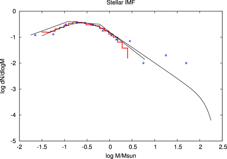
Figure 1.— The analytical stellar IMF that we use for our MC experiments compared with the IMF of the Trapezium cluster by Hillenbrand and Carpenter [2000], steps; Luhman et al. [2000], segmented solid lines; and Muench et al. [2002], asterisks.

We sample the Salpeter IMF to create clusters with n stars assuming a scale-free frequency distribution $P(n)\propto n^{\beta}$, and we build the cluster mass spectrum using Equation 10,

$$\xi_{cl}(M)=\sum_{n=1}^{\infty}F_{n}(M)P(n),$$

where $F_{n}(M)$ is the mass distribution function of clusters with exactly $n$ stars. Notice that this process is scale-free only if the sum starts from $n=1$, in which case the only mass scales of the problem are $m_{l}$ and $m_{u}$, the lower and upper mass cut-offs of the stellar IMF. Our Monte Carlo simulations consist of repeatedly drawing n stars from the Salpeter IMF, calculating $M=m_{1}+\cdots+m_{n}$ as the mass of a cluster with n stars, and then obtaining $F_{n}(M)$.

For the value of $\beta$ there have been a multitude of studies of massive clusters in galaxies, which gives for the mass functions values ranging between $\beta=-1.85$ [de Grijs and Anders, 2006] to $\beta=-2.4$ [Hunter et al., 2003]. More extensive references are given in Elmegreen [2006]. For smaller clusters de Wit et al. [2004, 2005] claim that their data on isolated massive star formation can be understood if $\beta=-1.7$. For massive clusters one can directly use the same exponent for the mass function as for $P(n)$ because, as discussed above, the total mass scales with $n$ and the width for fixed $n$ scales with $\sqrt{n}$. In this work we will explore $\beta=-1.8,-2.0$, and $-2.2$.

3. Comparison with observations

We have identified two observational tests that can be performed to check the validity of our null hypothesis. First, we will see if we can reproduce the form of the embedded cluster mass function; second, we will see if we can reproduce the statistics of the most massive star in clusters. We are aware that we are leaving out tests regarding the characteristics of small $n$  multiple systems, which could falsify it. But multiple systems, although numerous, are not the main source of stars in the field, so they will not affect the main conclusions of the present work, namely that the stellar and cluster field IMF can be the same.

3.1. The embedded cluster mass function

Due to the difficulty defining unbiased complete samples, the important range of clusters masses in the regime of stellar masses is not well studied. There are nevertheless two relatively recent sources based on extensive surveys of the literature at the time of publication: Porras et al. [2003] and Lada and Lada [2003]. We prefer to use LL2003 four our analysis because they give estimates of the masses of the clusters, although only 4 of the clusters in the Porras et al. list that satisfy the constraint on minimum number of stars of LL2003 are not included in this catalog. The cluster masses given in LL2003 were obtained by modeling source counts as a function of limiting magnitudes for two model clusters with ages of 0.8 Myr and 2 Myr, corresponding to the ages of the Trapezium and IC 348 clusters respectively. They assumed a universal IMF and used the average of the mass determined for the two assumed ages.

Figure 2 shows the empirical data of LL2003 together with the results of six runs of our MC experiments in which we built clusters with the above $P(n)$ for $n\geq 35$, drawing 72 clusters at the time (the parameters of the observations of LL2003). We note the excellent agreement between the simulations and LL2003 except for the mass bins at $\log M\sim 0.95$ and $\log M\sim 3.5$ which are totally de-populated in LL2003. For $\beta=-1.8$ the smallest mass bin is de-populated in 15% of our simulations while in 70% of the simulations contains 2 clusters or less. The highest mass bin is populated in only $\sim 40\%$ of the simulations and in almost 100% of the simulations contains less than 2 clusters. LL2003 proposed that the downturn at smaller masses was evidence for a favored cluster formation mass scale at around $M\sim 50M_{\odot}$. However, our simulations indicate that this downturn is naturally explained by the cutoff in n they introduced in an otherwise scale-free spectrum, without the need to invoke a special cluster formation scale. The figure shows that the data is best modeled if the cutoff in $n$ is a bit larger than the LL2003 criterion of $n>35$ to select clusters. This is probably the effect of having a sample with an inhomogeneous magnitude limit so that $n>35$ becomes only a lower limit to the actual cutoff.

Figure 2.— The Lada and Lada (2003) spectrum of masses of embedded clusters together with the results of Monte Carlo simulations in which we sample the stellar IMF with a number probability distribution $\beta={-1.8}$, top row; $\beta={-2.0}$, middle row; $\beta={-2.2}$, bottom row. For $n\geq 35$, left column; and $n\geq 70$, right column.

3.2. The statistics of the maximal mass star in clusters

WK2006 argued that their observed correlation between the maximal star mass and the total mass of clusters is not consistent with the hypothesis that clusters are formed by random sampling of a universal stellar IMF. WK2006’s sample of clusters is strongly affected by a size-of-sample effect (see Appendix A). Because of the impracticality of finding a large ensemble of small clusters and thus avoid the problems introduced by the size-of-sample effect, WK2006 performed Monte Carlo experiments to determine the statistical properties of each of their three sampling methods. We were puzzled by their Figure 3, which shows that for their random sampling method (that corresponds to our Monte Carlo models), the curves of maximal mass star versus cluster mass ($M_{ecl}$) have two maxima in the range between $\sim 25M_{\odot}$ and $\sim 250M_{\odot}$. For example, for $M_{ecl}=100M_{\odot}$ the curve peaks at $\sim 10~{}M_{\odot}$ and then again at $\sim 100~{}M_{\odot}$. Since it is precisely in this mass range that the model curve departs most strongly from the data points, we thought that the double peaks could be the result of a computational error. We therefore decided to repeat the calculations using our independent algorithm to build the bivariate (maximal stellar mass – cluster mass) probability distribution. The results of our simulations are shown Figure 3, where, much to our surprise, we reproduce the double peaks obtained by WK2006!

Figure 3 shows the results of many MC experiments of the random sdampling model from which we have calculated the bivariate probability distribution to have a cluster in a given log-mass bin of width 0.5, with a star of maximal mass in a log-mass bin of width 0.1. Lighter areas correspond to a higher probability. Figure 3a correspond to MC experiments in which anything is considered a cluster, even system with n=1. Figure 3b considers only cluters with n$>$50. The vertical line in Figure 3a marks the position of $\log M=1.8$. Notice that as one moves from bottom to top along this line one will cross contour levels that at first increase until the bivariate distribution reaches a maximum at $\log m^{*}_{max}\approx 0.9$. If one continues to move it will reach a minimum at approximately $\log m^{*}_{max}\approx 1.4$, and then it starts increasing again reaching a maximum at the point in which all the cluster mass is in a single star. Notice that this double (local) maxima feature comes from the nature of the probability distribution of star masses conditioned to cluster mass ((Fig 4, see below).

Interestingly, the clusters from the compilation of Weidner and Kroupa [2006] (crosses in Fig. 3) all concentrate in the ridge of the distribution defined by the first (lower mass) peak described above and do not cover the full mass range allowed by our models. To a lesser extent this is also true of the models by Weidner and Kroupa [2006], whose Figures 4 and 5 show the data to have a much smaller dispersion around the mean than the models. Nevertheless, the random sampling method deviate most from the data due to its “double peaked” mass distribution. With our preferred random sampling method clusters with masses in the stellar mass range the most massive stars can have masses similar to the total cluster mass. Moreover, the conditional probability distribution of stellar masses, $P(m|M)$, for clusters in the stellar mass range shows that some clusters can be dominated by one or at most a few high mass stars (Fig 4). This increase in the probability distribution of stellar masses near the cluster mass is also visible in Figure 2 of Durisen et al. [2001], so the critical questions are whether this effect is real, and if so, whether it is significant. The fact that the effect is seen in three independent investigations argues strongly for the reality of the peak in the random sampling model, but its significance is debatable. On the one hand, the effect arises from partitioning the data into mass bins, and it is forced into existence by the need to satisfy Equation 14, so it is of no physical significance. On the other hand, it biases (toward large values) the mean maximal stellar mass versus cluster mass curve used by Weidner and Kroupa [2006] to falsify the random sampling model, so it is highly significant.

Is this a real violation of our null hypothesis signaling the presence of some interesting physical effect or is it the effect of improper data, or its analysis, or both? Although WK2006’s conclusions are based on a very limited data-set, it is unlikely that this alone can explain the difference in the distribution of the data points and that predicted by the models: the number of clusters in each mass bin is small but the total sample is not that small and at all masses the data points are delineating the lowest maximal stellar mass ridge of the distribution.

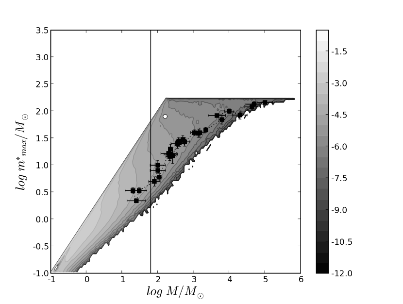
Figure 3.— (a, top) The bivariate probability distribution function of maximum stellar mass and cluster mass. The overlaid points correspond to the data in Weidner and Kroupa [2006]. This figure show the result with a cluster $P(n)\sim 1/n^{2}$ starting at n=1. The grey levels correspond to the bivariate probability of finding a cluster in a log-mass bin of size $0.5\times 0.1$. The white circle represents WR20a taken as a system. The points represent the data points in WK2006 with a few additions from Weidner (2007). The vertical line is drawn at a log M value of 1.8. (b, bottom) Same as (a) but with $n>50$. For details see main text.

Figure 4.— Conditional probability distributions of stellar masses conditioned to cluster mass. The topmost curve correspond to P(m) where the cluster mass has bin marginalized. The other curves correspond from top to bottome to P(m—M) for log M equal to -1.25, -0.75, -0.25, 0.25, 0.75, 1.25, 1.75, 2.25, 2.75, 3.25, 3.75, and 4.25 respectively.

One possible explanation could come from the highly hierarchical nature of young stellar systems and the somewhat arbitrary way in which the parent object of the maximal star is chosen. For example, the cluster Westerlund 2 has the well known massive binary WR20a, both components of which with masses $\sim 80M_{\odot}$ [Rauw et al., 2004, 2005]. Considering that the ratio of its components separation to the cluster size is smaller than the ratio of the cluster size to that of the Milky Way, there is no objective reason not to have such binary star as a single point in Figure 3, in which case we would have a data point in the area devoid of points in that Figure. An objective algorithm to identify clusters of different number of stars is needed. A step in that direction is the work of Oey et al. [2004] which used the algorithm by Battinelli [1991] to identify groupings of stars and showed that the distribution of clusters by number of stars is consistent with $n^{-2}$ down to single stars. What is needed is then to determine the maximal mass star and total mass of those clusters to build the bivariate probability distribution.

Finally, another explanation is that these data do indeed falsify our null hypothesis and that they signal the presence of some interesting physical effect that results in the mass of the most massive star to depend on the mass of its parent cluster. One possibility could be that stars form in an ordered fashion, less massive stars forming first. Once a high mass star is formed this one cleans the cluster of its placental material and the cluster rapidly disintegrate [Elmegreen, 1983]. This is the explanation favoured by WK2006. But there is another possibility: clusters with maximal mass star of too large masses can be more gravitationally unstable. A cluster with a maximal mass star of very large mass is characterized also by having a smaller total number of stars, and its conditional stellar mass function is flatter (see Figure 4). Terlevich [1987] found that a flatter mass spectrum results in a considerably smaller half-life: her model XV evolves an order of magnitude faster that a cluster with a normal Salpeter IMF. This explanation has the feature that it does not violate the null hypothesis, because clusters are formed according to the random sampling model but their lifetimes, and thus the probability of observing them, depend on the mass of the maximal stellar mass in them.

4. Discussion

As mentioned in the Introduction, our results depart radically from those of KW2003. Their conclusion that the field built by clusters must have a steeper stellar IMF can be criticized on several accounts as follows. To begin, as noted by Elmegreen [2006], for the observed range of cluster masses, the predicted steepening in the stellar IMF is rather small going from $\Gamma=-1.35$ in clusters to $\Gamma\sim-1.5$ in the field (Figure 2 in KW2003). This is well within the observed variance in the stellar IMF of clusters, and can be comfortably ascribed to systematic errors in the determination of the slope [see e.g. Kroupa, 2002].

A second problem is that KW2003 implicitly assume that the cluster mass spectrum is well determined down to masses comparable to those of the smaller stars and is approximately given by $\xi_{cl}\sim M^{-2}$ for $5\leq M/M_{\odot}\leq 10^{7}$. As mentioned in the previous section, however, LL2003 claim that the cluster mass spectrum turns abruptly down for masses below $M\sim 50M_{\odot}$, that is, it appears to have a preferred mass-scale. This reduces the number of small mass clusters thus reducing the predicted difference between cluster stellar IMF and the field. Almost paradoxically, our model invoking a universal stellar IMF shows that this preferred mass-scale is most likely not a physically significant feature of cluster formation!

Another problem is that KW2003 use a Procrustean approach in their modeling of clusters where all clusters are forced to have one maximal mass star, that is, a star of the maximum mass allowed by the stellar IMF. This assumption,

$$1=\int_{m_{max*}}^{m_{u}}f(m)dm,$$ (16)

forces the upper mass cut-off of the IMF to be an increasing function of cluster mass, varying as $M^{1/x}$. From the discussion leading to Equation 14 it is clear that we can not recover the input IMF unless we include in our sums clusters for which $m=M$.

Elmegreen [2006] expanded the formalism of Vanbeveren and showed analytically and numerically that for a power-law mass distribution of clusters of slope $\beta\leq 2$, the summed IMF of a population of clusters is indistinguishable from the cluster IMF. However, the functional form of the conditional probability $P(m|M)$ adopted by Elmegreen does not satisfy Equation 14 for any value of $\beta$; it just happens that for $\beta\leq 2$ the summed IMF is almost the same as the cluster IMF (they differ by a logarithmic multiplicative factor). This clearly shows that the finding of KW2003, that for $\beta>2$ the summed IMF becomes significantly steeper than the individual cluster IMF, arises from the assumption that, besides a normalization factor that depends on the cluster mass through Equation 16, $P(m)$ and $P(m|M)$ have the same functional form, (simple power-laws of the same slope in the case of Elmegreen). While this is a very good assumption for very massive clusters, it clearly does not apply for clusters in the stellar mass range which are the ones responsible for “tilting” the sum-IMF for $\beta>2$. Thus, even within the Vanbeveren formalism the IMF of clusters and the field can be strictly the same for any cluster mass distribution.

The results of WK2006 are confirmed in this work in the sense that we also find that real clusters cover a significantly smaller part of the maximal stellar mass and cluster mass space than permitted by the random sampling model. WK2006 go then to modify their sampling algorithm in such a way as to reduce the probability of having very large mass stars in their clusters arguing that “Star clusters appears to form in an ordered fashion, starting with the lowest-mass stars until feedback is able to outweigh the gravitationally induced formation process.” Although this is a possible scenario we favour a different one in which the area of the bivariate distribution allowed by the random sampling model is rendered unstable due to the extreme nature of the mass spectrum therein, in accordance with the simulations of Terlevich [1987]. How much “trimming” of the bivariate distribution can be actually accomplished this way will be the subject of a future work.

Our strong conclusion is that the observations of the stellar IMF and the mass spectrum of young clusters are consistent with the hypothesis that clusters form by random sampling of a universal stellar IMF. This conclusion leads us to challenge the received hypothesis that clusters are the fundamental building blocks of the stellar populations in galaxies [de Wit et al., 2004, 2005]. In this view clusters are given an independent existence from before the time that stars form. In our view, following the ideas of Elmegreen (1997), stars form in giant molecular clouds in a hierarchy of structures with different numbers and masses. Some of these structures end up forming large clusters (which will later dissolve) and some don’t: they become part of small associations of stars formed in neighboring regions almost by chance. In fact, the observations of de Wit et al. (2004, 2005), that are used as standard references for the view that clusters form first, find that 30% of young massive Galactic field stars are not members of clusters or OB associations. Of these, about 50% are runaway star candidates. They conclude that 4$\pm 2\%$ of the stars in their sample result from truly isolated high-mass star formation, a number that can be reproduced “assuming that all stars are formed in clusters that follow a universal cluster distribution (by $N_{*}$) with slope $\beta\sim-1.7$ down to clusters with a single member.” If we consider single star clusters the statement that all stars are formed in clusters becomes a tautology.

Our results hint at a strong universality hypothesis for the IMF where not only the power-law part, but the full function may be universal. Clearly this claim has profound implications for understanding how stars form and therefore its foundations require considerably more observational work than was available for the tests presented in this paper.

5. Summary

This paper combines four separate results within a single unified view. The unification is actually a result of Equation 11 (that is derived formally in the first section of the paper) which relates the cluster mass function with the probability distribution of number of stars in clusters, and the (universal) stellar IMF. These results are

• the IMF of a field stellar population and that of the clusters out of which the field was built can be strictly the same. This result contradicts Kroupa and Weidner [2003], and was implicit in the models by Larson [1982], Oey and Clarke [2005a, b], and de Wit et al. [2004];

• the observations of the lower end of the cluster mass function, as given by Lada and Lada [2003], agree with the random sampling model presented here if: (a) the distribution of clusters by the number of stars they contain is a scale-free power law, $n^{\beta}$, with $\beta$ between -1.8 and -2.2; (b) the stellar IMF is independent of $n$ and it is given by the Salpeter form;

• the observed special mass scale for cluster formation claimed by Lada and Lada arises from the arbitrary cut-off in the number of stars imposed by them;

• the interpretation of the statistics of the most massive star in clusters is a valuable tool to study cluster formation processes as the observations, taken at face value, violate the null hypothesis represented by the random sampling model. Although a proper observational study requires a sample including many clusters with only a few members, we believe that the observations presented by WK2006 are at worst compelling. Nevertheless, it is argued in the present work that the discrepancy is due to systems which are rendered gravitationally unstable by the presence of one or more very massive stars.

Appendix A Size-of-sample effect

The size-of-sample effect arises in many areas of astronomy, and we have studied it in the context of the distribution of sizes of super-associations in galaxies  (Selman and Melnick, 2000). The formalism developed there can be translated mutatis mutandi to the present context as follows: Let the whole set of star clusters to be analyzed be denoted by ${\cal C}=\{C_{i}\}_{i=1}^{N}$, where $C_{i}$ is the i-th cluster with mass $M_{i}$ and maximum stellar mass $m^{max*}_{i}$. We will assume ${\cal C}$ to be ordered from the most massive to the least massive cluster, that is, $i<j\Rightarrow M_{i}>M_{j}$. Let $M_{l}=\sum_{i=1}^{l}M_{i}/l$ be the average mass of the $l$ most massive clusters. From ${\cal C}$ we will draw $N_{S}$ sub–samples, ${\cal S}_{j}$, of equal mass, $M_{l}$, defined by

$${\cal S}_{j}=\{C_{i}\}_{i=j}^{n_{j}},$$

where $n_{j}$ is defined by the expression,

$$\sum_{i=j}^{n_{j}}M_{i}=M_{l}.$$

Thus, the sub-sample ${\cal S}_{j}$ contains the cluster $C_{j}$ and the next $n_{j}-1$ less massive clusters, enough to add up to a total mass equal to $M_{l}$. We will assign to each sub-sample $j$ two numbers: $\tilde{m}^{max*}_{j}$, and $\tilde{M}^{avg}_{j}$, defined as

$$\tilde{m}^{max*}_{j}=\max_{C_{i}\in{\cal S}_{j}}m^{max*}_{i},$$

$$\tilde{M}^{avg}_{j}={1\over{n_{j}-j+1}}\sum_{i=j}^{n_{j}}M_{i}.$$

$\tilde{m}^{max*}_{j}$ is equal to the maximum stellar mass of all the members of ${\cal S}_{j}$, and $\tilde{M}^{avg}_{j}$ their average mass. We will refer to sub–sample j as “super–cluster” j. Because all “super–clusters” thus defined have approximately equal total mass ($\approx M_{l}$), we can compare the mass of their maximal star without having a size–of–sample effect.

Figure 5.— The maximum stellar mass in a sub-sample of the data of WK2006 analyzed as detailed in the main text. The x-axis show the average mass of the clusters in the 800 M_⊙ “super clusters”, while the y-axis show the mass of the maximal mass star in the super clusters.

Regrettably, the data set and the metod of analysis used by WK2006 is far from what is needed for this kind of analysis. Their Table 1 lists 17 clusters with masses ranging from $25M_{\odot}$ to $10^{5}M_{\odot}$. We have seen that we should actualy work with the number of stars instead of the mass of the clusters as conditioning to cluster mass introduces unphysical mass scales. If we use an average stellar mass of $0.3M_{\odot}$ then the smallest mass cluster corresponds to a cluster with $\approx$ 75 stars while the largest mass clusters corresponds to $\approx 3\times 10^{5}$ stars. The sample should include at least 4000 clusters with 75 stars to meaningfully compare the maximal mass of this artificial “super-cluster” with the maximal mass of a cluster of $10^{5}M_{\odot}$ (such as R136). Figure 5 plots the maximal mass against total mass for the best sub-sample of “super-clusters” that can be constructed from the data of WK2006 using the algorithm described above. This sample consists of NGC6530 as the first “super-cluster”; NGC 2264, Mon R2, and $\sigma$ Ori in the second; Mon R2, $\sigma$ Ori, NGC 2024, and IC 348 in the third; and $\sigma$ Ori, NGC 2024, IC 348, $\rho$ Oph, NGC 1333, Ser SVS2, and Taurus-Auriga in the fourth. Each of these four “super-clusters” has a total mass of approximately 800 M_⊙. The “best-set” shows no correlation between maximal star mass and cluster richness: the claimed correlation was a size-of-sample effect. (It is possible to construct other sub-samples having a more massive star in the upper mass bin, but these sub-samples contain only 2 or 3 super-clusters.)

References

- Battinelli [1991] P. Battinelli. A&A, 244:69, 1991.
- Brandt [1998] S. Brandt. Data Analysis. Springer-Verlag, New York, 1998.
- Cerviño et al. [2002] M. Cerviño, D. Valls-Gabaud, V. Luridiana, and J. M. Mas-Hesse. A&A, 381:51, 2002.
- de Grijs and Anders [2006] R. de Grijs and P. Anders. MNRAS, 366:295, 2006.
- de Wit et al. [2004] W. J. de Wit, L. Testi, F. Palla, L. Vanzi, and H. Zinnecker. A&A, 425:937, 2004.
- de Wit et al. [2005] W. J. de Wit, L. Testi, F. Palla, and H. Zinnecker. A&A, 437:247, 2005.
- Durisen et al. [2001] R. H. Durisen, M. F. Sterzik, and B. K. Pickett. 952:952, 2001.
- Elmegreen [1983] B. G. Elmegreen. MNRAS, 203:1011, 1983.
- Elmegreen [2006] B. G. Elmegreen. ApJ, 648:572, 2006.
- Gouliermis et al. [2005] D. Gouliermis, W. Brandner, and Th. Henning. ApJ, 623:846, 2005.
- Hillenbrand and Carpenter [2000] L. A. Hillenbrand and J. M. Carpenter. ApJ, 540:236, 2000.
- Hunter et al. [2003] D. A Hunter, B. G. Elmegreen, T. J. Dupuy, and M. Mortonson. AJ, 126:1836, 2003.
- Kendall and Stuart [1977] M. Kendall and A. Stuart. The advanced theory of statistics. Charles Griffin and Company, London, 1977.
- Kroupa [2002] P. Kroupa. Science, 295:82, 2002.
- Kroupa and Weidner [2003] P. Kroupa and C. Weidner. ApJ, 598:1076, 2003.
- Lada and Lada [2003] C. J. Lada and E. A. Lada. ARA&A, 41:57, 2003.
- Larson [1982] R. B. Larson. MNRAS, 200:159, 1982.
- Luhman et al. [2000] K. L. Luhman, G. H. Rieke, E. T. Young, A. S. Cotera, H. Chen, M. J. Rieke, G. Schneider, and R. I. Thompson. ApJ, 540:1016, 2000.
- Massey [2002] P. Massey. ApJS, 141:81, 2002.
- Massey et al. [1995] P. Massey, C. C. Lang, K. DeGioia-Eastwood, and C. Garmany. ApJ, 438:188, 1995.
- McDonald and Clarke [1993] J. M. McDonald and C. J. Clarke. MNRAS, 262:800, 1993.
- Morse and Feshbach [1953] P. M. Morse and H. Feshbach. Methods of theoretical physics. McGraw-Hill, New York, 1953.
- Muench et al. [2002] A. A. Muench, E. A. Lada, C. J. Lada, and J. Alves. ApJ, 573:366, 2002.
- Oey and Clarke [2005a] M. S. Oey and C. J. Clarke. AJ, 115:1543, 2005a.
- Oey and Clarke [2005b] M. S. Oey and C. J. Clarke. ApJ, 620:43, 2005b.
- Oey et al. [2004] M. S. Oey, N. L. King, and J. Wm. Parker. AJ, 127:1632, 2004.
- Porras et al. [2003] A. Porras, C. Micol, J. Di Francesco, T. S. Megeath, and P. C Myers. AJ, 126:1916, 2003.
- Rauw et al. [2004] G. Rauw, M. De Becker, Y. Nazé, P. A. Crowther, E. Gosset, H. Sana, K. A. van der Hucht, J.-M. Vreux, , and P. M. Williams. A&A, 420L:9, 2004.
- Rauw et al. [2005] G. Rauw, P. A. Crowther, M. De Becker, E. Gosset, Y. Nazé, H. Sana, K. A. van der Hucht, J.-M. Vreux, and P. M. Williams. A&A, 432:985, 2005.
- Reddish [1978] V. C. Reddish. Star formation. Pergamon Press, 1978.
- Salpeter [1955] E. E. Salpeter. ApJ, 121:161, 1955.
- Scalo [1986] J. Scalo. Fund. Cosmic Phys., 11:1, 1986.
- Selman and Melnick [2005] F. Selman and J.. Melnick. A&A, 443:851, 2005.
- Sterzik and Durisen [1998] M. F. Sterzik and R. H. Durisen. A&A, 339:95, 1998.
- Terlevich [1987] E. Terlevich. MNRAS, 224:193, 1987.
- van Albada [1968a] T. S. van Albada. Bull. Astr. Inst. Netherlands, 19:479, 1968a.
- van Albada [1968b] T. S. van Albada. Bull. Astr. Inst. Netherlands, 20:57, 1968b.
- Vanbeveren [1982] D. Vanbeveren. A&A, 115:65, 1982.
- Weidner and Kroupa [2006] C. Weidner and P. Kroupa. MNRAS, 365:1333, 2006.
- Zinnecker and Yorke [2007] H. Zinnecker and H. W. Yorke. ARA&A, 45:481, 2007.