Abundances of lithium, sodium, and potassium in Vega

Abstract

Vega’s photospheric abundances of Li, Na, and K were determined by using considerably weak lines measured on the very high-S/N spectrum, while the non-LTE correction and the gravity-darkening correction were adequately taken into account. It was confirmed that these alkali elements are mildly underabundant ([Li/H] $\simeq-0.6$, [Na/H] $\simeq-0.3$, and [K/H] $\simeq-0.2$) compared to the solar system values, as generally seen also in other metals. Since the tendency of Li being more deficient than Na and K is qualitatively similar to what is seen in typical interstellar cloud, the process of interstellar gas accretion may be related with the abundance anomaly of Vega, as suspected in the case of $\lambda$ Boo stars.

1 Introduction

While Vega (= $\alpha$ Lyr = HR 7001 = HD 172167 = HIP 91262; A0V) plays an important role as the fundamental photometric standard, its photospheric chemical composition is known to be sort of anomalous. Namely, most elements are mildly underabundant (by $\sim-0.5$ dex on the average) in spite of its definite population I nature, though the extent of deficiency is inconspicuous for several volatile elements of low condensation temperature ($T_{\rm c}$) such as C, N, O, and S. Since this is the tendency more manifestly shown by a group of A–F main-sequence stars known as “$\lambda$ Boo-type stars” (see, e.g., Paunzen 2004 and the references therein), Vega’s moderate abundance peculiarities have occasionally been argued in connection with this $\lambda$ Boo phenomenon (e.g., Baschek & Slettebak 1998; Stürenburg 1993; Holweger & Rentzsch-Holm 1995; Ilijić et al. 1998).

Regarding the origin of unusual surface compositions of $\lambda$ Boo stars, various models have been propounded so far, such as the diffusion/mass-loss model, accretion/diffusion model, or binary model (see the references quoted in Paunzen 2004). Among these, the interpretation that the anomaly was built-up by the accretion of interstellar gas (where refractory metals of high $T_{\rm c}$ are depleted because of being condensed into dust while volatile species of low $T_{\rm c}$ hardly suffer this process), such as the interaction model between a star and the diffuse interstellar cloud proposed by Kamp & Paunzen (2002), appears to be particularly promising, in view of Paunzen et al.’s (2002) recent finding that the [Na/H] values of $\lambda$ Boo stars (showing a large diversity) are closely correlated with the [Na/H]_ISM values (sodium abundance of interstellar matter) in the surrounding environment (cf. Fig. 7 therein).

Then, according to the suspected connection between Vega and $\lambda$ Boo stars, it is natural to examine the photospheric Na abundance of Vega. Besides, the abundances of Li and K may also be worth particular attention in a similar analogy, since these three alkali elements play significant roles in discussing the physical state of the cool interstellar gas through their interstellar absorption (resonance) lines of Na i 5889/5896 (D₁/D₂), Li i 6708, and K i 7665/7699.

It is somewhat surprising, however, that reliable determinations of Vega’s Na abundance are barely available. To our knowledge, although a number of abundance analyses of Vega have been published so far over the past half century, Na abundance derivations were done only in four studies (among which original $W_{\lambda}$ measurements were tried only two of these) according to our literature survey: Hunger (1955; Na i 5889/5896), the reanalysis of Hunger’s $W_{\lambda}$ data by Strom, Gingerich & Strom (1966), Qiu et al. (2001; Na i 5896), and the reanalysis of Qiu et al’s $W_{\lambda}$ data by Saffe & Levato (2004). Unfortunately, none of these appear to be sufficiently credible as viewed from the present knowledge, because of neglecting the non-LTE effect for the strong resonance D₁/D₂ lines which were invoked in all these studies (see below in this section).

The situation is even worse for Li and K, for which any determination of their abundances in Vega has never been reported. Gerbaldi, Fraggiana & Castelli (1995) once tried to measure the $W_{\lambda}$(Li i 6708) value of Vega and derived a tentative value of 2 m$\rm\AA$, which was not used however, since they did not regard it as real under the estimated ambiguity of 4 m$\rm\AA$ (cf. their Table 6). Regarding the K i 7665/7699 lines, even a trial of measuring their strengths has never been undertaken for Vega, as far as we know.

Several reasons may be enumerated concerning this evident scarcity of investigations on Li, Na, and K (which actually holds for early-type stars in general):
— First of all, since the strengths of Li i, Na i, and K i lines quickly fade out as $T_{\rm eff}$ becomes higher owing to the enhanced ionization of these alkali atoms (only one valence electron being weakly bound), one has to contend with the difficult task of measuring very weak lines (e.g., $W_{\lambda}$ value even as small as $\sim$ 1m$\rm\AA$), which requires a spectrum of considerably high quality.
— Second, these lines situate in the longer wavelength region of yellow–red to near-IR, where many telluric lines due to H₂O or O₂ generally exist to cause severe blending with stellar lines, which often prevent us from reliable measurements of equivalent widths. (see, e.g., Sect. 6.2 of Qiu et al. 2001, who remarked the large uncertainty caused by this effect in their measurements of Na i D lines).
— Third, the resonance lines in the longer wavelength region are generally known to subject to considerable non-LTE corrections especially for the case of Na i 5889/5896 lines showing considerable strengths. Unfortunately, since detailed non-LTE studies of these alkali elements have been rarely published as far as early-type (A–F) dwarfs are concerned, lack of sufficient knowledge on non-LTE corrections may have hampered investigating their abundances.

Given this situation, we decided to spectroscopically establish Vega’s photospheric abundances of Li, Na, and K scarcely investigated so far, while overcoming the problems mentioned above, in order to see how they are compared with the compositions of other elements in Vega as well as with those of interstellar gas. This is the purpose of this study.

This attempt was originally motivated by our recent work (Takeda, Kawanomoto & Ohishi 2007) of publishing a digital atlas of Vega’s high-resolution ($R\sim 100000$) and high-S/N ($\sim$ 1000–3000) spectrum along with that of Regulus (a rapid rotator to be used for a reference of contaminating telluric lines), by which the confronted main obstacles (the necessity of measuring very weak lines as well as removing telluric blends) may be adequately conquered. Besides, regarding the technical side of abundance determinations, we are ready to evaluate not only the necessary non-LTE corrections for Li, Na, and K (according to our recent experiences of statistical equilibrium calculations on these elements for F–G–K stars), but also the gravity-darkening corrections which may be appreciable especially for very weak lines as revealed from our recent modeling of rapidly-rotating Vega (Takeda, Kawanomoto & Ohishi 2008). Therefore, this would make a timely subject to address.

2 Observational data

The basic observational data of Vega used for this study are the high-S/N ($\sim$ 1000–3000) and high resolution ($R\sim 100000$) spectra, which are based on the data obtained with the HIgh Dispersion Echelle Spectrograph (HIDES) at the coudé focus of the 188 cm reflector of Okayama Astrophysical Observatory. These spectral data of Vega, along with those of Regulus (a rapid rotator serving as a reference of telluric lines) were already published as a digital atlas by Takeda et al. (2007) which may be consulted for more details.

The following 11 lines were selected as the target lines used for abundance determinations: Na i 5890/5896, 8183/8195, 6154/6161, 5683/5688, K i 7665/7699, and Li i 6708 (cf. Table 1). Since most of these wavelength regions (except for those of Na i 6154/6161 and Li i 6708) are contaminated by telluric lines, these features were removed by dividing Vega’s spectra by the reference spectra of Regulus (with the help of IRAF task telluric) which are also included in Takeda et al. (2007) along with the airmass information. Though this removal process did not always work very successfully (e.g., for the case of very strong saturated lines such as the O₂ in the K i 7665/7699 region and the H₂O lines in the Na i 8183/8195 region), we could manage to recover the intrinsic stellar lines more or less satisfactorily, since none of these target lines fortunately coincided with the deep core positions of such very strong telluric features.

While most of the lines were confidently identified by comparing them with the theoretically simulated spectra, the detection of the extremely weak Li i 6708 line was still uncertain in the original spectrum even at its very high S/N ratio of $\sim 2000$. Therefore, an extra smoothing was applied to the spectrum portion in the neighborhood of this line by taking a running mean over 9 pixels, by which the feature became more distinct (cf. Fig. 6) thanks to the further improved S/N ratio by a factor of 3.

The measurements of the equivalent widths (with respect to the local continuum level specified by eye-inspection) were done by the Gaussian-fitting technique, and the resulting $W_{\lambda}$ values are given in Table 1. The relevant spectra at each of the wavelength regions are shown in Figs. 1 (Na i 5890/5896), 2 (Na i 8183/8195), 3 (Na i 6154/6161), 4 (Na i 5683/5688), 5 (K i 7665/7699), and 6 (Li i 6708).

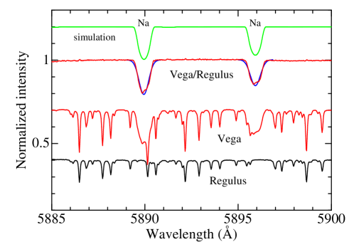
Figure 1: Spectra of 5885–5900 $\rm\AA$ region comprising Na i 5890 and 5896 lines. Theoretical simulation (LTE, broadened with $v_{\rm e}\sin i=22$ km s^-1), Vega/Regulus (telluric lines removed), raw Vega, and raw Regulus are arranged from top to bottom with appropriately chosen offsets. The scale of the ordinate corresponds to the second-top spectrum, for which equivalent-widths of these lines were measured by the Gaussian fitting method (as overplotted in solid lines on this spectrum).

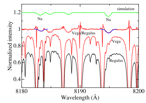
Figure 2: Spectra of 8180–8200 $\rm\AA$ region comprising Na i 8183 and 8195 lines. Theoretical simulation, Vega/Regulus (telluric lines removed), raw Vega, and raw Regulus are arranged from top to bottom with appropriately chosen offsets. Otherwise, the same as in Fig. 1.

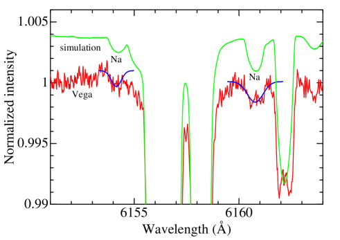
Figure 3: Spectra of 6151–6164 $\rm\AA$ region comprising Na i 6154 and 6161 lines. Theoretical simulation (upper) and raw Vega (lower) are placed with an appropriate offset. This region is not contaminated by telluric lines. Otherwise, the same as in Fig. 1.

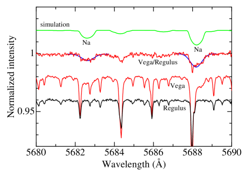
Figure 4: Spectra of 5680–5690 $\rm\AA$ region comprising Na i 5683 and 5688 lines. Theoretical simulation, Vega/Regulus (telluric lines removed), raw Vega, and raw Regulus are arranged from top to bottom with appropriately chosen offsets. Otherwise, the same as in Fig. 1.

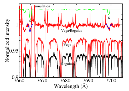
Figure 5: Spectra of 7660–7705 $\rm\AA$ region comprising K i 7665 and 7699 lines. Theoretical simulation, Vega/Regulus (telluric lines removed), raw Vega, and raw Regulus are arranged from top to bottom with appropriately chosen offsets. Otherwise, the same as in Fig. 1.

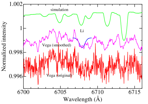
Figure 6: Spectra of 6700–6716 $\rm\AA$ region comprising Li i 6708 merged doublet. Theoretical simulation, smoothed Vega spectrum by convolving the 9-pixel boxcar function, and raw Vega spectrum are arranged from top to bottom with appropriately chosen offsets. This region is hardly contaminated by telluric lines. Otherwise, the same as in Fig. 1.

3 Abundance determinations

Regarding the fiducial atmospheric model of Vega, Kurucz’s (1993) ATLAS9 model with the parameters of $T_{\rm eff}=9550$ K (effective temperature), $\log g$ (cm s^-2) = 3.95 (surface gravity), [X/H] = $-0.5$ (metallicity), and $v_{\rm t}$ = 2 km s^-1 (microturbulence) was adopted for this study as in Takeda et al. (2007), which appears to be the best as far as within the framework of classical plane-parallel ATLAS9 models according to Castelli & Kurucz (1994).

As the basic strategy, the LTE abundance ($A_{\rm LTE}$) was first derived from the measured $W_{\lambda}$ by using the WIDTH9 program,, to which the non-LTE correction ($\Delta_{\rm NLTE}$) and the gravity-darkening correction ($\Delta_{\rm GD}$) were then applied to obtain the final abundance ($A_{\rm NLTE+GD}$).

In this step-by-step way, one can quantitatively judge the importance/unimportance of each effect by comparing two abundance corrections, and such factorized information may be useful in application to other different situations (e.g., the case of slow rotator where only $\Delta_{\rm LTE}$ is relevant; cf. Appendix A). Also, the use of “relative correction” (instead of directly approaching the absolute abundance solution) has a practical merit of circumventing the numerical-precision problem involved in the spectrum computation on the gravity-darkened model (especially seen for the case of the extremely weak Li i 6708 line composed of several components; cf. footnote 9).

The non-LTE calculations for evaluating $\Delta_{\rm NLTE}$ were carried out in the same manner as described in Takeda et al. (2003; Na i), Takeda & Kawanomoto (2005; Li i), and Takeda et al. (2002; K i). Besides, all the relevant atomic data ($gf$ values, damping constants, etc.) for abundance determinations were so adopted as to be consistent with these three studies.

The gravity-darkening corrections ($\Delta_{\rm GD}$) were derived based on the equivalent-width intensification factor computed by the program CALSPEC under the assumption of LTE ($W_{4}/W_{0}$, where $W_{4}$ and $W_{0}$ correspond to the gravity-darkened rapid rotator model and the classical rigid-rotation model, respectively; and the abundance was adjusted to make $W_{4}$ consistent with $W_{\lambda}^{\rm obs}$), the details about which are explained in Takeda et al. (2008). Practically, the relation $\Delta_{\rm GD}=-\log(W_{4}/W_{0})$ was assumed for the very weak lines ($W_{\lambda}<15$ m$\rm\AA$; i.e., Na i 6154/6161, Na i 5683/5688, K i 7665/7699, and Li i 6708) being guaranteed to locate on the linear part of the curve of growth. The $\Delta_{\rm GD}$ values for the remaining four lines (Na i 5890/5896 and Na i 8183/8195) were directly obtained from the abundance difference between those derived from the true $W_{\lambda}^{\rm obs}$ and the perturbed $W_{\lambda}^{\rm obs}/(W_{4}/W_{0})$.

The results of the abundances and the abundance corrections are summarized in Table 1, where the finally adopted (average) values of $\langle A_{\rm NLTE+GD}\rangle$ and the abundances relative to the standard solar system compositions ([X/H] $\equiv\langle A_{\rm NLTE+GD}^{\rm X}\rangle-A^{\odot}$) are also presented. As can be seen from this table, the non-LTE corrections are always negative (corresponding to the non-LTE line-intensification) with appreciably $W_{\lambda}$-dependent extents (ranging from 0.1–0.7 dex). Similarly, the gravity-darkening corrections are also negative with extents of 0.1–0.3 dex (especially important for the weakest Li i 6708 line) reflecting the line-strengthening caused by rotation-induced $T$-lowering.

Regarding errors in the resulting abundances, those due to uncertainties in the atmospheric parameters (e.g., in $T_{\rm eff}$ or $\log g$) may not be very significant in the present comparatively well-established case (an abundance change is only $\sim 0.1$ dex for a change either in $T_{\rm eff}$ by $\sim 200$ K or in $\log g$ by 0.2; cf. Table 5 in Takeda & Takada-Hidai 1994 for the case of $\alpha$ CMa). Rather, a more important source of error would be the ambiguities in the measurement of $W_{\lambda}$. While the photometric accuracy of $W_{\lambda}$ estimated by applying Cayrel’s (1988) formula (FWHM of $w\sim 0.5\rm\AA$, pixel size of $\delta x\sim 0.03\rm\AA$, and photometric error of $\epsilon\sim 1/2000$) is only on the order of $\sim 0.1$ m$\rm\AA$ and inconsiderable, uncertainties in specifying the continuum level can be a more serious problem, especially for the case of extremely weak lines where the relative depression is only on the order of $\sim 10^{-3}$. Presumably, errors in $W_{\lambda}$ would amount to several tens of % in the case of very faint lines (e.g., Na i 6154 or Li i 6708) or the case of insufficient spectrum quality due to incompletely removed telluric lines (e.g., Na i 8183 or K i 7665). Accordingly, the abundance results derived from such problematic lines may be uncertain by up to $\sim~{}$0.2 dex, which should particularly be kept in mind in discussing the final abundances of Li and K being based on only 1 or 2 lines.

4 Results and Discussions

4.1 Na abundance of Vega

The abundances of sodium could be derived from 8 lines of different strengths (2 resonance lines of D₁+D₂ and 6 subordinate lines originating from the excited level of $\chi_{\rm low}=2.21$ eV). The three kinds of abundances ($A_{\rm LTE}$, $A_{\rm NLTE}$, $A_{\rm NLTE+GD}$; cf. Table 1) for each of the 8 lines are plotted against $W_{\lambda}$ in Fig. 7. We can read from this figure that the serious inconsistency seen in the LTE abundances is satisfactorily removed by the non-LTE corrections, which are significantly $W_{\lambda}$-dependent from $-0.7$ dex (for the strongest Na i 5890) to $-0.1$ dex (for the weakest-class Na i 6154/6161/5683/5688 lines of $W_{\lambda}<10$ m$\rm\AA$). This may suggest that the applied non-LTE corrections are fairly reliable and the adopted microturbulence of $v_{\rm t}$ = 2 km s^-1 is adequate (which affects the abundances of stronger Na i 5890/5896 lines; cf. Table 5 of Takeda & Takada-Hidai 1994). The final sodium abundance of Vega, obtained by averaging $A_{\rm NLTE+GD}$ values of 8 lines, is 6.01 with the standard deviation of $\sigma=0.10$, indicating a mildly subsolar composition ([Na/H] = $-0.3$) compared to the solar abundance of $A_{\odot}=6.31$.

As mentioned in Sect. 1, a few previous determinations based on D₁+D₂ lines are available for the Na abundance of Vega. Hunger (1955) tentatively derived $A\sim 6.7$ (coarse analysis) and $A\sim 7.8$ (fine analysis) from $W_{\lambda}$(5890/5896) = 195/115 m$\rm\AA$, though commenting that these abundances are very uncertain. Thereafter, based on Hunger’s $W_{\lambda}$ data, Strom et al.’s (1966) model atmosphere analysis concluded $A\sim 7.7(\pm 0.4)$ ($T_{\rm eff}=9500$ K). Then, after a long blank, Qiu et al. (2001) obtained $A=6.45$ from their measured $W_{\lambda}$(5896) value of 94 m$\rm\AA$, though they also remarked that this result is quite uncertain because of blending with water vapor lines. Soon after, Saffe & Levato (2004) derived $A=6.37$ using Qiu et al.’s $W_{\lambda}$ data. Accordingly, all these previous work reported supersolar or near-solar Na abundances for Vega, contradicting the conclusion of this study. It is evident that they failed to obtain the correct abundance from the Na i 5890/5896 lines because of neglecting the non-LTE effect, which is substantially important for these strong resonance lines.

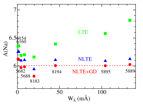
Figure 7: Na abundances derived from each of the 8 lines plotted against the equivalent widths, based on the results in Table 1. Squares, triangles, and circles correspond to the LTE abundances, the non-LTE abundances, and the final abundances (including both the non-LTE and gravity-darkening corrections), respectively. The horizontal dotted line indicates the average of the final abundances (6.01).

4.2 Composition characteristics of Li, Na, and K

According to Table 1, while potassium is only mildly subsolar ([K/H] $\simeq-0.2$) to an extent similar to sodium ($\sim-0.3$), lithium is more manifestly underabundant as [Li/H] $\simeq-0.6$. Therefore, we may conclude that the deficiency in Li is markedly different from that of Na and K, even considering the possible ambiguities of $\sim 0.2$ dex (cf. Sect. 3). How should we interpret these results? Do they have something to do with the element depletion (due to dust condensation) in interstellar gas and its accretion? Since the quantitative amount of such a depletion is different from case to case depending on the physical condition (e.g., see the variety of [Na/H]_ISM in Fig. 7 of Paunzen et al. 2002), it is not much meaningful to discuss the “absolute” values of [X/H] here. Rather, we should pay attention to their “relative” behaviors with each other or in comparison to those of various other elements.

The [X/H]_Vega values (those for Li, Na, and K are from this study, while those for other elements were taken from various literature) are plotted against the condensation temperature ($T_{\rm c}$) in Fig. 8 (filled circles), where the [X/H]_ISM results of typical interstellar gas in the direction of $\zeta$ Oph (taken from Table 5 of Savage & Sembach 1996; see also Fig. 4 therein) are also shown by open circles. The following characteristics can be recognized from this figure:
— (1) The [X/H]_Vega values, falling on a rather narrow range between $\sim-1$ and $\sim 0$, tend to decrease with $T_{\rm c}$, a qualitatively similar trend to that seen in [X/H]_ISM.
— (2) The run of [X/H]_Vega with $T_{\rm c}$ appears to be slightly discontinuous at $T_{\rm c}\sim 1000$ K (i.e., [X/H]${}_{\rm Vega}\sim-0.2$ to $-0.3$ at $T_{\rm c}\la 1000$ K and [X/H]${}_{\rm Vega}\sim-0.5$ to $-0.6$ at $T_{\rm c}\ga 1000$ K).
— (3) Interestingly, the decreasing [X/H]_ISM with $T_{\rm c}$ also shows a discontinuity around this critical $T_{\rm c}$ ($\sim 1000$ K) in the sense that the slope of $|d$[X/H]${}_{\rm ISM}/dT_{\rm c}|$ becomes evidently steeper on the $T_{\rm c}\ga 1000$ K side.
— (4) Specifically, the tendency of [Li/H]_Vega ($-0.6$) being more deficient than [Na/H]_Vega ($-0.3$) and [K/H]_Vega ($-0.2$) is qualitatively similar to just what is seen in ISM ([Li/H]${}_{\rm ISM}<$ [Na/H]${}_{\rm ISM}\simeq$ [K/H]_ISM).

All these observational facts may suggest the existence of some kind of connection between Vega’s photospheric abundances and those of interstellar cloud, which naturally implies that an accretion/contamination of interstellar gas is likely to be responsible (at least partly) for the abundance peculiarity of Vega, such as being proposed for explaining the $\lambda$ Boo phenomenon. This is the conclusion of this study.

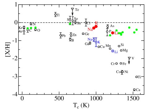
Figure 8: [X/H] values (relative abundances in comparison with the solar-system values of Grevesse & Noels 1993) of various elements plotted against the condensation temperature ($T_{\rm c}$). Open circles indicate the compositions of interstellar gas in the direction of $\zeta$ Oph (cool diffuse clouds), which were taken from Savage & Sembach (1996; cf. their Table 5 and Fig. 4). The [Na/H], [K/H], and [Li/H] for Vega derived in this study are shown by larger filled circles. Besides, Vega’s [X/H] values for other elements are plotted by smaller filled circles for a reference, which were taken from from various sources: Przybilla & Butler (2001) (for C, N, and O; cf. their Table 7); Takada-Hidai & Takeda (1996) (for S); Adelman & Gulliver (1990) (for Mg, Ca, Ti, Cr, Mn, Fe, and Ni); Qiu et al. (2001) (for Si and V). [Note. Since these literature [X/H] values of Vega were derived in a conventional manner based on classical atmospheric model, further corrections for the gravity-darkening effect ($\Delta_{\rm GD}$) are to be expected. According to Takeda et al. (2008), however, the extents of (negative) $\Delta_{\rm GD}$ (becoming appreciable only for very weak lines and for specific elements/stages) are only $\sim 0.2$ dex at most (e.g., Adelman & Gulliver’s [Ca/H] value derived from very weak Ca i lines had better be reduced by $\sim 0.2$ dex) while $\la 0.1$ dex in many typical cases, which are thus unlikely to cause any significant change in the general pattern of [X/H] shown here.]

Table 1: Atomic data, equivalent widths, and abundance results.

Species	RMT	$\lambda$	$\chi_{\rm low}$	$\log gf$	$W_{\lambda}$	$A_{\rm LTE}$	$\Delta_{\rm NLTE}$	$\Delta_{\rm GD}$	$A_{\rm NLTE+GD}$	[X/H]
		($\rm\AA$)	(eV)		(m$\rm\AA$)
Na i	1	5889.95	0.00	+0.12	133.3	6.82	$-$0.69	$-$0.09	6.03
Na i	1	5895.92	0.00	$-$0.18	104.2	6.58	$-$0.49	$-$0.08	6.01
Na i	4	8183.26	2.10	+0.22	19.7	6.16	$-$0.22	$-$0.12	5.82
Na i	4	8194.82	2.10	+0.52	45.1	6.39	$-$0.28	$-$0.10	6.01
Na i	5	6154.23	2.10	$-$1.56	0.8	6.36	$-$0.10	$-$0.12	6.13
Na i	5	6160.75	2.10	$-$1.26	1.6	6.36	$-$0.10	$-$0.14	6.12
Na i	6	5682.63	2.10	$-$0.67	4.3	6.19	$-$0.09	$-$0.13	5.97
Na i	6	5688.21	2.10	$-$0.37	8.4	6.20	$-$0.09	$-$0.12	5.99
									6.01	$-$0.30
K i	1	7664.91	0.00	+0.13	13.3	5.23	$-$0.28	$-$0.13	4.82
K i	1	7698.97	0.00	$-$0.17	10.7	5.42	$-$0.27	$-$0.14	5.01
									4.91	$-$0.22
Li i	1	6707.756	0.00	$-$0.43	0.7	3.15	$-$0.15	$-$0.26	2.74
		6707.768		$-$0.21
		6707.907		$-$0.93
		6707.908		$-$1.16
		6707.919		$-$0.71
		6707.920		$-$0.93
									2.74	$-$0.57

Following the atomic data of spectral lines (species, multiplet No., wavelength, lower excitation potential, and logarithmic $gf$ value) in columns 1–5, column 6 gives the measured equivalent width. The results of the abundance analysis are given in column 7 (LTE abundance; in the usual normalization of H=12.00), column 8 (non-LTE correction), column 9 (gravity-darkening correction), and column 10 (non-LTE as well as gravity-darkening corrected abundance). The finally adopted average abundance and the corresponding [X/H] value ($\equiv A_{\rm X}^{\rm Vega}-A_{\rm X}^{\odot}$) are also given at the bottom of the section (in italics; columns 10 and 11), where Grevesse & Noels’s (1993) values of 6.31 (Na), 3.31 (Li), and 5.13 (K) were used as the standard solar-system abundances ($A_{\rm X}^{\odot}$). Note that the analysis of $W_{\lambda}$(Li i 6708) was done by synthesizing the six component lines of ⁷Li (neglecting the contribution of ⁶Li; cf. Takeda & Kawanomoto 2005), while all the remaining lines of Na and K were analyzed by the single-line treatment as was done by Takeda et al. (2003; Na) and Takeda et al. (2002; K).

Appendix A Li abundance in $o$ Peg

The enhanced deficiency of Li (compared to Na and K) was an important key result in deriving the conclusion of this study (cf. Sect. 4.2), since we interpreted it as a manifestation of ISM compositions. In this connection, it may be worth mentioning another remarkable very sharp-lined A1 IV star, $o$ Peg, for which we could also get information of the Li abundance. As the only available measurement of the Li i 6708 line for early A-type stars thus far to our knowledge, Coupry & Burkhart (1992) derived $W_{\lambda}$(6708) = 1.3 m$\rm\AA$ for this star, which has atmospheric parameters ($T_{\rm eff}$ = 9650 K, $\log g=3.6$) quite similar to those of Vega except for its near-normal metallicity ([Fe/H] $\simeq+0.1$; Burkhart & Coupry 1991).

Now, their $W_{\lambda}$($o$ Peg) value twice as large as that of Vega (0.7 m$\rm\AA$) would raise the Li abundance by +0.3 dex. Furthermore, since any flat-bottomed shape has never been reported in the spectral lines of $o$ Peg (as we can confirm from the high-quality spectrum atlas of this star published by Gulliver, Adelman, & Friesen 2004), the application of the gravity-darkening correction ($\sim-0.3$ dex for Vega) may not be relevant here, which again leads to an increase of 0.3 dex. Hence, we have [Li/H]${}_{\rm oPeg}(\simeq$ [Li/H]_Vega + 0.6) $\sim 0.0$; an interesting result that the photospheric Li abundance of $o$ Peg almost coincides with that of the solar-system composition. This result, that [Li/H] (as well as [Fe/H]) is deficient/normal in Vega/$o$ Peg, may suggest that the mechanism responsible for producing the underabundance of these elements in Vega is irrelevant for $o$ Peg. Thus, according to our interpretation, $o$ Peg would not have suffered any pollution due to accretion of interstellar gas depleted in volatile elements of higher $T_{\rm c}$.

Yet, we had better keep in mind another possibility that the mechanism causing this Li deficiency in Vega might different from that of other metals. For example, this underabundance could be attributed to some process of envelope mixing (e.g., meridional circulation or shear-induced turbulence which are supposed to be more significant as a star rotates faster), because Li atoms are burned and destroyed when they are conveyed into the hot stellar interior ($T\ga 2.4\times 10^{6}$ K). Namely, since we know that Vega rotates rapidly (as fast as $v_{\rm e}\sim 200$ km s^-1) while $o$ Peg does not so much (at least the gravity-darkening effect is not so significant as in Vega), the underabundance of Li in the atmosphere of Vega might stem from the rotation-induced mixing (which is not expected for slowly rotating $o$ Peg). If this is the case, however, the rough similarity in the extent of deficiency in Li as well as other metals has to be regarded as a mere coincidence, which makes us feel this possibility as rather unlikely.

Appendix B Check for the final abundances: Complete spectrum synthesis

Our basic strategy for deriving the abundances of Na, K, and Li in Sect. 3 was as follows.
— (1) First, the $A_{\rm LTE}$ was derived from $W_{\lambda}^{\rm obs}$ based on the classical plane-parallel model atmosphere.
— (2) Next, the non-LTE correction ($\Delta_{\rm NLTE}$) was derived in the conventional way by using this classical model.
— (3) Then, the gravity darkening correction ($\Delta_{\rm GD}$) was evaluated from the line-intensification factor $W_{4}^{\rm LTE}/W_{0}^{\rm LTE}$ (where the abundance was so adjusted as to satisfy $W_{4}^{\rm LTE}\simeq W_{\lambda}^{\rm obs}$), which was computed by applying the CALSPEC program (Takeda et al. 2008) with the assumption of LTE to the gravity-darkened model 4 and the rigid-rotation model 0.
— (4) Finally, $A_{\rm NLTE+GD}$ was obtained as $A_{\rm LTE}+\Delta_{\rm NLTE}+\Delta_{\rm GD}$.

Actually, such a phased approach has a distinct merit of clarifying the importance/contribution of two different effects (the non-LTE effect and the gravity-darkening effect). Besides, from a practical point of view, the necessary amount of calculations to arrive at the final abundance solution (such that reproducing the observed spectrum) can be considerably saved.

However, there is some concern about whether such a step-by-step approach (treating the two effects separately) really yield sufficiently correct results, because both are actually related with each other (e.g., how does the largely variable non-LTE corrections over the gravity-darkened stellar surface differing in $T$ or $g$ play roles? How reliable is the gravity-darkening correction derived by neglecting the non-LTE effect?). Therefore, it may be worth checking the validity of the finally derived abundances ($A_{\rm NLTE+GD}$) by carrying out a complete spectrum synthesis including both NLTE and GD effects simultaneously. For this purpose, the CALSPEC program was modified so as to allow inclusion of the non-LTE departure coefficients (corresponding to the different conditions at each of the points over the gravity-darkened stellar surface), and the NLTE+GD profiles ($R_{4}^{\rm NLTE}$) were computed for each of the 9 lines (Na i 5890, 5896, 8183, 8195, 6154, 6161, 5683, 5688, K i 7664, 7699, and Li i 6708) by using the already known $A_{\rm NLTE+GD}$ values (6.03, 6.01, 5.82, 6.01, 6.13, 6.12, 5.97, 5.99, 4.82, 5.01, and 2.74, respectively). Such obtained $R_{4}^{\rm NLTE}$ profiles are depicted (in thick solid lines) in Fig. 9, where the relevant three kinds of line profiles [$R_{0}^{\rm NLTE}$ (thick dashed line), $R_{4}^{\rm LTE}$ (thin solid line), and $R_{0}^{\rm LTE}$ (thin dashed line)] are also shown for comparison.

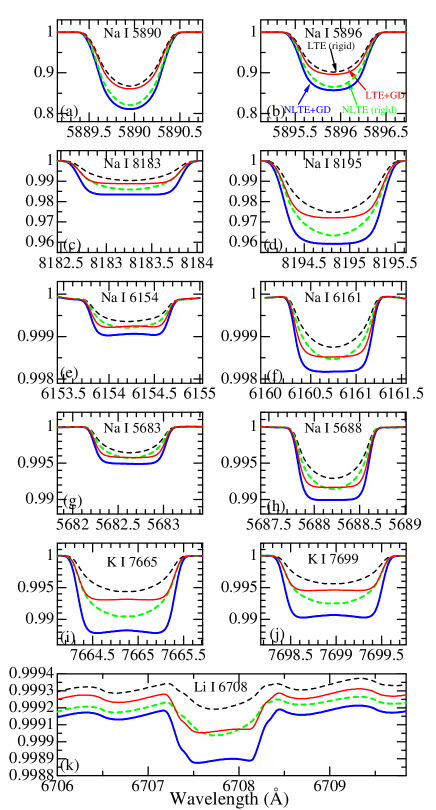
Figure 9: Theoretical profiles of the Na, K, and Li lines computed by the CALSPEC program (developed for synthesizing the flux spectrum for a given rotationally-distorted gravity-darkened stellar model; cf. Takeda et al. 2008), which has been modified to allow inclusion of the non-LTE effect. The $A_{\rm NLTE+GD}$ values given in Table 1 were assumed as the abundances for each of the lines. Results for the gravity-darkened model and the classical rigid-rotation model (model No. 4 and No. 0 in Takeda et al. 2008) are discriminated by the line type (solid and dashed lines, respectively), and those for NLTE and LTE are by the line thickness (thick and thin lines, respectively). As a result, four profiles are shown for each of the 9 lines: $R_{4}^{\rm NLTE}$ (thick solid line) $R_{0}^{\rm NLTE}$ (thick dashed line), $R_{4}^{\rm LTE}$ (thin solid line), and $R_{0}^{\rm LTE}$ (thin dashed line). Shown in the ordinate is the normalized flux divided by the theoretical (pure) continuum; therefore, the local continuum level sometimes turns out to be slightly less than unity because of the extended wings of H lines. (Note that the theoretical equivalent widths $W_{4}^{\rm NLTE}$ corresponding to $R_{4}^{\rm NLTE}$ profiles discussed in Appendix B were calculated with respect to the local continuum, i.e. the maximum level in the neighborhood of the line profiles, irrespective of the scales in the ordinate.) (a) Na i 5890, (b) Na i 5896, (c) Na i 8183, (d) Na i 8195, (e) Na i 6154, (f) Na i 6161, (g) Na i 5683, (h) Na i 5688, (i) K i 7665, (j) K i 7699, and (k) Li i 6708.

The resulting theoretical equivalent widths ($W_{4}^{\rm NLTE}$) computed by integrating $R_{4}^{\rm NLTE}(\lambda)$ are 129.7, 101.3, 18.4, 43.2, 0.8, 1.5, 4.0, 7.8, 12.8, 10.3, and 0.4 m$\rm\AA$ for these 9 lines, respectively. Comparing these values with the observed equivalent widths ($W_{\lambda}^{\rm obs}$) given in Table 1, we can see a satisfactory agreement between $W_{4}^{\rm NLTE}$ and $W_{\lambda}^{\rm obs}$ (typically to within several percent except for Li i 6708), by which we may conclude that the approach adopted in Sect. 3 is practically validated.

References

- (1) Adelman S.J., Gulliver A.F., 1990, ApJ, 348, 712
- (2) Andrievsky S.M., et al., 2002, A&A, 396, 641
- (3) Aufdenberg J.P., et al. 2006, ApJ, 645, 664 (erratum: 651, 617)
- (4) Baschek B., Slettebak A., 1988, A&A, 207, 102
- (5) Burkhart C., Coupry M.F., 1991, A&A, 249, 205
- (6) Castelli F., Kurucz R.L., 1994, A&A, 281, 817
- (7) Cayrel R. 1988, in Cayrel de Strobel G., Spite M., eds, The Impact of Very High S/N Spectroscopy on Stellar Physics, Proc. IAU Symp. 132, Kluwer, Dordrecht, p.345
- (8) Coupry M.F., Burkhart C., 1992, A&AS, 95, 41
- (9) Gerbaldi M., Faraggiana R., Castelli F., 1995, A&AS, 111, 1
- (10) Grevesse N., Noels A., 1993, in Prantzos N., Vangioni-Flam E., Cassé M., eds, Origin and evolution of the elements, Cambridge University Press, Cambridge, p.15
- (11) Gulliver A.F., Adelman S.J., & Friesen T.P. 2004, A&A, 413, 285,
- (12) Holweger H., Rentzsch-Holm I., 1995, A&A, 303, 819
- (13) Hunger K., 1955, Zs. Ap., 36, 42
- (14) Ilijić S., Rosandić M., Dominis D., Planinić M., Pavlovski K., 1998, Contrib. Astron. Obs. Skalnaté Pleso, 27, 467
- (15) Kamp I., Paunzen E., 2002, MNRAS, 335, L45
- (16) Kurucz R.L., 1993, Kurucz CD-ROM, No. 13, Harvard-Smithsonian Center for Astrophysics, http://kurucz.harvard.edu/cdroms.html
- (17) Paunzen E., 2004, in Zverko J., iovsk J., Adelman S.J., Weiss W.W., eds, The A-Star Puzzle, Proc. IAU Symp. 224, Cambridge University Press, Cambridge, p.443
- (18) Paunzen E., Iliev I.Kh., Kamp I., Barzova I.S., 2002, MNRAS, 336, 1030
- (19) Peterson D.M., et al. 2006, Nature, 440, 896
- (20) Przybilla N., Butler K., 2001, A&A, 379, 955
- (21) Qiu H.M., Zhao G., Chen Y.Q., Li Z.W., 2001, ApJ, 548, 953
- (22) Saffe C., Levato H., 2004, A&A, 418, 1083
- (23) Savage B.D., Sembach K.R., 1996, ARA&A, 34, 279
- (24) Strom S.E., Gingerich O., Strom K.M., 1966, ApJ, 146, 880
- (25) Stürenburg S., 1993, A&A, 277, 139
- (26) Takada-Hidai M., Takeda Y., 1996, PASJ, 48, 739
- (27) Takeda Y., Kawanomoto S., 2005, PASJ, 57, 45
- (28) Takeda Y., Takada-Hidai M., 1994, PASJ, 46, 395
- (29) Takeda Y., Kawanomoto S., Ohishi N., 2007, PASJ, 59, 245
- (30) Takeda Y., Kawanomoto S., Ohishi N., 2008, ApJ, 678, 446
- (31) Takeda Y., Zhao G., Chen Y.-Q., Qiu H.-M., Takada-Hidai M., 2002, PASJ, 54, 275
- (32) Takeda Y., Zhao G., Takada-Hidai M., Chen Y.-Q., Saito Y.-J., Zhang H.-W., 2003, ChJAA, 3, 316