Phase transition in site-diluted Josephson-junction arrays: A numerical study

Abstract

Intriguing effects produced by random percolative disorder in two-dimensional Josephson-junction arrays are studied by means of large-scale numerical simulations. Using dynamic scaling analysis, we evaluate critical temperatures and critical exponents in high accuracy. With the introduction of site-diluted disorder, the Kosterlitz-Thouless phase transition is eliminated and evolves into continuous phase transition with a power-law divergent correlation length. Moreover, genuine depinning transition and the related creep motion are studied, distinct types of creep motion for different disordered systems are observed. Our results not only are in good agreement with the recent experimental findings, but also shed some light on the relevant phase transitions.

I Introduction

Understanding the critical behavior of Josephson-junction arrays (JJA’s) with various disorders is always a challenging question and has been intensely studied in recent years harris –yunepl . However, the properties of different phases and various phase transitions are not well understood. Josephson-junction arrays gives an excellent realization to both two-dimensional (2D) XY model and granular High-$T_{c}$ superconductors lobb . As is well known that the pure JJA’s undergoes celebrated Kosterlitz-Thouless (KT) phase transition kt from the superconducting state to the normal state, this transition is driven by the unbinding of thermally created topological defects. When the disorder is introduced, the interplays between the periodic pinning potential caused by the discreteness of the arrays, the repulsive vortex-vortex interaction and the effects produced by the disorder provide a rich physical picture.

In diluted JJA’s, islands are randomly removed from the square lattice. Since it is a representative model for realizing the irregular JJA’s systems, how the percolation influences the physical properties of JJA’s has attracted considerable attention granato ; harris ; yun ; Benakli2 ; Granato2 . Harris $et$ $al$ introduced random percolative disorder into Nb-Au-Nb proximity-coupled junctions, the current-voltage ($I$-$V$) characteristics were measured and the results demonstrated that the only difference of the phase transition compared with that in ideal JJA’s system is the decrease of critical temperature, while the phase transition still belong to the KT-type with the disorder strength spanning from $p=0.7$ to $p=1.0$ (here $1-p$ is the fraction of diluted sites) harris . However, a recent experimental study by Yun $et$ $al$ showed that the KT-type phase transition in unfrustrated JJA’s was eliminated due to the introduction of site-diluted disorder yun . Therefore, the existence of the KT-type phase transition in site-diluted JJA’s remains a topic of controversy.

On the other hand, much attention has been paid to investigate the zero-temperature depinning transition and the related low-temperature creep motion both theoretically Nattermann ; Chauve ; Blatter and numerically Rosters ; luo ; olsson1 in a large variety of physical problems, such as charge density waves Nattermann , random-field Ising model Rosters , and flux lines in type-II superconductors luo ; olsson1 . Since the non-linear dynamic response is a striking aspect, there is increasing interest in these systems, especially in the flux lines of type-II superconductors luo ; olsson1 . In a recent numerical study on the three-dimensional glass states of flux lines, Arrhenius creep motion and non-Arrhenius creep motion were observed with strong collective pinning and weak collective pinning, respectively  luo .

In this work, we numerically investigate the finite-temperature phase transition in site-diluted JJA’s at different percolative disorders, the zero-temperature depinning transition and the low-temperature creep motion are also considered. The outline of this paper is as follows. Section II describes the model and the numerical method briefly. In section III, we present the simulation results, analyzing them by means of scaling analysis. Section IV gives a short summary of the main conclusions.

II Model and simulation method

JJA’s can be described by the 2D XY model on a simple square lattice, the Hamiltonian of which is olsson ; chenhu

$$H=-\sum\limits_{<i,j>}J_{ij}\cos(\phi_{i}-\phi_{j}-A_{ij}),$$ (1)

where the sum is over all nearest neighboring pairs on a 2D square lattice, $J_{ij}$ denotes the strength of Josephson coupling between site i and site j, $\phi_{i}$ specifies the phase of the superconducting order parameter on site i, and $A_{ij}=(2\pi/\Phi_{0})\int\mathbf{A}\cdot d\mathbf{l}$ is the integral of magnetic vector potential from site i to site j with $\Phi_{0}$ the flux quantum. The direct sum of $A_{ij}$ around an elementary plaquette is $2\pi f$, with $f$ the magnetic flux penetrating each plaquette produced by the uniformly applied field, measured in unit of $\Phi_{0}$. In this paper, $f=0$ and $f=2/5$ are in focus. The system sizes are selected as $128\times 128$ for $f=0$ and $100\times 100$ for $f=2/5$, the finite size effects in these sizes are negligible. Diluted sites are randomly selected, then the nearest four bonds of which are removed from the lattice. The same random-number seed is used to choose the diluted sites, the percolative threshold concentration is about $0.592(1)$ for both systems gebele .

The resistivity-shunted-junction (RSJ) dynamics is incorporated in the simulations, which can be described as chenhu ; chentang

$${\frac{\sigma\hbar}{2e}}\sum_{j}(\dot{\phi_{i}}-\dot{\phi_{j}})=-{\frac{\partial H}{\partial\phi_{i}}}+J_{{\rm ex},i}-\sum_{j}\eta_{ij},$$ (2)

where $\sigma$ is the normal conductivity, $J_{ex,i}$ refers to the external current, $\eta_{ij}$ denotes the thermal noise current with $<\eta_{ij}(t)>=0$ and $<\eta_{ij}(t)\eta_{ij}(t^{\prime})>=2\sigma k_{B}T\delta(t-t^{{}^{\prime}})$.

The fluctuating twist boundary condition is applied in the $xy$ plane to maintain the current, thus the new phase angle $\theta_{i}=\phi_{i}+r_{i}\cdot\Delta$ $(\Delta=(\triangle_{x},\triangle_{y})$ is the twist variable) is periodic in each direction. In this way, supercurrent between site i and site j is given by $J^{s}_{i\rightarrow j}=J_{ij}sin(\theta_{i}-\theta_{j}-A_{ij}-r_{ij}\cdot\Delta),$ and the dynamics of $\Delta_{\alpha}$ can be written as

$$\dot{\Delta}_{\alpha}=\frac{1}{L^{2}}\sum\limits_{<i,j>\alpha}[J_{i\rightarrow j}+\eta_{ij}]-I_{\alpha},$$ (3)

where $\alpha$ denotes the $x$ or $y$ direction, the voltage drop in $\alpha$ direction is $V=-L\dot{\Delta}_{\alpha}$. For convenience, units are taken as $2e=\hbar=J_{0}=\sigma=k_{B}=1$ in the following. Above equations can be solved efficiently by a pseudo-spectral algorithm due to the periodicity of phase in all directions. The time stepping is done using a second-order Runge-Kutta scheme with $\Delta t=0.05$. Our runs are typically $(4-8)\times 10^{7}$ time steps and the latter half time steps are for the measurements. The detailed procedure in the simulations was described in Ref. chenhu ; chentang . In this work, a uniform external current $I$ along $x$ direction is fed into the system.

Since RSJ simulations with direct numerical integrations of stochastic equations of motion are very time-consuming, it is practically difficult to perform any serious disorder averaging in the present rather large systems. Our results are based on one realization of disorder. For these very large samples, it is expected to exist a good self-averaging effect, which is confirmed by two additional simulations with different realizations of disorder. This point is also supported by a recent study of JJA’s by Um $et$ $al$ um , they confirmed that a well-converged disorder averaging for the measurement is not necessary, and well-converged data for large systems at a single disorder realization leads to a convincing result. In addition, simulations with different initial states are performed and the results are independent on the initial state we used. Actually, the hysteric phenomenon is usually negligible in previous RSJ dynamical simulations on JJA’s um ; Lim . For these reasons, the results from simulations with a unique initial state (random phases in this work) are accurate and then convincing.

III RESULTS AND DISCUSSION

III.1 Finite temperature phase transition

The $I$-$V$ characteristics are measured at various disorder strengths and temperatures. At each temperature, we try to probe the system at a current as low as possible. To check the method used in this work, we investigate the $I$-$V$ characteristics for $f=0,p=1.0$. As shown in Fig. 1(a), the slope of the $I$-$V$ curve in log-log plot at the transition temperature $T_{c}\approx 0.894$ is equal to 3, demonstrating that the $I$-$V$ index jumps from 3 to 1, in consistent with the well-known fact that the pure JJA’s experiences a KT-type phase transition at $T_{c}\approx 0.894$. Figs. 1(b) and (c) show the $I$-$V$ traces at different percolative disorders in unfrustrated JJA’s, while Fig. 1(d) for $f=2/5,p=0.65$. It is clear that, at lower temperatures, $R=V/I$ tends to zero as the current decreases, which follows that there is a true superconducting phase with zero linear resistivity.

It is crucial to use a powerful scaling method to analyze the $I$-$V$ characteristics. In this paper, we adopt the Fisher-Fisher-Huse (FFH) dynamic scaling method, which provides an excellent approach to analyze the superconducting phase transition FFH . If the properly scaled $I$-$V$ curves collapse onto two scaling curves above and bellow the transition temperature, a continuous superconducting phase transition is ensured. Such a method is widely used recently grt ; yang , the scaling form of which in 2D is

$$V=I\xi^{-z}\psi_{\pm}(I\xi),$$ (4)

where $\psi_{+(-)}(x)$ is the scaling function above (below) $T_{c}$, $z$ is the dynamic exponent, $\xi$ is the correlation length, and $V\sim I^{z+1}$ at $T=T_{c}$.

Assuming that the transition is continuous and characterized by the divergence of the characteristic length $\xi\sim|T-T_{c}|^{-\nu}$ and time scale $t\sim\xi^{z}$, FFH dynamic scaling takes the following form

$$(V/I)|T-T_{c}|^{-z\nu}=\psi_{\pm}(I|T-T_{c}|^{-\nu}).$$ (5)

On the other hand, a new scaling form is successfully adopted to certify a KT-type phase transition in JJA’s by holzer

$$(I/T)(I/V)^{1/z}=P_{\pm}(I\xi/T),$$ (6)

note that the Eq. (6) can be obtained directly from the FFH dynamic scaling form after some simple algebra. The correlation length of KT-type phase transition above $T_{c}$ is well defined as $\xi\sim e^{({c/|T-T_{c}|})^{1/2}}$ and Eq. (6) reads

$$(I/T)(I/V)^{1/z}=P_{+}(Ie^{({c/|T-T_{c}|})^{1/2}}/T).$$ (7)

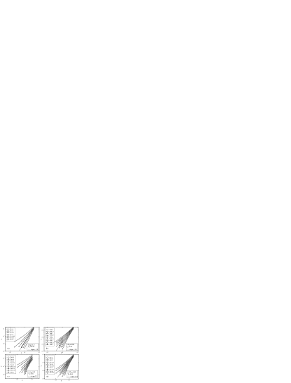
Figure 1: $I$-$V$ characteristics for different frustrations and percolative disorders. The dash lines are drawn to show where the phase transition occurs, the slopes of which are equal to $z+1$, z is the dynamic exponent. The transition temperature and dynamic exponent for (a) are well consistent with the well-known result, $i.$ $e.$, $T_{c}=0.894$, $z=2.0$, for (b),(c),(d) are well consistent with those determined by FFH dynamic scaling analysis. Solid lines are just guide to eyes.

As shown in Fig. 2, using $T_{c}=0.24\pm 0.01$, $z=1.2\pm 0.02$ and $\nu=1.0\pm 0.02$, we get an excellent collapse for $f=0,p=0.65$ according to equation (5). In addition, all the low-temperature $I$-$V$ curves can be fitted to $V\sim I$exp$(-(\alpha/I)^{\mu})$ with $\mu=0.9\sim 1.1$. These results certify a continuous superconducting phase with long-rang phase coherence. The critical temperature for such a strongly disordered system is very close to that in 2D gauge glass model ($T=0.22$) chen3 .

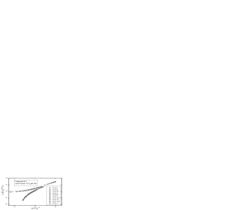
Figure 2: Dynamic scaling of $I$-$V$ data at various temperatures according to equation (5) for $f=0,p=0.65$.

For $f=0,p=0.86$, firstly, we still adopt the scaling form in equation (5) to investigate the $I$-$V$ characteristics. As displayed in Fig. 3, we get a good collapse for $T<T_{c}$ with $T_{c}=0.58\pm 0.01$, $z=2.0\pm 0.01$ and $\nu=1.4\pm 0.02$, demonstrating a superconducting phase with power-law divergent correlation for $T<T_{c}$. Note that the collapse is bad for $T>T_{c}$, indicating that the phase transition is not a completely non-KT-type one. Next, we use the scaling form in equation (7) to analyze the $I$-$V$ data above the critical temperature. Interestingly, using $T_{c}=0.58$ and $z=2.0$ determined above, a good collapse for $T>T_{c}$ is achieved, which is shown in Fig. 4. That is to say, the $I$-$V$ characteristics at $T<T_{c}$ are like those of a continuous phase transition with power-law divergent correlation length while at $T>T_{c}$ are like those of KT-type phase transition, which are well consistent with the recent experimental observations yun . Therefore, by the present model, we recover the phenomena in experiments and give some insight into the phase transition. More information on the low-temperature phase calls for further equilibrium Monte Carlo simulations as in Ref. Katzgraber .

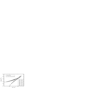
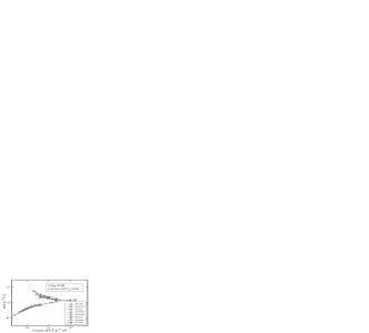
Figure 3: Dynamic scaling of $I$-$V$ data at various temperatures according to equation (5) for $f=0,p=0.86,T<T_{c}$. Solid lines are just guide to eyes.

Figure 4: Dynamic scaling of $I$-$V$ data at various temperatures according to equation (7) for $f=0,p=0.86,T>T_{c}$. Solid lines are just guide to eyes.

To make a comprehensive comparison with the experimental findings as in Ref. yun , we also investigated the finite-temperature phase transition in frustrated JJA’s ($f=2/5$) at a strong site-diluted disorder ($p=0.65$). As shown in Fig. 5, a superconducting phase transition with power-law divergent correlation is clearly observed. As is well known, non-KT-type phase transition in frustrated systems is a natural result. However, it is intriguing to see that in unfrustrated systems, one may ask what our results really imply and what is the mechanism for it. It has been revealed that in the presence of a strong random pinning which is produced by random site dilutions, a breaking of ergodicity due to large energy barrier against vortex motion may allow enough vortices to experience a non-KT-type continuous transition holme .

Figure 5: Dynamic scaling of $I$-$V$ data at various temperatures according to equation (5) for $f=2/5,p=0.65$.

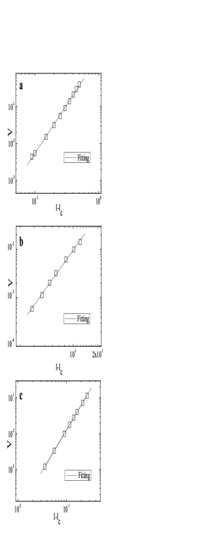
Figure 6: (a)$IV$ characteristics for $f=0,p=0.86$ with $I_{c}=0.302\pm 0.005$, $\beta=2.62\pm 0.1$. (b)$IV$ characteristics for $f=0,p=0.65$ with $I_{c}=0.039\pm 0.001$, $\beta=2.37\pm 0.1$. (c)$IV$ characteristics for $f=2/5,p=0.65$ with $I_{c}=0.035\pm 0.002$, $\beta=2.27\pm 0.05$

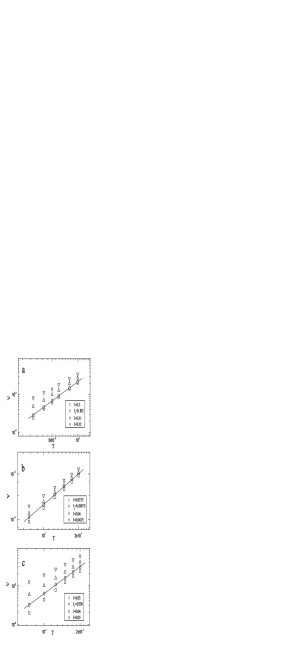
Figure 7: (a)LogV-LogT curves for $f=0,p=0.86$ in the vicinity of $I_{c}$ with $I_{c}=0.302\pm 0.001$, $1/\delta=1.688\pm 0.001$. (b)LogV-LogT curves for $f=0,p=0.65$ in the vicinity of $I_{c}$ with $I_{c}=0.03875\pm 0.0005$, $1/\delta=2.24\pm 0.02$. (c)LogV-LogT curves for $f=2/5,p=0.65$ in the vicinity of $I_{c}$ with $I_{c}=0.034\pm 0.001$, $1/\delta=2.29\pm 0.01$.

The systems considered in our work are site-diluted JJA’s, which are not the same as bond-diluted JJA’s in Ref. Granato2 ; Benakli2 . The difference is, in bond-diluted systems the diluted bonds are randomly removed, while in the site-diluted systems, the diluted sites are randomly selected, then the nearest four bonds around the selected sites are removed. Although the JJA’s in Ref. Granato2 ; Benakli2 and the present work are diluted in different ways, it is interesting to note that some of the obtained exponents are very close, possibly due to the similar disorder effect produced.

III.2 Depinning transition and creep motion

Next, we pay attention to the zero-temperature depinning transition and the related low-temperature creep motion for the typical site-diluted JJA’s systems mentioned above. Depinning can be described as a critical phenomenon with scaling law $V\sim(I-I_{c})^{\beta}$, demonstrating a transition from a pinned state below critical driving force $I_{c}$ to a sliding state above $I_{c}$. The $(I-I_{c}).vs.V$ traces at $T=0$ for $f=0,p=0.86$; $f=0,p=0.65$ and $f=2/5,p=0.65$ are displayed in Fig. 6, linear-fittings of $Log(I-I_{c}).vs.LogV$ curves are also shown as solid lines. As for $f=0,p=0.86$, the depinning exponent $\beta$ is determined to be $2.62\pm 0.1$ and the critical current $I_{c}$ is $0.302\pm 0.005$, while for the cases $f=0,p=0.65$ and $f=2/5,p=0.65$, the depinning exponents are evaluated to be $2.37\pm 0.1$ and $2.27\pm 0.05$ with the critical currents $I_{c}=0.039\pm 0.001$ and $I_{c}=0.035\pm 0.002$, respectively.

When the temperature increases slightly, creep motions can be observed. In the low-temperature regime, the $I$-$V$ traces are rounded near the zero-temperature critical current due to thermal fluctuations. Fisher first suggested to map such a phenomenon for the ferromagnet in magnetic field where the second-order phase transition occurs  fisher22 . This mapping was then extended to the random-field Ising model  Rosters and the flux lines in type-II superconductors  luo . For the flux lines in type-II superconductors, if the voltage is identified as the order parameter, the current and the temperature are taken as the inverse temperature and the field respectively, analogous to the second-order phase transition in the ferromagnet, the voltage, current and the temperature will satisfy the following scaling ansatz  luo ; chen3

$$V(T,I)=T^{1/\delta}S[(1-I_{c}/I)T^{-1/\beta\delta}].$$ (8)

The relation $V(T,I=I_{c})=S(0)T^{1/\delta}$ can be easily derived at $I=I_{c}$, by which the critical current $I_{c}$ and the critical exponent $\delta$ can be determined through the linear fitting of the $LogT-LogV$ curve at $I_{c}$. The $LogT-LogV$ curves are plotted in Fig. 7(a) for $f=0,p=0.86$. We can observe that the critical current is between 0.3 and 0.32. In order to locate the critical current precisely, we calculate other values of voltage at current within (0.3,0.32) with a current step 0.01 by quadratic interpolation chen3 . Deviation of the $T$-$V$ curves from the power law is calculated as the square deviations $SD=\sum[V(T)-y(T)]^{2}$ between the temperature range we calculated, here the functions $y(T)=C1T^{-C2}$ are obtained by linear fitting of the $LogT-LogV$ curves. The current at which the $SD$ is minimum is defined as the critical current. The critical current is then determined to be $0.302\pm 0.001$. Simultaneously, we obtain the exponent $1/\delta=1.688\pm 0.001$ from the slope of $LogT-logV$ curve at $I_{c}=0.302$. The similar method is applied to investigate the cases $f=0,p=0.65$ and $f=2/5,p=0.65$. As shown in Figs. 7 (b) and (c), the critical current $I_{c}$ and critical exponent $1/\delta$ for $f=0,p=0.65$ are determined to be $0.03875\pm 0.0005$, $2.24\pm 0.02$ respectively, for $f=2/5,p=0.65$, the result is $I_{c}=0.034\pm 0.001$, $1/\delta=2.29\pm 0.01$.

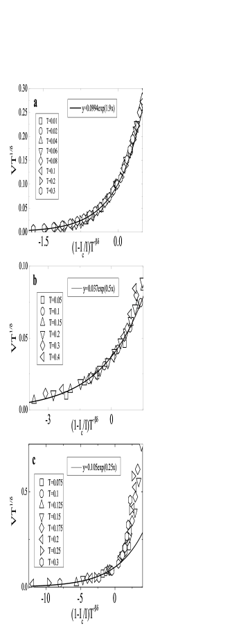
Figure 8: (a) Scaling plot for $f=0,p=0.86$ with $I_{c}=0.302$, $1/\delta=1.688$ and $\beta\delta=1.55$. (b) Scaling plot for $f=0,p=0.65$ with $I_{c}=0.03875$, $1/\delta=2.24$ and $\beta\delta\approx 1.0$. (c)Scaling plot for $f=2/5,p=0.65$ with $I_{c}=0.034$, $1/\delta=2.29$ and $\beta\delta\approx 1.0$.

We then draw the scaling plots according to Eq. 8. Using the one parameter tuning of $\beta$, we get the best collapses of data to a single scaling curve with $\beta=2.61\pm 0.02$ and $2.28\pm 0.02$ for $f=0,p=0.86$ and $f=0,p=0.65$ in the regime $I\leq I_{c}$, respectively, which are shown in Figs. 8(a) and (b). For $f=0,p=0.86$, this curve can be fitted by $S(x)=0.0994exp(1.9x)$, combined with the relation $\beta\delta=1.55$, suggesting a non-Arrhenius creep motion. However, for the strongly site-diluted system with $f=0,p=0.65$, the scaling curve can be fitted by $S(x)=0.037exp(0.5x)$, combined with the relation $\beta\delta\approx 1.0$, indicative of an Arrhenius creep motion. Interestingly, as displayed in Fig. 8(c) for $f=2/5,p=0.65$, the exponent $\beta$ is fitted to be $2.30\pm 0.02$, which yields $\beta\delta\approx 1.0$. The scaling curve in the regime $I\leq I_{c}$ can be fitted by $S(x)=0.105exp(0.25x)$. These two combined facts suggest an Arrhenius creep motion in this case.

It is worthwhile to note that both the finite-temperature phase transition and the creep motion for strongly disordered JJA’s ($p=0.65$) with and without frustration are very similar. The $I$-$V$ curves in low temperature for all three cases can be described by $V\propto T^{1/\delta}exp[A(1-I_{c}/I)/T^{\beta\delta}]$, which is just one of the main characteristics of glass phases luo ; chen3 . While the $I$-$V$ traces for KT-type phases can be fitted to $V\propto I^{a}$. Therefore, we have provided another evidence for the existence of non-KT-type phases in the low-temperature regime for these three cases ($f=0,p=0.86;f=0,p=0.65;f=2/5,p=0.65$).

IV SUMMARY

To explore the properties of various phase transitions in site-diluted JJA’s, we have performed large scale simulations at two typical percolative strengths $p=0.86$ and $p=0.65$ as in a recent experimental work yun . The RSJ dynamics was incorporated in our work, from which we measured the $I$-$V$ characteristics at different temperatures. The critical temperature of the finite-temperature phase transition was found to decrease as the diluted sites increase. For $f=0,p=0.86$, the phase transition is the combination of a KT-type transition and a continuous transition with power-law divergent correlation length. At strong percolative disorder ($p=0.65$), the KT-type phase transition in pure JJA’s is changed into a completely non-KT-type phase transition, moreover, the finite-temperature phase transition for frustrated JJA’s is similar to that in unfrustrated JJA’s. All the obtained dynamic exponents $z=a-1$, with $a$ the $I$-$V$ index at the critical temperature, and all the static exponents fall in the range of $\nu=(1.0,2.0)$ usually observed at vortex-glass transitions experimentally. Following table summarizes the critical temperatures at different frustrations and disorder strengths.

Table 1: Summary of $T_{c}$.

	f=0	f=2/5
p=0.95	0.85(2)	0.16(2)
p=0.86	0.58(1)	0.13(1)
p=0.7	0.27(2)	0.12(1)
p=0.65	0.24(1)	0.14(1)

In a recent experiment, Yun et al yun suggested a non-KT-type phase transition in unfrustrated JJA’s with site-diluted disorder for the first time, however the nature of these phase transitions and various phases is still in an intensive debate. Our results not only recover the recent experimental findings yun , but also shed some light on the various phases. Non-KT-type finite-temperature phase transition in site-diluted JJA’s was confirmed by the scaling analysis. The different divergent correlations at various disorder strengths were suggested, the critical exponents were evaluated in high accuracy, which are crucial for understanding such a critical phenomenon. Furthermore, the results in this paper are not only useful for understanding the site-diluted systems, but also useful for understanding the whole class of disordered JJA’s. For instance, the combination of two different phase transitions may exist in other disordered JJA’s systems.

In addition, the zero-temperature depinning transition and the low-temperature creep motion are also touched. It is demonstrated by the scaling analysis that the creep law for $f=0,p=0.86$ is non-Arrhenius type while those for $f=0,p=0.65$ and $f=2/5,p=0.65$ belong to the Arrhenius type. The evidence of non-KT-type phase transition can also be provided by this scaling analysis. It is interesting to note that the non-Arrhenius type creep law for weak disorder ($f=0,p=0.86$) is similar to that in three-dimensional flux lines with a weak collective pinning luo . The product of the two exponents $1.55$ is also very close to $3/2$ determined in Ref.luo . For $f=0,p=0.65$ and $f=2/5,p=0.65$, the observed Arrhenius type creep law is also similar to that in the glass states of flux lines with a strong collective pinning as in Ref. luo . Future experimental work is needed to clarify this observation.

V ACKNOWLEDGEMENTS

This work was supported by National Natural Science Foundation of China under Grant Nos. 10774128, PCSIRT (Grant No. IRT0754) in University in China, National Basic Research Program of China (Grant Nos. 2006CB601003 and 2009CB929104), and Zhejiang Provincial Natural Science Foundation under Grant No. Z7080203.

^† Corresponding author. Email:qhchen@zju.edu.cn

References

- (1) D. C. Harris, S. T. Herbert, D. Stroud and J. C. Garland, Phys. Rev. Lett. 67, 3606 (1991).
- (2) E. Granato and D. Domínguez, Phys. Rev. B 56, 14671 (1997).
- (3) M. Benakli and E. Granato, S. R. Shenoy and M. Gabay, Phys. Rev. B 57, 10314 (1998).
- (4) E . Granato and D. Dominguez, Phys. Rev. B 63, 094507 (2001).
- (5) Y. J. Yun, I. C. Baek and M. Y. Choi, Phys. Rev. Lett. 89, 037004 (2002).
- (6) E. Granto and D. Dominguez, Phys. Rev. B 71, 094521 (2005).
- (7) J. S. Lim, M. Y. Choi, B. J. Kim and J. Choi, Phys. Rev. B 71, 100505R (2005).
- (8) J. Um, B. J. Kim, P. Minnhagen, M. Y. Choi and S. I. Lee, Phys. Rev. B 74, 094516 (2006).
- (9) Y. J. Yun, I. C. Baek and M. Y. Choi, Phys. Rev. Lett. 97, 215701 (2006).
- (10) Y. J. Yun, I. C. Baek and M. Y. Choi, Europhys. Lett. 76, 271 (2006).
- (11) C. J. Lobb, D. W. Abraham and M. Tinkham, Phys. Rev. B 27, 150 (1983); M. Prester, Phys. Rev. B 54, 606 (1996).
- (12) J. M. Kosterlitz and D. J. Thouless, J.Phys.C 6, 1181 (1973); J. M. Kosterlitz, J. Phys. C 7, 1046 (1974); V. L. Berezinskii, Sov. Phys. - JETP, 34,610 (1972); V. L. Berezinskii, Zh. Eksp. Teor. Fiz. 61,1144 (1973).
- (13) T. Nattermann, Phys. Rev. Lett. 64, 2454 (1990).
- (14) P. Chauve, T. Giamarchi and P. L. Doussal, Phys. Rev. B. 62, 6241 (2000).
- (15) M. Müller, D. A. Gorokhov and G. Blatter, Phys. Rev. B. 63, 184305 (2001).
- (16) L. Rosters, A. Hucht, S. Lübeck, U. Nowak and K. D. Usadel, Phys. Rev. E. 60, 5202 (1999).
- (17) M. B. Luo and X. Hu, Phys. Rev. Lett. 98, 267002 (2007).
- (18) P. Olsson, Phys. Rev. Lett. 98, 097001 (2007); Q. H. Chen, Phys. Rev. B 78, 104501 (2008).
- (19) P. Olsson and S. Teitel, Phys. Rev. Lett. 87, 137001 (2001).
- (20) Q. H. Chen and X. Hu, Phys. Rev. Lett. 90, 117005 (2003); Q. H. Chen and X. Hu, Phys. Rev. B 75, 064504 (2007).
- (21) T. Gebele, J. Phys. A: Math. Gen. 17, L51(1984); Y. Laroyer and E. Pommiers, Phys.Rev.B 50, 2795 (1994).
- (22) Q. H. Chen and L. H. Tang, Phys. Rev. Lett. 87, 067001 (2001); L. H. Tang and Q. H. Chen, Phys. Rev. B 67, 024508 (2003).
- (23) D. S. Fisher, M. P. A. Fisher and D. A. Huse, Phys. Rev. B 43, 130 (1991).
- (24) H. Yang, Y. Jia, L. Shan, Y. Z. Zhang, H. H. Wen, C. G. Zhuang, Z. K. Liu, Q. Li, Y. Cui and X. X. Xi, Phys. Rev. B 76, 134513 (2007).
- (25) J. Holzer, R. S. Newrock, C. J. Lobb, T. Aouaroun and S. T. Herbert, Phys. Rev. B 63, 184508 (2001).
- (26) Q. H. Chen, J. P. Lv, H. Liu, Phys. Rev. B 78, 054519 (2008).
- (27) H. G. Katzgraber, Phys. Rev. B 67, 180402R (2003); H. G. Katzgraber and A. P. Young, Phys. Rev. B 66 224507 (2002).
- (28) P. Holme and P. Olsson, Europhys. Lett. 60 439 (2002).
- (29) D. S. Fisher, Phys. Rev. Lett. 50, 1486 (1983); Phys. Rev. B 31, 1396 (1985).