Accurate estimator of correlations between asynchronous signals

Abstract

The estimation of the correlation between time series is often hampered by the asynchronicity of the signals. Cumulating data within a time window suppresses this source of noise but weakens the statistics. We present a method to estimate correlations without applying long time windows. We decompose the correlations of data cumulated over a long window using decay of lagged correlations as calculated from short window data. This increases the accuracy of the estimated correlation significantly and decreases the necessary efforts of calculations both in real and computer experiments.

1 Introduction

Correlations between time series are fundamental for understanding and interpreting stochastic processes. Very often the time between the signals of a series is distributed in an uneven fashion, causing asynchronicity of the compared series.

Correlations between asynchronous signals can be of great importance in several areas. An important example is the case of neutron activation analysis [1]. These experiments are used for non-destructive testing of materials in order to determine the concentration of their constituents. In the analysis the specimen is bombarded by neutrons coming from a source, causing the elements to form radioactive isotopes, and from the spectra of the emissions of the radioactive sample, the concentration of the elements can be determined. Since the radiation appears together for all kinds of atoms, different elements are going to radiate in a correlated but asynchronous way [1, 2].

Another example can be taken from materials science or seismology. Mechanical failures can be tested by their wave radiation and it is crucial to know if the signals measured by different sensors are correlated [3]. Obviously, the analysis involves the handling of asynchronous signals.

Correlations of returns of different companies are fundamental input data for portfolio optimisation. As the transactions are asynchronous, the correlations measured on short time scale are significantly reduced, which is called the Epps effect [4].

From theoretical point of view continuous time random walks [5] can be mentioned, that can be used to describe a broad range of processes from transport in disordered solids [6] to finance [7]. Correlated continuous random walks produce asynchronous time series.

When computing the Pearson correlation coefficient of two stationary signals we often have to face an important problem: The correlation measure is designed to determine the grade of co-movements of synchronous observations, while the signals are asynchronous. The usual way to handle this problem is to cumulate data over a time window $\Delta t$ and look for the correlations between these binned data. In order to approach the asymptotic, proper value of the correlation coefficient, $\Delta t$ should be much larger than the scale of asynchronicity. However, this leads to the reduction of the statistics, consequently it makes the estimates inaccurate. On the other hand, for short $\Delta t$ the noise due to asynchronicity may reduce the measured correlations significantly.

It has been suggested to use measures of correlation other than the Pearson coefficient to overcome the problem of asynchronicity. Ref. [8] presents a method of measuring covariance based on Fourier series analysis of data. This method has been applied by Refs. [9, 10] in the study of financial correlations. While the Fourier method is indeed somewhat less sensitive to asynchronicity, the problem cannot be eliminated by its use. Refs. [11] propose a new estimator of the covariance of two diffusion processes that are observed only at discrete times in a non-synchronous manner. Their estimator uses all available data and does not require synchronization of observations, however in the presence of noise it becomes inconsistent and its variance diverges. A good comparison of several covariance estimators can be found in Refs [12, 13].

In this paper we describe an estimator of the Pearson correlation coefficient for correlated, asynchronous pairs of data based on an appropriate decomposition of the expression for the correlation coefficient for large $\Delta t$ by using the value of the coefficient for small time window and decay of lagged correlations. The latter can be calculated from the good statistics high resolution data. We applied the decomposition scheme already to explain [14] the Epps effect [4]. Here we show how it can be used to accurately estimate the asymptotic correlation coefficients.

The paper is organized as follows: In Section 2 we review the decomposition of correlations. Section 3 contains the description of our method together with some demonstrative results. In Section 4 we apply the method to real data. We end the paper with a short summary in Section 5.

2 Decomposition of correlations

Let us consider a system, where discrete stationary signals arrive from two different sources (A and B) at different time instances resulting in two correlated time series. We count the hits arriving, and denote their cumulative number measured from a reference time $t=0$ at time $t$ by $c^{A}(t)$ and $c^{B}(t)$ respectively.

We are interested in the correlation between the number of hits arriving to our sensor in a certain time window, thus the change in $c^{A}$ and $c^{B}$. This will be denoted by

$$r^{A}_{\Delta t}(t)=c^{A}(t)-c^{A}(t-\Delta t).$$ (1)

The general Pearson correlation measure with time lag $\tau$ is defined by

$$C_{\Delta t}^{A/B}(\tau)=\frac{\left\langle\Delta r_{\Delta t}^{A}(t)\Delta r_{\Delta t}^{B}(t+\tau)\right\rangle}{\sigma^{A}\sigma^{B}},$$ (2)

where $\Delta r_{\Delta t}(t)$ is the deviation of $r_{\Delta t}(t)$ from its mean,

$$\left\langle\Delta r_{\Delta t}^{A}(t)\Delta r_{\Delta t}^{B}(t+\tau)\right\rangle=$$

$$=\frac{1}{N}\sum_{i=1}^{N}\Delta r_{\Delta t}^{A}(i\Delta t)\Delta r_{\Delta t}^{B}(i\Delta t+\tau),$$ (3)

with $N=[(T-\tau)/\Delta t]$ and $\sigma^{A}$ ($\sigma^{B}$) is the standard deviation of $r_{\Delta t}^{A}$ ($r_{\Delta t}^{B}$).

We use $\langle\dots\rangle$ for denoting time average. The equal-time correlation coefficient is naturally: $\rho_{\Delta t}^{A/B}\equiv C_{\Delta t}^{A/B}(\tau=0)$.

As we can see, already by the definition, the length of the time window, i.e. the value of $\Delta t$ plays a major role in measuring the correlation.

Assuming $\Delta t=n\Delta t_{0}$ with $n$ being a positive integer, we can deduce the following relationship between correlations on the two different time scales

$$\rho_{\Delta t}^{A/B}=\Bigg{(}\sum_{x=-n+1}^{n-1}\left(n-|x|\right)\left\langle r_{\Delta t_{0}}^{A}(t)r_{\Delta t_{0}}^{B}(t+x\Delta t_{0})\right\rangle-n^{2}\left\langle r^{A}_{\Delta t_{0}}(t)\right\rangle\left\langle r^{B}_{\Delta t_{0}}(t)\right\rangle\Bigg{)}\times$$

$$\Bigg{(}\sum_{x=-n+1}^{n-1}\left(n-|x|\right)\left\langle r_{\Delta t_{0}}^{A}(t)r_{\Delta t_{0}}^{A}(t+x\Delta t_{0})\right\rangle-n^{2}\left\langle r^{A}_{\Delta t_{0}}(t)\right\rangle^{2}\Bigg{)}^{-1/2}\times$$

$$\Bigg{(}\sum_{x=-n+1}^{n-1}\left(n-|x|\right)\left\langle r_{\Delta t_{0}}^{B}(t)r_{\Delta t_{0}}^{B}(t+x\Delta t_{0})\right\rangle-n^{2}\left\langle r^{B}_{\Delta t_{0}}(t)\right\rangle^{2}\Bigg{)}^{-1/2}.$$ (4)

Details on the deduction of Equation 2 can be found in the Appendix. It is plausible to set $\Delta t_{0}$ as the shortest meaningful time scale in the system, that has to be chosen with the actual problem in mind.

This decomposition can be used to accurately estimate correlations by using high resolution, i.e., good statistics data.

3 Method

Expression (2) enables to calculate the correlation coefficient for any sampling time scale, $\Delta t$, by knowing the coefficient on a shorter sampling time scale, $\Delta t_{0}$, and the decay of lagged correlations on the same shorter sampling time scale (given that $\Delta t$ is multiple of $\Delta t_{0}$).

The method we would like to propose relies on this decomposition of correlations.

We suggest the following procedure. Data should be binned with a small $\Delta t_{0}$ such that a good statistics is achieved, irrespective of the fact that noise due to asynchronicity may be considerable. Then the correlation functions and the decay of lagged correlations should be calculated using these data (of course the calculated correlation can be expected to be too small). Plugging in these quantities into Equation (2) with a large enough $\Delta t$ we obtain a good estimate for the proper correlation. Using different values of $\Delta t$ an extrapolation to the proper, asymptotic correlation coefficient is possible.

We demonstrate the method in more details in this section. We use correlated random walks and show that in case of directly measuring the correlations in large $\Delta t$ time windows we need very long time series in order to have a good estimate for correlations. When using the decomposition method, we use high resolution data and thus can achieve an estimate for the correlations with the same accuracy from a dataset of much shorter time span.

3.1 Demonstration

We construct correlated asynchronous time series in the following way: As a first step we generate a core random walk with unit steps up or down in each second:

$$W(t)=W(t-1)+\varepsilon(t),$$ (5)

where $\varepsilon(t)$ is $\pm 1$ with equal probability. Second we sample the random walk, $W(t)$, twice independently with sampling time intervals drawn from some distribution. This way we simulate asynchronicity by non-simultaneously sampling our generated data. A snapshot of the random walks can be seen in Figure 1.

\psfrag{W(t)}[2.5][0]{W(t)}\psfrag{cA(t)}[2.5][0]{$c^{A}(t)$}\psfrag{cB(t)}[2.5][0]{$c^{B}(t)$}\includegraphics[angle={-90},width=325.215pt]{example_of_model_exp.ps}

Figure 1: (Color online) Illustration of the asynchronous sampling, as introduced in [14]. The original random walk is shown with lines (black), the two sampled series with triangles and line (red) and dots and line (blue).

Below we present results first for exponentially distributed sampling intervals between steps and second for the sampling intervals between steps being drawn from a Weibull distribution. We study the correlation between the changes in the position of the two random walkers.

3.1.1 Exponential sampling intervals

We generate 50 pairs of time series, as described above, with sampling intervals

between consecutive changes from the distribution:

$$\mathbb{P}(y)=\Bigg{\{}\begin{array}[]{ll}\lambda e^{-\lambda y}&\textrm{if }y\geq 0\\ 0&y<0\end{array}$$ (8)

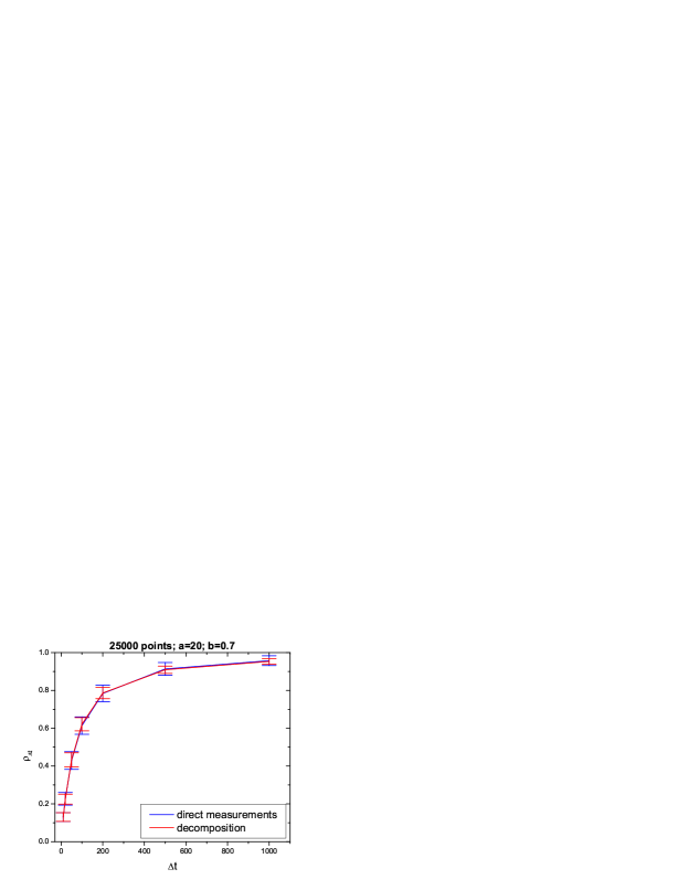
with parameter $\lambda=1/60$. Each time series has a length of 25000 time steps. Naturally, since the time series are finite, the correlation coefficients that we measure will have errors. In Figure 2 we show the results for the correlation coefficients on different time scales, where the shortest time scale used was $\Delta t_{0}=10$.

Figure 2: (Color online) Comparison of the directly measured correlation coefficients and the coefficients determined through the decomposition method in case of exponentially distributed sampling intervals. In blue we show the average and the standard deviation of the direct measurements computed over the ensemble of 50 time series pairs. In red we show the average and the standard deviation obtained by the decomposition method, computed over the ensemble of 50 time series pairs.

In blue we show the average of the direct measurements, taken over 50 points. The errorbars show the standard deviation of the points. In red we show the average result obtained by the decomposition method using Equation 2, taken over 50 points, with their standard deviation as errorbars. As we can see there is a significant difference between the errors of the two measurements, while their means are very near to each other. In general, the error of measurements goes as $\sigma/\sqrt{N}$, where $\sigma$ is the standard deviation of the distribution of results and $N$ is the number of data points. The ratio of the standard deviations at $\Delta t=1000$ in Figure 2 is close to 3. This means that in order to obtain the same precision from direct measurements as from the decomposition method, we need roughly one order of magnitude more data points.

Generally, one is interested in the asymptotic value of the correlations, i.e. in the limit of $\rho_{\Delta t\to\infty}$. As we can see, even for the numerically generated data, determining the correlation for the scale of $\Delta t=1000$ we still get a correlation different from the underlying asymptotic correlation, that is 1. A possible way to determine the asymptotic correlation value is using some extrapolation method.

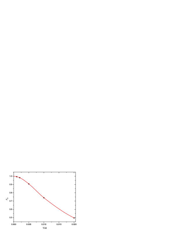
We demonstrate that applying a simple extrapolation method for the generated data we can determine the exact underlying correlation with very good accuracy. Since we are interested in the $\Delta t\to\infty$ value, we use the plot of $\rho_{\Delta t}$ as a function of $1/\Delta t$ for the extrapolation. Figure 3 shows the correlation points and the curve determined by piecewise Cubic Hermite Interpolation method. The extrapolated curve intercepts the y-axis at the value of 1.002, which is very close to the actual asymptotic correlation value, with an error around $0.2\%$.

Figure 3: (Color online) The correlation as a function of $1/\Delta t$ for the exponentially distributed sampling intervals. The circles show the correlations determined using the decomposition method, and the (red) curve is the piecewise Cubic Hermite Interpolation of the correlation values. The extrapolation gives an asymptotic correlation value of 1.002, very close to the actual underlying value, that is 1.

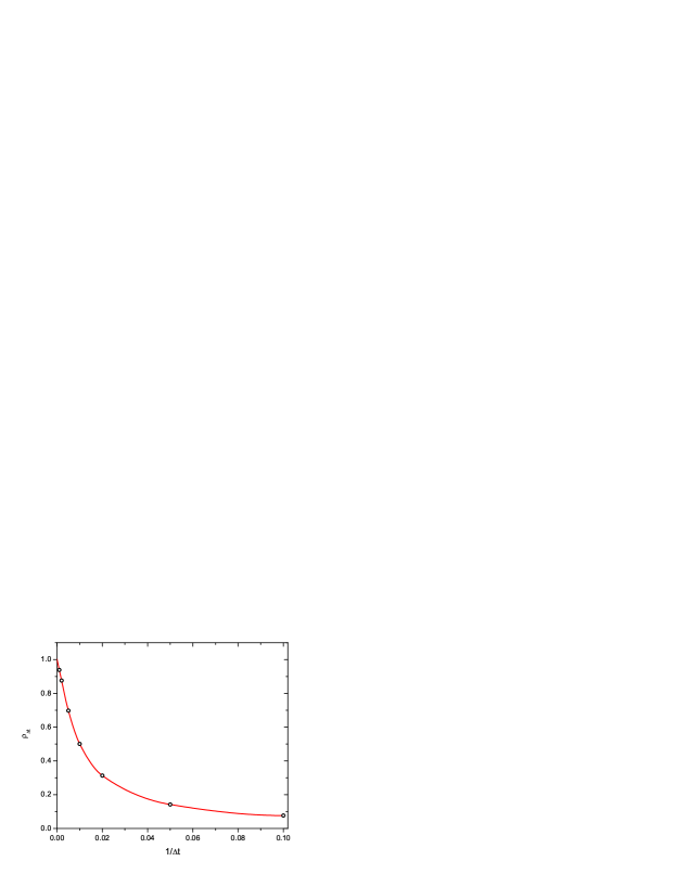
We studied the effect of the errors of the two methods on the accuracy of the extrapolated value of the correlation coefficient. Applying a piecewise Cubic Hermite Interpolation to the endpoints of the error bars, we find that the extrapolated value of the asymptotic correlations using direct measurements falls between 0.979 and 1.035, while the value for the decomposition method falls between 0.998 and 1.005, indicating a factor of 8 improvement in the precision.

3.1.2 Weibull sampling intervals

In order to demonstrate the power of the method for a non Poisson process we generate 50 pairs of time series, as described above, with sampling intervals between consecutive changes generated from a Weibull distribution:

$$\mathbb{P}(y)=\Bigg{\{}\begin{array}[]{ll}\frac{b}{a}(\frac{y}{a})^{b-1}e^{-(y/a)^{b}}&\textrm{if }y\geq 0\\ 0&y<0\end{array}$$ (11)

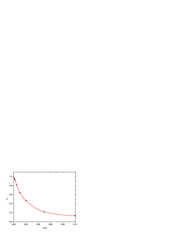
with parameters $a=20$ and $b=0.7$. Again each time series has a length of 25000 time steps and the directly measured correlation values have large variance. In Figure 4 we show the results for the correlation coefficients on different time scales, again with $\Delta t_{0}=10$.

Figure 4: (Color online) Comparison of the directly measured correlation coefficients and the coefficients determined through the decomposition method in case of Weibull distributed sampling intervals. In blue we show the average and the standard deviation of the direct measurements computed over the ensemble of 50 time series pairs. In red we show the average and the standard deviation obtained by the decomposition method, computed over the ensemble of 50 time series pairs.

The Figure shows that we get a better estimate of the means from the decomposition formula than from direct measurements. In this case the ratio of the standard deviations at $\Delta t=1000$ is close to 2. The same improvement is obtained for the precision of the extrapolated asymptotic correlation coefficients. The extrapolation of the asymptotic coefficient can be seen in Figure 5.

The two above examples on generated time series show that using our method and estimating the correlation coefficient between asynchronous signals from the high frequency data leads to much smaller variation of the results than in case of direct measurement of correlations on lower frequency data.

Figure 5: (Color online) The correlation as a function of $1/\Delta t$ for the Weibull distributed sampling intervals. The circles show the correlations determined using the decomposition method, and the (red) curve is the piecewise Cubic Hermite Interpolation of the correlation values. The extrapolation gives an asymptotic correlation value of 0.992, very close to the actual underlying value, that is 1.

3.2 Decay functions

As we can see from Equation (2) a subtle point of the correlation estimation is the measurement of the decay of lagged correlations on the short ($\Delta t_{0}$) time scale, that we will call decay functions. There are three decay functions we have to measure: $\left\langle r_{\Delta t_{0}}^{A}(t)r_{\Delta t_{0}}^{A}(t+x\Delta t_{0})\right\rangle$, $\left\langle r_{\Delta t_{0}}^{B}(t)r_{\Delta t_{0}}^{B}(t+x\Delta t_{0})\right\rangle$ and $\left\langle r_{\Delta t_{0}}^{A}(t)r_{\Delta t_{0}}^{B}(t+x\Delta t_{0})\right\rangle$. To have good estimation of the asymptotic correlation value, one has to have precise measurements of these decay functions.

In the above examples we had random walks as underlying processes, thus by definition the autocorrelations are delta functions. However, because of the asynchronous sampling, the cross-correlation is being smeared out and instead of a delta function we have finite decay of the cross-correlation. These cases are simple from the point of view of the decay functions. To demonstrate that in case of more complicated vanishing decay functions the decomposition can still give a good estimation of the asymptotic correlation, we consider the following time series. We generate a persistent random walk [15, 16], ie. a walk, where the probability, $\alpha$, of jumping in the same direction as in the previous step is higher than $0.5$. Then, as we have done before, we sample the persistent random walk twice independently with sampling intervals drawn from a Weibull distribution (again with parameters $a=20$ and $b=0.7$). This construction generates slowly vanishing decay functions (that would be exponentially decaying without the asynchronous sampling). Again we generate 50 pairs of time series, each being 25000 steps long, the persistency is $\alpha=0.999$. Figures 6 and 7 shows two of the decay functions (the decay of the autocorrelations are identical so we only show one of them). Here we set $\Delta t_{0}=50$.

Figure 6: (Color online) The decay function, $\left\langle r_{\Delta t_{0}}^{A}(t)r_{\Delta t_{0}}^{A}(t+x\Delta t_{0})\right\rangle$ in case of the persistent random walk, sampled with Weibull sampling intervals. The autocorrelations decrease slowly.

Figure 7: (Color online) The decay function, $\left\langle r_{\Delta t_{0}}^{A}(t)r_{\Delta t_{0}}^{B}(t+x\Delta t_{0})\right\rangle$ in case of the persistent random walk, sampled with Weibull sampling intervals. The cross-correlations decrease slowly.

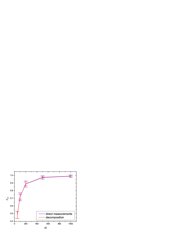
In Figure 8 we show the results for the correlation coefficients on different time scales. The decomposition method gives good results in this case too. The ratio of the standard deviations at $\Delta t=1000$ is close to 3.5, signaling that in order to obtain the same precision, we need roughly one order of magnitude more data points in case of direct measurements than for the decomposition method. Figure 9 shows the extrapolation to the asymptotic value of the correlation, using piecewise Cubic Hermite Interpolation method. The extrapolated curve intercepts the y-axis at the value of 1.002. Applying the extrapolation to the endpoints of the error bars, comparing the direct measurements and the decomposition results, we find a factor of 20 improvement in the precision.

Figure 8: (Color online) Comparison of the directly measured correlation coefficients and the coefficients determined through the decomposition method in case of the persistent random walk, with Weibull sampling. In blue we show the average and the standard deviation of the direct measurements computed over the ensemble of 50 time series pairs. In red we show the average and the standard deviation obtained by the decomposition method, computed over the ensemble of 50 time series pairs.

Figure 9: (Color online) The correlation as a function of $1/\Delta t$ for the persistent random walk, with Weibull sampling. The circles show the correlations determined using the decomposition method, and the (red) curve is determined by using piecewise Cubic Hermite Interpolation method. The extrapolation gives an asymptotic correlation value of 1.002.

4 Demonstration on real data

As discussed in the introduction, an example of correlated asynchronous signals is the case of stock market data. Price changes for different assets on the market appear in an asynchronous manner, however, it is well known that there are important correlations between the price changes. In order to demonstrate our method on real world data, in this Section we show how it can be used to estimate financial correlations.

We took data for Coca-Cola and Pepsi, a pair of stocks with strong correlations from the high frequency Trade and Quote (TAQ) Database of the New York Stock Exchange (NYSE) for the year 2000. We computed the logarithmic returns of stock prices:

$$q^{A}_{\Delta t}(t)=\log\frac{p^{A}(t)}{p^{A}(t-\Delta t)},$$ (12)

where $p^{A}(t)$ stands for the price of stock $A$ at time $t$. The prices were determined using previous tick estimator on the high frequency data, i.e. prices are defined constant between two consecutive trades. What we study is the cross-correlation coefficient between the data of different stocks.

We divided data for the year 2000 into 50 disjoint periods of 5 days (weekly periods) and measured the correlations on these time intervals. This way we handle the separate weeks independently, similar to the case of the generated data: We have $50$ time series pairs and can study both the directly calculated correlation coefficients, both the coefficients obtained through the decomposition method.

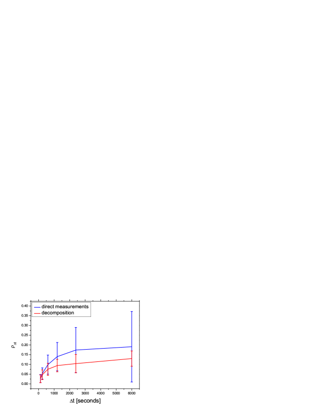
Figure 10 shows the results for the correlation coefficients on different time scales. We can see that the standard deviation of the coefficients obtained through the decomposition are much lower than those of the direct measurements: The ratio of the standard deviations at $\Delta t=6000$ seconds is 4.6 signaling that in order to obtain the same precision, we need roughly 20 times more data points in case of direct measurements than for the decomposition method.

Figure 10: (Color online) Comparison of the directly measured correlation coefficients and the coefficients determined through the decomposition method in case of real world stock market data. The correlations are computed for the stock pair KO/PEP for the year 2000. In blue we show the average and the standard deviation of the direct measurements computed over the ensemble of 50 weekly time series pairs. In red we show the average and the standard deviation obtained by the decomposition method, computed over the ensemble of 50 weekly time series pairs.

5 Summary

In this paper we discussed the problem of estimating the correlation coefficient between two asynchronous signals. While the direct use of high resolution data results in an underestimation of the correlations, coarser binning of the the data leads to larger errors due to loss of data.

We proposed a method, which enables to estimate the asymptotic value of correlations from the high frequency data, without the need of using longer time scales and thus without using worse statistics. The correlations from the high frequency data can be determined very accurately, based on the good statistics. We demonstrated our method on generated data sets, showing that the error of correlations determined by our method is much smaller than the errors of correlations measured directly, using long time windows. Extrapolating to the asymptotic correlation from the determined correlation values leads to a very accurate estimation of the underlying correlation. A very important question in the estimation of the asymptotic correlation value is the determination of the shortest meaningful time scale, $\Delta t_{0}$, on which we measure the decay functions. The asynchronicity of the signals slows down the decrease of the decay functions. In the paper we showed that also in case of non-trivial decay functions the decomposition gives a good estimation of the asymptotic correlation value.

We demonstrated how the method works for real data. When studying weekly cross-correlations of stock returns we showed that the precision of the coefficients obtained through our method is much higher than that of the direct measurements.

Acknowledgements

We thank Zoltán Szatmáry and Zsolt Kajcsos for useful discussions. Support by OTKA K60456 and T049238 is acknowledged.

*

Appendix A The decomposition of correlations

We can write the correlation coefficient from Equation 2 in the following form:

$$\rho_{\Delta t}^{A/B}=\frac{\left\langle\Delta r_{\Delta t}^{A}(t)\Delta r_{\Delta t}^{B}(t)\right\rangle}{\sigma^{A}\sigma^{B}}=$$

$$=\frac{\left\langle r_{\Delta t}^{A}(t)r_{\Delta t}^{B}(t)\right\rangle-\left\langle r_{\Delta t}^{A}(t)\right\rangle\left\langle r_{\Delta t}^{B}(t)\right\rangle}{\sqrt{\left\langle r_{\Delta t}^{A}(t)^{2}\right\rangle-\left\langle r_{\Delta t}^{A}(t)\right\rangle^{2}}\sqrt{\left\langle r_{\Delta t}^{B}(t)^{2}\right\rangle-\left\langle r_{\Delta t}^{B}(t)\right\rangle^{2}}}.$$ (13)

We assume two time scales: $\Delta t$ and $\Delta t_{0}$ where $\Delta t=n\Delta t_{0}$, with $n$ being a positive integer. The change in the measured quantity in the time window $\Delta t$ is the mere sum of changes in shorter, non-overlapping time windows $\Delta t_{0}$:

$$r_{\Delta t}(t)=\sum_{s=1}^{n}r_{\Delta t_{0}}(t-\Delta t+s\Delta t_{0}).$$ (14)

Using this relationship the time average can be written in the following form:

$$\left\langle r_{\Delta t}^{A}(t)r_{\Delta t}^{B}(t)\right\rangle=\frac{1}{T-\Delta t}\sum_{i=\Delta t}^{T}r_{\Delta t}^{A}(i)r_{\Delta t}^{B}(i)=$$

$$=\sum_{s=1}^{n}\sum_{q=1}^{n}\left\langle r_{\Delta t_{0}}^{A}(t-\Delta t+s\Delta t_{0})r_{\Delta t_{0}}^{B}(t-\Delta t+q\Delta t_{0})\right\rangle.$$ (15)

The sum in Eq. A can be written in the following way for stationary signals:

$$\left\langle r_{\Delta t}^{A}(t)r_{\Delta t}^{B}(t)\right\rangle=\sum_{x=-n+1}^{n-1}\left(n-|x|\right)\left\langle r_{\Delta t_{0}}^{A}(t)r_{\Delta t_{0}}^{B}(t+x\Delta t_{0})\right\rangle,$$ (16)

and similarly

$$\left\langle r_{\Delta t}^{A}(t)^{2}\right\rangle=\sum_{x=-n+1}^{n-1}\left(n-|x|\right)\left\langle r_{\Delta t_{0}}^{A}(t)r_{\Delta t_{0}}^{A}(t+x\Delta t_{0})\right\rangle$$

$$\left\langle r_{\Delta t}^{B}(t)^{2}\right\rangle=\sum_{x=-n+1}^{n-1}\left(n-|x|\right)\left\langle r_{\Delta t_{0}}^{B}(t)r_{\Delta t_{0}}^{B}(t+x\Delta t_{0})\right\rangle.$$ (17)

On the other hand, for stationary signals, Equation 14 leads to

$$\left\langle r_{\Delta t}(t)\right\rangle=n\left\langle r_{\Delta t_{0}}(t)\right\rangle.$$ (18)

Combining the above equations we can deduce a relationship between the correlation coefficients measured on two different sampling time scales and we get Equation 2.

References

- [1] G. Hevesy, H. Levi, Action of slow neutrons on rare earth elements, Nature 137 (3457) (1936) 185.
- [2] D. Soete, R. Gijbels, J. Hoste, Neutron Activation Analysis, Wiley Interscience, New York, 1972.
- [3] K. G. McConnell, Vibrational testing: Theory and Practice, John Wiley, New York, 1995.
- [4] T. W. Epps, Comovements in stock prices in the very short run, Journal of the American Statistical Association 74 (1979) 291–298.
- [5] E. W. Montroll, G. H. Weiss, Random walks on lattices, ii, J. Math. Phys. 6 (2) (1965) 167–181.
- [6] H. Scher, M. Lax, Stochastic transport in a disordered solid, i. theory, Physical Review B 7 (1973) 4491–4502.
- [7] E. Scalas, The application of continuous-time random walks in finance and economics, Physica A 362 (2006) 225–239.
- [8] P. Malliavin, M. E. Mancino, Fourier series method for measurement of multivariate volatilities, Finance Stochast. 6 (2002) 49–61.
- [9] R. Renò, A closer look at the epps effect, International Journal of Theoretical and Applied Finance 6 (1) (2003) 87–102.
- [10] O. Precup, G. Iori, A comparison of high-frequency cross-correlation measures, Physica A 344 (1-2) (2004) 252–256.
- [11] T. Hayashi, N. Yoshida, On covariance estimation of non-synchronously observed diffusion processes, Bernoulli 11 (2) (2005) 359–379.
- [12] V. Voev, A. Lunde, Integrated covariance estimation using high-frequency data in the presence of noise, Journal of Financial Econometrics 5 (1) (2006) 68–104.
-
[13]
A. Palandri, Consistent realized covariance for asynchronous observations
contaminated by market microstructure noise.
URL http://www.econ.ku.dk/Events_News/Zeuthen/2006/Workshop_06
/Papers/Palandri_RealCorr2.pdf -
[14]
B. Tóth, J. Kertész, The epps effect revisited.
URL http://arxiv.org/pdf/0704.1099 - [15] R. Furth, Ann. Phys. (Leipzig) 43 (1917) 177.
- [16] G. H. Weiss, Aspects and Applications of the Random Walk, North-Holland, Amsterdam, 1994.