Density of states of disordered graphene

Abstract

We calculate the average single particle density of states in graphene with disorder due to impurity potentials. For unscreened short-ranged impurities, we use the non-self-consistent and self-consistent Born and $T$-matrix approximations to obtain the self-energy. Among these, only the self-consistent $T$-matrix approximation gives a non-zero density of states at the Dirac point. The density of states at the Dirac point is non-analytic in the impurity potential. For screened short-ranged and charged long-range impurity potentials, the density of states near the Dirac point typically increases in the presence of impurities, compared to that of the pure system.

I introduction

The recent experimental realization of a single layer of carbon atoms arranged in a honey-comb lattice has prompted much excitement and activity in both the experimental and theoretical physics communities review ; neto . Carriers in graphene (both electrons and holes) have a linear bare kinetic energy dispersion spectra around the $K$ and $K^{\prime}$ points (the “Dirac points”) of the Brillouin zone. The ability of experimentalists to tune the chemical potential to lie above or below the Dirac point energy (by application of voltages to gates in close proximity to the graphene sheets) allows the carriers to be changed from electrons to holes in the same sample. This sets graphene apart from other two dimensional (2D) carrier systems that have a parabolic dispersion relation, and typically have only one set of carriers, i.e. either electrons or holes. Another unique electronic property, the absence of back-scattering, has led to the speculation that carrier mobilities of 2D graphene monolayers (certainly at room temperature, but also at low temperature) could be made to be much higher than any other field-effect type device, suggesting great potential both for graphene to be the successor to Si-MOSFET (metal-oxide-semicondcutor field effect transistor) devices and for the discovery of new phenomena that normally accompanies any significant increase in carrier mobility Hwang et al. (2007); Ando (2006); bolotin ; geim . It is therefore of considerable fundamental and technological interest to understand the electronic properties of graphene neto .

Graphene samples that are currently being fabricated are far from pure, based on the relatively low electronic mobilities compared to epitaxially grown modulation-doped two-dimensional electron gases (2DEGs) such as GaAs-AlGaAs quantum wells. It is therefore important to understand the effects of disorder on the properties of graphene. Disorder manifests itself in the finite lifetimes of electronic eigenstates of the pure system. In the presence of scattering from an impurity potential that is not diagonal in the these eigenstates, the lifetime scattering rate of the eigenstate, $\gamma$, is non-zero and can be measured experimentally by fitting the line-shape of the low-field Shubnikov-de Haas (SdH) oscillations. Harrang et al. (1985); Lukyanchuk and Kopelevich (2006) The effect of disorder scattering on the SdH line shape is equivalent to increasing the sample temperature and one can therefore measure this Dingle temperature ($T_{D}$) and relate it to the single-particle lifetime through $\hbar\gamma=2\pi k_{B}T_{D}$. To avoid potential confusion, we mention that the lifetime damping rate $\gamma$ discussed in this paper is not equal to the transport scattering rate which governs the electrical conductivity. The lifetime damping rate is the measure of the rate at which particles scatters out of an eigenstate, whereas the transport scattering rate is a measure of the rate of current decay due to scattering out of an eigenstate. In normal 2DEGs, the transport scattering time can be much larger than the impurity induced lifetime $\hbar/2\gamma$, particularly in high mobility modulation doped 2D systems where the charged impurities are placed very far from the 2DEGHarrang et al. (1985); Das Sarma and Stern (1985). Recently, the issue of transport scattering time versus impurity scattering lifetime in graphene has been discussed.hwang_single

The single-particle level broadening due to the impurity potential changes many of the physical properties of the system including the electronic density of states.Das Sarma and Vinter (1981); Ando et al. (1982) The electronic density of states is an important property which directly affects many experimentally measurable quantities such as the electrical conductivity, thermoelectric effects, and differential conductivity in tunneling experiments between graphene and scanning-tunneling microscope tips or other electron gases. Changes in the density of states also modify the electron screening,Ando (1982) which is an important factor in the determination of various properties of graphene. It is therefore imperative to take into account the effects of disorder on the density of states, particularly since disorder is quite strong in currently available graphene samples.

In the present work, we present calculations of the average density of states of disordered graphene. This problem has been investigated using various models and techniques, both analytical and numerical.hu1984 ; fradkin ; peres2006 ; pereira ; skrypnyk ; dora2008 ; wu2008 ; lherbier2008 We take into account scattering effects from long-range and short range impurity potentials. We consider both unscreened and screened short-ranged and screened charged impurities, using the Born approximation. In addition, for unscreened short-ranged (USR) impurities, we go beyond the Born approximation and include self-consistent effects.

There is another class of disorder in graphene called “off-diagonal” or “random gauge potential” disorder, in which the hopping matrix elements of the electrons in the underlying honeycomb lattice are random. In this paper we do not consider in this type of disorder, which can result from height fluctuations (ripples) in the graphene sheet and lead to qualitatively different results from the ones presented in this paper.hu1984 ; dora2008 ; morita1997 ; guinea2008

The rest of the paper is organized as follows: In Sec. II, we describe the approximation schemes that we use. Secs. III and IV deal with unscreened short range impurities and screened short-range/charged impurities, respectively. In Sec. V, we compare our results to those from other workers, and we conclude in Sec. VI.

II Approximations for the self-energy

The single-particle density of states for a translationally invariant 2DEG is given byrickmah

$$D(E) =-\frac{g}{\pi}\sum_{\lambda}\int\frac{d\bm{k}}{(2\pi)^{2}}\ {{\rm Im}}[G_{\lambda}(\bm{k},E)]$$ (1)

where $g$ is the degeneracy factor (for graphene $g=4$ due to valley and spin degeneracies) $\lambda$ is the band index, $G$ is the retarded Green’s function, and the $\bm{k}$-integration is over a single valley, which we assume to be a circle of radius $|\bm{k}|=k_{c}$. $G$ expressed in terms of the retarded self-energy $\Sigma_{\lambda}(\bm{k},\omega)$ is

$$G_{\lambda}(\bm{k},E)=[E-E_{\bm{k},\lambda}-\Sigma_{\lambda}(\bm{k},E)+i\eta]^{-1}.$$ (2)

where $E_{\bm{k},\lambda}$ is the bare band energy of the state $|\bm{k}\lambda\rangle$ and $\eta$ is an infinitesimally small positive number. (In this paper, the Green’s functions and self-energies are all assumed to be retarded.) Eqs. (1) and (2) show that if $E_{\bm{k},\lambda}$ and $\Sigma_{\lambda}(\bm{k},E)$ are known, the density of states can be obtained in principle from

$$D(E)=\frac{g}{\pi}\sum_{\lambda}\int\frac{d\bm{k}}{(2\pi)^{2}}\ \frac{-{{\rm Im}}[\Sigma_{\lambda}(\bm{k},E)]+\eta}{(E-E_{\bm{k},\lambda}-{\rm Re}[\Sigma_{\lambda}(\bm{k},E)])^{2}+({\rm Im}[\Sigma_{\lambda}(\bm{k},E)]-\eta)^{2}}.$$ (3)

For pure graphene systems, $\Sigma(\bm{k},E)=0$ (excluding electron–electron and electron–phonon interactions, which are not considered here), and hence ${\rm Im}[G_{\lambda}(\bm{k},E)]=-\pi\delta(E-E_{\bm{k}\lambda})$. Close to the Dirac points (which we choose to the the zero of energy), the dispersion for graphene is (we use $\hbar=1$ throughout this paper)

$$E_{\bm{k},\lambda}=\lambda v_{F}k,$$ (4)

where $\lambda=+1$ and $-1$ for the conduction and valence bands, respectively, $k=|\bm{k}|$ is the wavevector with respect to the Dirac point, and $v_{F}$ is the Fermi velocity of graphene. Performing the $\bm{k}$-integration in Eq. (1) for the pure graphene case gives

$$D_{0}(E)=\frac{g}{2\pi}\frac{|E|}{v_{F}^{2}}\,\theta(|E|-E_{c}),$$ (5)

where $E_{c}=v_{F}k_{c}$ is the band energy cut-off.

The average density of states for a disordered 2DEG can be obtained by averaging the Green’s function over impurity configurations. The averaging procedure gives a non-zero $\Sigma$ which, in general, cannot be evaluated exactly. Various approximation schemes for $\Sigma$ have therefore been developed, four of which are described below.

Figure 1: Feynman diagrams for the (a) Born and (b) $T$-matrix approximations for the self-energy. The “x”, dotted line and line with arrow signify the impurity, impurity potential, and Green’s function, respectively. The Green’s functions are either bare or self-consistent.

Born Approximation — In the Born approximation, the self-energy is given by the Feynman diagram shown in Fig. 1(a)rickmah , and the expression for the self-energy is

$$\Sigma_{B,\lambda}(\bm{k},E)=n_{i}\int\frac{d\bm{k}^{\prime}}{(2\pi)^{2}}\ |U(\bm{k}-\bm{k}^{\prime})|^{2}\;$$

$$\times\sum_{\lambda^{\prime}}G_{0,\lambda^{\prime}}(\bm{k}^{\prime},E)\;F_{\lambda\lambda^{\prime}}(\bm{k},\bm{k}^{\prime})$$ (6)

where $n_{i}$ is the impurity density, $U(\bm{q})$ is the Fourier transform of the impurity potential, $G_{0}$ is the bare Green’s function and $F_{\lambda\lambda^{\prime}}(\bm{k},\bm{k}^{\prime})$ is square of the the overlap function between the part of the wavefunctions of $|\bm{k}\lambda\rangle$ and $|\bm{k}^{\prime}\lambda^{\prime}\rangle$ that are periodic with the lattice (here $\lambda,\lambda^{\prime}$ are band indices). For graphene states near the Dirac point,

$$F_{\lambda\lambda^{\prime}}(\bm{k},\bm{k}^{\prime})=\frac{1}{2}(1+\lambda\lambda^{\prime}\cos\theta_{\bm{k}\bm{k}^{\prime}}),$$ (7)

where $\theta_{\bm{k}\bm{k}^{\prime}}$ is the angle between $\bm{k}$ and $\bm{k}^{\prime}$.

Self-Consistent Born Approximation — The Feynman diagram for this self-energy is the same as Fig. 1(a), except that the bare Green’s function is replaced by the full one. Consequently, the expression for $\Sigma_{\rm SB}$ is the same as in Eq. (6), except with $G_{0}$ replaced by $G$.

$T$-matrix Approximation — The $T$-matrix approximation is equivalent to the summation of Feynman diagrams shown Fig. 1(b). The expression for $\Sigma_{T}$ is the same as in Eq. (6), except with $U$ replaced by $T$, the $T$-matrix for an individual impurity.

Self-consistent $T$-matrix Approximation — The Feynman diagram for this approximation is the same as in the $T$-matrix approximation, except that the bare Green’s functions are replaced by full ones. The expression for $\Sigma_{{\rm S}T}$ is the same as in Eq. (6), except with $U$ replaced by $T$, and $G_{0}$ replaced by $G$.

When the potentials for the impurities are not all identical (for example, in the case where there is a distribution of distances of charged impurities from the graphene sheet), one averages $|U(\bm{k}-\bm{k}^{\prime})|^{2}$ or $|T(\bm{k}-\bm{k}^{\prime})|^{2}$ over the impurities.

III Unscreened short-ranged (USR) disorder

In the present context, short-ranged impurities are impurities which result from localized structural defects in the honeycomb lattice, which are roughly on the length scale of the lattice constant. In this case, it is acceptable to approximate $U(\bm{q})=U_{0}$, a real constant, for intravalley scattering processes. In this paper, we ignore the intervalley processes. (However, we note that if the matrix element joining intervalley states is constant, inclusion of intervalley scattering in our calculations is not difficult.) This simplification allows us to obtain some analytic expressions for the self-energies in the approximation schemes mentioned above.

III.1 Self-energy for USR disorder

For USR disorder, the four approximation schemes we use give self-energies that are independent of $\lambda$ and $k$.

III.1.1 Born approximation

The self-energy for graphene with USR scatterers in the Born approximation, using $U(\bm{q})=U_{0}$, Eqs. (4) and (7) in Eq. (6), is

$$\Sigma^{\rm(usr)}_{B}(E) =\tilde{\gamma}_{B}H_{0}(E+i\eta);$$ (8a)

$$\tilde{\gamma}_{B} =\frac{n_{i}U_{0}^{2}}{2v_{F}^{2}};$$ (8b)

$$H_{0}(\zeta) =2v_{F}^{2}\sum_{\lambda^{\prime}}\int\frac{d\bm{k}^{\prime}}{(2\pi)^{2}}\ G_{0,\lambda^{\prime}}(\bm{k}^{\prime},\zeta)F_{\lambda\lambda^{\prime}}(\bm{k},\bm{k}^{\prime})$$

$$=\int_{0}^{E_{c}}\frac{dE^{\prime}}{2\pi}\left(\frac{E^{\prime}}{\zeta-E^{\prime}}+\frac{E^{\prime}}{\zeta+E^{\prime}}\right)$$

$$=-\frac{\zeta}{2\pi}\ln\left(1-\frac{E_{c}^{2}}{\zeta^{2}}\right).$$ (8c)

As a function of complex $\zeta$, $H_{0}(\zeta)$ is real and positive (negative) along the real axis from $E_{c}$ to $\infty$ ($-E_{c}$ to $-\infty$). Furthermore, it has a branch cut in on the real axis of $\zeta$ in between $-E_{c}$ and $E_{c}$, so that for $-E_{c}<E\ \mbox{(real)}<E_{c}$,

$$H_{0}(E\pm i\eta)=-(2\pi)^{-1}\left(E\ln\left|\frac{E_{c}^{2}}{E^{2}}-1\right|\pm i\pi|E|\right).$$ (9)

Fig. 2 shows $H_{0}(E+i\eta)$.

For real $E$ and $|E|\ll E_{c}$,

$$\Sigma^{\rm(usr)}_{B}(E)\approx-\frac{\tilde{\gamma}_{B}}{2}\left[\frac{2E}{\pi}\,\ln\left|\frac{E}{E_{c}}\right|+i|E|\right].$$ (10)

The Born approximation damping rate for state $|\bm{k}\lambda\rangle$ is $\gamma_{B}(k)=-2{\rm Im}[\Sigma_{B}^{\rm(usr)}(E_{\bm{k},\lambda})]=\tilde{\gamma}_{B}\,v_{F}k$.

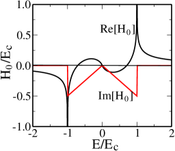
Figure 2: Real and imaginary parts of $H_{0}(E+i\eta)=\Sigma_{B}^{\rm(usr)}(E)/\tilde{\gamma}_{B}$ [see Eq. (9)], where $\Sigma_{B}^{\rm(usr)}(E)$ is the self-energy for USR impurities in the Born approximation.

III.1.2 Self-consistent Born approximation

The self-energy $\Sigma_{\rm SB}^{\rm(usr)}$ for unscreened short-ranged scatterers in the self-consistent Born approximation is given by the self-consistent equation

$$\Sigma_{\rm SB}^{\rm(usr)}(E) =\tilde{\gamma}_{B}\,H_{\rm SB}(E+i\eta);$$ (11a)

$$H_{\rm SB}(\zeta) =-\frac{1}{2\pi}\left[\zeta-\Sigma_{\rm SB}^{\rm(usr)}(\zeta)\right]\ln\left[1-\frac{E_{c}^{2}}{[\zeta-\Sigma_{\rm SB}^{\rm(usr)}(\zeta)]^{2}}\right]$$

$$=H_{0}\left[\zeta-\Sigma_{\rm SB}^{\rm(usr)}(\zeta)\right],$$ (11b)

This shows that if $|\Sigma_{\rm SB}^{\rm(usr)}(E)|\ll|E|$, then $\Sigma_{SB}^{\rm(usr)}(E)\approx\Sigma_{B}^{\rm(usr)}(E)$ (except possibly around $E=\pm E_{c}$, which is usually not experimentally relevant).

III.1.3 $T$-matrix approximation

In general the impurity averaged $T$-matrix for a potential $U(\bm{q})$ is

$$T_{\bm{k}_{0}\lambda_{0},\bm{k}\lambda}(E)=n_{i}\sum_{n=1}^{\infty}\left[\left(\prod_{i=1}^{n}\sum_{\lambda_{i}=\pm 1}\int\frac{d\bm{k}_{i}}{(2\pi)^{2}}U(\bm{k}_{i-1}-\bm{k}_{i})\,G_{0,\lambda_{i}}(\bm{k}_{i},E)\,F_{\lambda_{i-1},\lambda_{i}}(\bm{k}_{i-1},\bm{k}_{i})\right)U(\bm{k}_{i}-\bm{k})\,F_{\lambda_{n},\lambda}(\bm{k}_{n},\bm{k})\right].$$ (12)

In this approximation, the self energy is

$$\Sigma_{T,\lambda}(\bm{k},E)=T_{\bm{k}\lambda,\bm{k}\lambda}(E).$$ (13)

If $U(\bm{q})=U_{0}$, a constant, the term in the square parentheses in Eq. (12) is $U_{0}^{n+1}H_{0}^{n}(E+i\eta)/(2v_{F}^{2})^{n}$. The sum then gives

$$\Sigma^{\rm(usr)}_{T}(E)=\frac{\tilde{\gamma}_{B}H_{0}(E+i\eta)}{\displaystyle 1-\frac{U_{0}}{2v_{F}^{2}}H_{0}(E+i\eta)}.$$ (14)

III.1.4 Self-consistent $T$-matrix approximation

As in self-consistent Born approximation, the $H_{0}(E)$ in Eq. (14) is replaced by the self-consistent $H_{{\rm S}T}(E)$, giving

$$\Sigma^{\rm(usr)}_{\mathrm{S}T}(E) =\frac{\tilde{\gamma}_{B}H_{{\rm S}T}(E+i\eta)}{\displaystyle 1-\frac{U_{0}}{2v_{F}^{2}}H_{{\rm S}T}(E+i\eta)};$$ (15a)

$$H_{{\rm S}T}(\zeta) =H_{0}\left(\zeta-\Sigma_{{\rm S}T}^{\rm(usr)}(\zeta)\right).$$ (15b)

As in the self-consistent Born approximation, this shows that if $|\Sigma_{{\rm S}T}^{\rm(usr)}(E)|\ll|E|$, then $\Sigma_{{\rm S}T}^{\rm(usr)}(E)\approx\Sigma_{T}^{\rm(usr)}(E)$ (except possibly around $E=\pm E_{c}$).

III.2 Density of states for $\bm{k}$-independent $\Sigma$

When the self-energy is $\bm{k}$- and $\lambda$-independent, the density of states for graphene can be calculated analytically from Eq. (3). The result is

$$D(E) =\frac{g_{s}g_{v}}{2\pi^{2}v_{F}^{2}}\Biggl{\{}\frac{\Gamma}{2}\ln\left(\frac{(E_{c}^{2}+\Omega^{2}+\Gamma^{2})^{2}-4E_{c}^{2}\Omega^{2}}{(\Omega^{2}+\Gamma^{2})^{2}}\right)+\Omega\left[\tan^{-1}\left(\frac{E_{c}-\Omega}{\Gamma}\right)-\tan^{-1}\left(\frac{E_{c}+\Omega}{\Gamma}\right)+2\tan^{-1}\left(\frac{\Omega}{\Gamma}\right)\right]\Biggr{\}},$$ (16)

where $\Gamma(E)=-{\rm Im}[\Sigma(E)]$ and $\Omega(E)=E-{\rm Re}\![\Sigma(E)]$.

III.3 Density of states at the Dirac point

There has been considerable interest in the minimum DC electrical conductivity of disordered graphene as the Fermi energy moves through the Dirac point.Novoselov et al. (2005); tan2007 There is still no consensus on whether the minimum conductivity is a universal value or not. Since the electrical conductivity is directly proportional to the density of states at the Fermi energy, it is important to be able to determine the density of states at the Dirac point of disordered graphene. Because the minimum conductivity is non-zero as the Fermi energy passes through the Dirac point, the density of states should be nonzero.

Eq. (3) shows that if $\Sigma(E)\rightarrow 0$ when $E\rightarrow 0$, then the density of states at the Dirac point $D(0)=0$. (Note that we have not included the term that is first order in the impurity potential in our self-energy. Since this first-order term merely rigidly shifts the band by an amount $n_{i}U_{0}$, ignoring this term is equivalent to shifting the zero of the energy by $-n_{i}U_{0}$, and hence the Dirac point is still at $E=0$.) A non-zero density of states at the Dirac point depends on a non-zero ${\rm Im}[\Sigma(E=0)]$. Since $H_{0}(E\rightarrow 0)=0$, it is clear from Eqs. (8a) and (14) that the Born and $T$-matrix approximations give zero density of states at the Dirac point.

For the self-consistent Born approximation, Eq. (11b) can be rewritten as

$$\Sigma_{\rm SB,\lambda}^{\rm(usr)}(E) =E\left[1+\frac{2\pi}{\tilde{\gamma}_{B}\ln\left(1-\frac{E_{c}^{2}}{(E-\Sigma_{\rm SB,\lambda}^{\rm(usr)}(E))^{2}}\right)}\right]^{-1},$$ (17)

which shows that $\Sigma_{\rm SB,\lambda}^{\rm(usr)}(E\rightarrow 0)=0$, and therefore the self-consistent Born approximation also gives $D(0)=0$.

In the case of the self-consistent $T$-matrix approximation, re-writing Eq (15a) as

$$\Sigma_{\mathrm{S}T}^{\rm(usr)}(E)+n_{i}U_{0}=\frac{n_{i}U_{0}}{1-H_{0}(E-\Sigma_{\mathrm{S}T}^{\rm(usr)}(E))U_{0}/(2v_{F}^{2})},$$ (18)

setting $E=0$, using Eq. (8c) and taking the imaginary parts of both sides of this equation gives

$${\rm Im}[\Sigma(0)]\equiv\Gamma(0) ={\rm Im}\left[\frac{n_{i}U_{0}}{\displaystyle 1-i\frac{U_{0}\Gamma(0)}{2v_{F}^{2}}\ln\left(1+\frac{E_{c}^{2}}{\Gamma(0)^{2}}\right)}\right].$$ (19)

In the weak scattering limit, when $\tilde{\gamma}_{B}\ll 1$, the imaginary term in the denominator of Eq. (19) is much less than one (we check for self-consistency later), and this gives

$$\Gamma_{w}(0) \approx{\rm Im}\left[i\frac{n_{i}\Gamma_{w}(0)U_{0}^{2}}{v_{F}^{2}}\ln\left(\frac{E_{c}}{\Gamma_{w}(0)}\right)\right]=2\tilde{\gamma}_{B}\Gamma_{w}(0)\ln\left(\frac{E_{c}}{\Gamma_{w}(0)}\right),$$ (20)

which implies that

$$\Gamma_{w}(0)=E_{c}\exp\left(-\frac{1}{2\tilde{\gamma}_{B}}\right).$$ (21)

Note that the result is non-analytic in $U_{0}$. Inserting Eq. (21) into the imaginary part of the denominator of Eq. (19) (which we had assumed to be much smaller than 1 in magnitude) gives the self-consistent criterion $\exp(-1/2\tilde{\gamma}_{B})\ll n_{i}U_{0}/E_{c}$ for the validity of Eq. (21). Substituting this into Eq. (16) gives an average density of states at the Dirac point for weak scattering of approximately

$$\rho_{w}(0)=\frac{g_{s}g_{v}E_{c}}{\pi^{2}n_{i}U_{0}^{2}}\exp\left(-\frac{1}{2\tilde{\gamma}_{B}}\right).$$ (22)

Similar results to Eq. (22) have been reportedfradkin ; dora2008 ; ostrovsky2006 in studies of disordered systems of fermions with linear dispersions using other methods.

We mention that our calculation of the graphene density of states at the Dirac point should only be considered as demonstrative since electron-electron interaction effects are crucial dassarma_ee at the Dirac point, and the undoped graphene system is not a simple Fermi liquid at the Dirac point.

IV Screened short-ranged and charged impurities

Free carriers will move to screen a bare impurity potential $V_{\rm ei}(q)$, resulting in a screened interaction $U(q)=V_{\rm ei}(q)/\varepsilon(q)$, where $\varepsilon(q)$ is the static dielectric function. The $\varepsilon(q)$ results in an $q$-dependent effective electron-impurity potential $U$, even in the case of short-ranged ($q$-independent) bare impurity potentials. This makes the calculations much more involved than in the USR case. Therefore, in this paper, we limit our investigation of $q$-dependent screened potentials to the level of the Born approximation.

For the dielectric function $\varepsilon(q)$, we use the random phase approximation (RPA) for dielectric function appropriate for graphene, given by $\varepsilon(q)=1-V_{c}(q)\Pi_{0}(q)$ where $V_{c}(q)=2\pi e^{2}/(\kappa q)$ is the two-dimensional Fourier transform of the Coulomb potential ($\kappa$ is the dielectric constant of the surrounding material), and $\Pi_{0}(q)$ is the static irreducible RPA polarizability for graphene.Hwang and S. Das Sarma (2007) We use $V_{\rm ei}(q)=V_{c}(q)$ for charged impurities, and $V_{\rm ei}(q)=U_{0}$, a constant, for short-range point defect scatterers.

We first look at the density of states at the Fermi surface; i.e., at energy $E=\lambda k_{F}v_{F}$. To obtain this, we calculate the single-particle lifetime damping rate $\gamma$ in the Born approximation, which is given by

$$\gamma_{\lambda}(k) = -2{\rm Im}[\Sigma_{\lambda}(k,E_{k\lambda})]$$ (23)

$$= \frac{n_{i}}{2\pi}\frac{k}{v_{F}}\int_{0}^{\pi}d\theta\ \frac{\langle\left|{V_{ei}(q)}\right|^{2}\rangle}{\varepsilon(q)^{2}}(1+\cos\theta),$$

where $q=2k\sin(\theta/2)$. Then, assuming that ${\rm Im}[\Sigma_{\lambda}(k,E)]$ is relatively constant for $k$ close to $k_{F}$, we substitute $\frac{1}{2}\gamma_{\lambda}(k_{F})$ for $-{\rm Im}[\Sigma_{\lambda}(\bm{k},E_{F})]$ into Eq. (3), which gives Eq. (16) with $\Gamma=\frac{1}{2}\gamma_{\lambda}(k_{F})$.

We assume that the charged or neutral impurities are distributed completely at random on the surface of the insulating substrate on which the graphene layer lies, the areal density for the charged and neutral impurities is $n_{ic}$ and $n_{i\delta}$, respectively, and the density of carriers in the graphene layer is $n=k_{F}^{2}/\pi$, where $k_{F}$ is the Fermi wavevector relative to the Dirac point. (This relationship between $n$ and $k_{F}$ takes into account the spin and valley degeneracy $g_{s}=2$ and $g_{v}=2$.) We use the RPA screening function at $T=0$,Hwang and S. Das Sarma (2007) to obtain the effective impurity potential. The key dimensionless parameter that quantifies the screening strength is $r_{s}=e^{2}/(\kappa v_{F})$, which is corresponding to the interaction strength parameter of a normal 2D system (i.e. the ratio of potential energy to kinetic energy). The Born approximation lifetime damping rates for screened charged-impurities $\gamma_{c}$ and $\delta$-correlated neutral impurities $\gamma_{\delta}$ at $k_{F}$ are

$$\gamma_{c}(k_{F}) =\frac{n_{ic}E_{F}}{4n}\;I_{c}(2r_{s});$$ (24a)

$$\gamma_{\delta}(k_{F}) =\frac{2E_{F}\tilde{\gamma}_{B}}{\pi}\;I_{\delta}(2r_{s}).$$ (24b)

In these equations,

$$I_{c}(x) =x-\frac{\pi x^{2}}{2}+x^{3}\,f(x);$$ (25a)

$$I_{\delta}(x) =\frac{\pi}{4}+3x\left(1-\frac{\pi x}{2}\right)+x(3x^{2}-2)f(x),$$ (25b)

where

$$f(x) =\left\{\begin{array}[]{cl}\frac{1}{\sqrt{1-x^{2}}}\ln\left[\frac{1+\sqrt{1-x^{2}}}{x}\right]&\mbox{for $x<1$};\\ 1&\mbox{for $x=1$};\\ \frac{1}{\sqrt{x^{2}-1}}\cos^{-1}\frac{1}{x}&\mbox{for $x>1$}.\end{array}\right.$$ (29)

In Fig. 3 we show the calculated damping rates scaled by $|E_{F}|/=k_{F}v_{F}$ as a function the interaction parameter $r_{s}$. For $r_{s}\ll 1$ we have ${\gamma_{c}}/{E_{F}}\approx{n_{ic}r_{s}}/{2n}$ and ${\gamma_{\delta}}/{E_{F}}\approx\tilde{\gamma}_{B}/2$. For $r_{s}\gg 1$ we have ${\gamma_{c}}/{E_{F}}\approx\pi n_{ic}/{16n}$ and ${\gamma_{\delta}}/{E_{F}}\approx\tilde{\gamma}_{B}/(2\pi r_{s})$. Thus, for small (large) $r_{s}$ the damping rate due to the short-ranged impurity dominates over that due to the long-ranged charged impurity. On the other hand, since $\gamma_{c}(k_{F})\propto k_{F}^{-1}\propto n^{-\frac{1}{2}}$ and $\gamma_{\delta}(k_{F})\propto k_{F}\propto n^{\frac{1}{2}}$ [Eq. (24)], in the low (high) carrier density limit the lifetime damping of single particle states at the Fermi surface is dominated by charged impurity (short-ranged impurity) scattering. The crossover takes place around a density

$$n_{\rm cross}=\frac{n_{ic}}{n_{i\delta}}\frac{\pi v_{F}^{2}}{4U_{0}^{2}}\frac{I_{c}(2r_{s})}{I_{\delta}(2r_{s})}.$$ (30)

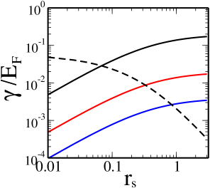
Figure 3: Calculated damping rates scaled by Fermi energy $\gamma/E_{F}$ as a function of $r_{s}$. Graphene on a SiO₂ (air) substrate has an $r_{s}\approx 0.7$ (2). Solid lines indicate damping rates ($\gamma_{c}$) due to charged impurities with an impurity density $n_{ic}=10^{11}{\rm cm}^{-2}$ for different electron densities $n=1$, 10, 50$\times 10^{11}$ cm^-2 (from top to bottom), respectively. Dashed line indicate the damping rate ($\gamma_{\delta}$) due to short-ranged impurity with impurity density $n_{i\delta}=10^{11}$ cm^-2 and potential strength $U_{0}=$1 KeV Ų, which correspond to $\tilde{\gamma}_{B}=0.11$. Note $\gamma_{\delta}/E_{F}$ is independent on the electron density.

Using $\Gamma=\gamma_{\lambda}(k_{F})/2$ in Eq. (16) gives (assuming $E_{F}$, $\Gamma\ll E_{c}$)

$$D(E_{F})\approx D_{0}(E_{F})\left[\frac{1}{2}+\frac{1}{\pi}\tan^{-1}\left(\frac{|E_{F}|}{\Gamma}\right)\right.$$

$$\left.+\frac{\Gamma}{2\pi|E_{F}|}\ln\left(\frac{E_{c}^{2}}{E_{F}^{2}+\Gamma^{2}}\right)\right].$$ (31)

For $\Gamma/|E_{F}|\ll 1$, this gives

$$D(E_{F})\approx D_{0}(E_{F})\left\{1+\frac{1}{\pi}\frac{\Gamma}{|E_{F}|}\left[\ln\left(\frac{E_{c}}{|E_{F}|}\right)-1\right]\right\},$$ (32)

and for $|E_{F}|/\Gamma\ll 1$

$$D(E_{F})\approx D_{0}(E_{F})\left[\frac{1}{2}+\frac{|E_{F}|}{\pi\Gamma}\right]+\frac{g_{s}g_{v}}{2\pi^{2}}\frac{\Gamma}{v_{F}^{2}}\ln\left(\frac{E_{c}}{\Gamma}\right).$$ (33)

We can apply Eq. (32) for short-ranged impurity scattering and for charged impurity scattering in high carrier density limits, and Eq. (33) for charged impurity scattering in low density limits. Taking the limit $|E_{F}|\rightarrow 0$ in Eq. (33), it appears that for the case of screened Charged impurities, we obtain a finite density of states at the Dirac point with the Born approximation (since $\Gamma\propto\gamma_{c}(k_{F})\propto k_{F}^{-1}$). However, recall that in deriving Eqs. (32) and (33), we have assumed that $\Sigma(k,E_{F})$ is constant with respect to $k$, which is not necessarily the case at the Dirac point.

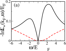
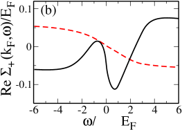
Figure 4: (a) Imaginary and (b) real parts of self energy of a disordered graphene at $k=k_{F}$ for screened Coulomb scattering potential (solid lines) and for screened neutral short-ranged scattering potential (dashed lines).

In general, the damping rate (or the imaginary part of the self energy) is a function of energy and wave vector rather than a constant. From Eq. (6), we calculated the self-energy of disordered graphene. Fig. 4 we show the self-energy of a conduction band electron ($\lambda=+1$) for both screened Coulomb scattering potential and screened neutral short-ranged potential. For Coulomb scatterers we use the impurity density $n_{ic}=10^{12}$ cm^-2, and for neutral short-ranged scatterers the impurity density $n_{i\delta}=10^{11}$ cm^-2 and potential strength $U_{0}=$1 KeV Ų. The self-energies in the valence band ($\lambda=-1$) are related to the self-energy in the conduction band by $\rm{Re}\Sigma_{+}(k,\omega)=-\rm{Re}\Sigma_{-}(k,-\omega)$ and $\rm{Im}\Sigma_{+}(k,\omega)=\rm{Im}\Sigma_{-}(k,-\omega)$. As $\omega\rightarrow 0$, $-{\rm Im}\Sigma_{\lambda}(k_{F},\omega)\rightarrow|\omega|$, and ${\rm Re}\Sigma_{\lambda}(k_{F},\omega)\rightarrow\omega\ln|\omega|$ for both scattering potentials. However, for large value of $|\omega|$ the asymptotic behaviors are different, that is, as $|\omega|\rightarrow\infty$ $-{\rm Im}\Sigma(k_{F},\omega)\propto|\omega|^{-1}$ for Coulomb scattering potential and $-{\rm Im}\Sigma(k_{F},\omega)\propto|\omega|$ for short-ranged potential. Note that by using only the (non-self-consistent) Born approximation in this section, we assume weak scattering and ignoring multiple-scattering events in calculated $\Sigma(k,\omega)$. Therefore, the results are unreliable in the strong disorder limit (i.e., when $\Sigma(k,\omega)$ is modified significantly from its lowest-order form).

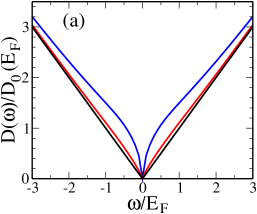
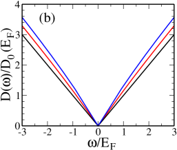
Figure 5: The density of states in the presence of impurity (a) for screened Coulomb potential and (b) for screened short-ranged potential. In (a) we use the charged impurity densities $n_{ic}=0$, 1, $5\times 10^{12}$ cm^-2 (from bottom to top), and in (b) the short-ranged impurity density $n_{id}=0$, 0.5, $1\times 10^{12}$ cm^-2 (from bottom to top) and potential strength $U_{0}=$1 KeV Ų.

In Fig. 5 the density of states in the presence of impurity is shown for different impurity densities. In Fig. 5(a) we show the density of states for Coulomb impurity potential with impurity densities, $n_{ic}=0$, $10^{12}$ cm^-2, $5\times 10^{12}$ cm^-2 (from bottom to top), and in Fig. 5(b) we show the density of states for neutral short-ranged impurity potential with densities, $n_{id}=0$, $5\times 10^{11}$ cm^-2, $10^{12}$ cm^-2 (from bottom to top) and potential strength $U_{0}=$1 KeV Ų. The calculated density of states is normalized by $D_{0}(E_{F})=(g_{s}g_{v}/2\pi)E_{F}/\gamma^{2}$. The density of states is enhanced near Dirac point ($E=0$), but as $|E|\rightarrow 0$ it goes zero as $D(E)\rightarrow|E|\ln|E|$ for both types of screened impurity scattering. Based on the results of Section III, we expect that this result is an artifact of the Born approximation, and that the density of states should in fact be non-zero. The enhancement of the density of states can be explained as follows. In normal 2D system with finite disorder the band edge $E_{{\rm edge},0}$ of the pure conduction (valence) band is shifted to $E_{\rm edge,imp}<0$ ($>0$) and a band tail forms below (above) the band edge of a pure system. Thus, the density of states in the presence of impurities is reduced for $E>0$ ($E<0$) because the states have been shifted by the impurity potential into the band tail. However, for graphene since the conduction band and the valence band meet at the Dirac point the band tail (or shift of band edge) cannot be formed, which gives rise to enhancement of density of states near Dirac point.

Before concluding we point out that our perturbative calculation of the graphene density of states assumes that the system remains homogeneous in the presence of impurities. It is, however, believed Hwang et al. (2007); rossi that graphene carriers develop strong density inhomogeneous (i.e. electron-hole puddle) at low enough carrier densities in the presence of charged impurities due to the breakdown of linear scattering. In such an inhomogeneous low-density regime close to the Dirac point, our homogeneous perturbative calculation does not apply.

V Comparisons to other works

In this section, we compare and contrast our model of disorder and results to other works in the field.

Peres et al.peres2006 studied the effect of disorder in graphene by considering the effect of vacancies on the honeycomb lattice. For a finite density of vacancies, they found that the density of states at the Dirac point is zero for the “full Born approximation” (equivalent to our $T$-matrix approximation) and non-zero for the “full self-consistent Born approximation” (equivalent to our self-consistent $T$-matrix approximation). Our results are consistent with theirs, even though the regimes that are studied are different. Vacancies correspond to the limit where the impurity potential $U_{0}\rightarrow\infty$, whereas this work is more concerned with the weak impurity-scattering limit.

Pereira at al.pereira considered, among several different models of disorder, both vacancies and randomness in the on-site energy of the honeycomb lattice. They numerically calculated the density of states for these models of disorder. For compensated vacancies (same density of vacancies in both sub-lattices of the honeycomb structure) they found that the density of states increased around the Dirac point. (Ref. pereira, also studied the case of uncompensated vacancies, but that has no analogue in our model of disorder.) For the case of random on-site impurity potential, they find that “there is a marked increase in the DOS (density of states) at $E_{D}$ (the Dirac point)” and “the DOS becomes finite at $E_{D}$ with increasing concentration” of impurities. Our self-consistent $T$-matrix approximation result is consistent with their numerical results, although it should be mentioned again that it strictly does not apply to the case of vacancies.

Wu et al.wu2008 numerically investigated the average density of states of graphene for the case of on-site disorder. They found that for weak disorder, the density of states at the Dirac point increased with both increasing density of impurities and strength of the disorder. (In their work, they did not absorb the shift in the band due to the impurity potential in their definition of the energy, so the Dirac point had a shift $E_{D}=xv$ where $x$ is the concentration of impurities and $v$ is the on-site impurity energy.) Their numerical results for the minimum in the average density of states (Fig. 3(b) in Ref. wu2008, ) seem to indicate a non-linear dependence of the value of the minimum as a function of the strength of the disorder potential, and is at least not inconsistent with Eq. (22).

The issue of the effect of screening of the impurity interactions on the density of states discussed in Section IV, to the best of our knowledge has not yet been treated in the literature. Qualitatively, the effect of screened impurities away from the Dirac point is the increase the density of states, and is consistent with numerical results for random on-site disorder.pereira ; wu2008 (Since our treatment of screened impurities is at the level of the Born approximation, we do not obtain either a non-zero density of states at the Dirac point nor resonances in the density of states.skrypnyk ; pereira ; wu2008 )

VI Conclusion

We have calculated the density of states for disordered graphene. In the case of unscreened short-ranged impurities, we utilized the non-self-consistent and self-consistent Born and $T$-matrix approximations to calculate the self-energy. Among these, only the self-consistent $T$-matrix approximation gave a non-zero density of states at the Dirac point, and the density of states is a non-analytic function of the impurity potential. We investigated the density of states in the case of screened short-ranged and charged impurity potentials at the level of the Born approximation. We find that, unlike the case of parabolic band 2DEGs, in graphene near the band-edge (i.e., the Dirac point) the density of states is enhanced by impurities instead of being suppressed. At very low carrier densities, however, graphene develops strong carrier density inhomogeneity in the presence of charged impurities, an effect not captured by the homogeneous many-body theory in our description.

- (1)
- (2) See, for example, the special issues of Solid State Communications 143, 1-125 (2007) and Eur. Phys. J. Special Topics 148, 1-181 (2007).
- (3) A. H. Castro Neto, F. Guinea, N. M. R. Peres, K. S. Novoselov, A. K. Geim, arXiv:0709.1163.
- Hwang et al. (2007) E. H. Hwang, S. Adam, and S. Das Sarma, Phys. Rev. Lett. 98, 186806 (2007); S. Adam, E. H. Hwang, V. M. Galitski, and S. Das Sarma, Proc. Natl. Acad. Sci. U.S.A. 104, 18392 (2007).
- Ando (2006) T. Ando, J. Phys. Soc. Jpn. 75, 074716 (2006); K. Nomura and A. H. MacDonald, Phys. Rev. Lett. 98, 076602 (2007); V. V. Cheianov and V. I. Fal’ko, Phys. Rev. Lett. 97, 226801 (2006). I. Aleiner and K. Efetov, Phys. Rev. Lett. 97, 236801 (2006).
- (6) K. I. Bolotin, K. J. Sikes, Z. Jiang, G. Fudenberg, J. Hone, P. Kim, and H. L. Stormer, Solid State Commun. 146, 351 (2008); S. Adam and S. Das Sarma, Solid State Commun. 146, 356 (2008).
- (7) S.V. Morozov, K.S. Novoselov, M.I. Katsnelson, F. Schedin, D.C. Elias, J.A. Jaszczak, A.K. Geim, Phys. Rev. Lett. 100, 016602 (2008); J. H. Chen, C. Jang, S. Xiao, M. Ishigami, M. S. Fuhrer, Nature Nanotechnology 3, 206(2008); E. H. Hwang and S. Das Sarma, Phys. Rev. B 77, 115449 (2008).
- Lukyanchuk and Kopelevich (2006) I. A. Luk’yanchuk and Y. Kopelevich, Phys. Rev. Lett. 97, 256801 (2006).
- Harrang et al. (1985) J. P. Harrang, R. J. Higgins, R. K. Goodall, P. R. Jay, M. Laviron, and P. Delescluse, Phys. Rev. B 32, 8126 (1985); M. Sakowicz, J. Lusakowski, K. Karpierz, M. Grynberg, and B. Majkusiak, Appl. Phys. Lett. 90, 172104 (2007).
- Das Sarma and Stern (1985) S. Das Sarma and F. Stern, Phys. Rev. B 32, 8442 (1985).
- (11) E. H. Hwang and S. Das Sarma, Phys. Rev. B 77, 195412 (2008).
- Das Sarma and Vinter (1981) S. Das Sarma and B. Vinter, Phys. Rev. B 24, 549 (1981).
- Ando et al. (1982) T. Ando, A. B. Fowler, and F. Stern, Rev. Mod. Phys. 54, 437 (1982).
- Ando (1982) P. G. de Gennes, J. Phys. Radium 23, 630 (1962); T. Ando, J. Phys. Soc. Jpn 51, 3215 (1982); S. Das Sarma, Phys. Rev. Lett. 50, 211 (1983); S. Das Sarma and X. C. Xie, Phys. Rev. Lett. 61, 738 (1988); Ben Yu-Kuang Hu and S. Das Sarma, Phys. Rev. B48, 14388 (1993).
- (15) Wei Min Hu, John D. Dow, and Charles W. Myles, Phys. Rev. B 30, 1720 (1984).
- (16) Matthew P. A. Fisher and Eduardo Fradkin, Nucl. Phys. B251 [FS13], 457 (1985); Eduardo Fradkin, Phys. Rev. B 33, 3257 (1986); ibid. 33, 3263 (1986).
- (17) N. M. R. Peres, F. Guinea, and A. H. Castro Neto, Phys. Rev. B 73, 125411 (2006).
- (18) Victor M. Periera, F. Guinea, J. M. B. Lopes dos Santos, N. M. R. Peres, and A. H. Castro Neto, Phys. Rev. Lett. 96, 036801 (2006); Victor M. Periera, J. M. B. Lopes dos Santos, and A. H. Castro Neto, Phys. Rev. B 77, 115109 (2008).
- (19) Y. V. Skrypnyk and V. M. Loktev, Phys. Rev. B 73, 241402(R) (2006); Low Temp. Phys. 33, 762 (2007); Phys. Rev. B 75, 245401 (2007).
- (20) Baláza Dóra, Klauss Ziegler, and Peter Thalmeier, Phys. Rev. B 77, 115422 (2008).
- (21) Shangduan Wu, Lei Jing, Quanxiang Li, Q. W. Shi, Jie Chen, Haibin Su, Xiaoping Wang, and Jinlong Yang, Phys. Rev. B 77, 195411 (2008).
- (22) Aurélein Lherbier, X. Blase, Yann-Michel Niquet, Fran cois Triozon, and Stephan Roche, Phys. Rev. Lett. 101, 036808 (2008).
- (23) Y. Morita and Y. Hatsugai, Phys. Rev. Lett. 79, 3728 (1997); Shinsei Ryu and Yasuhiro Hatsugai, Phys. Rev. B 65, 033301 (2001).
- (24) F. Guinea, Baruch Horovitz, and P. Le Doussal, Phys. Rev. B 77, 205421 (2008).
- (25) See e.g., G. Rickaysen, Green’s Functions and Condensed Matter (Academic Press, New York, 1980); S. Doniach and E. H. Sondheimer, Green’s Functions for Solid State Physicists (Imperial College, London, 1998); G. D. Mahan, Many Particle Physics, 3rd ed. (Plenum, New York, 2000).
- (26) Y.-W. Tan, Y. Zhang, K. Bolotin, Y. Zhao, S. Adam, E. H. Hwang, S. Das Sarma, H. L. Stormer, and P. Kim, Phys. Rev. Lett. 99, 246803 (2007).
- Novoselov et al. (2005) K. S. Novoselov, A. K. Geim, S. V. Morozov, D. Jiang, Y. Zhang, M. I. Katsnelson, I. V. Grigorieva, S. V. Dubonos, and A. A. Firsov, Nature 438, 197 (2005).
- (28) P. M. Ostrovsky, I. V. Gornyi, and A. D. Mirlin, Phys. Rev. B 74, 235443 (2006).
- (29) S. Das Sarma, E. H. Hwang, and W. K. Tse, Phys. Rev. B 75, 121406(R) (2007).
- Hwang and S. Das Sarma (2007) E. H. Hwang and S. Das Sarma, Phys. Rev. B 75, 205418 (2007).
- (31) E. Rossi and S. Das Sarma, arXiv:0803.0963.