The formation of filamentary structures in radiative cluster winds

Abstract

We explore the dynamics of a “cluster wind” flow in the regime in which the shocks resulting from the interaction of winds from nearby stars are radiative. We first show that for a cluster with T Tauri stars and/or Herbig Ae/Be stars, the wind interactions are indeed likely to be radiative. We then compute a set of four, three dimensional, radiative simulations of a cluster of 75 young stars, exploring the effects of varying the wind parameters and the density of the initial ISM that permeates the volume of the cluster. These simulations show that the ISM is compressed by the action of the winds into a structure of dense knots and filaments. The structures that are produced resemble in a qualitative way the observations of the IRAS 18511+0146 of Vig et al. (2007).

1. Introduction

In a recent paper, Vig et al. (2007) reported JCMT-SCUBA and Spitzer (IRAC & MIPS) observations of the region around IRAS 18511+0146, and deduced that there is a young cluster of Herbig Ae/Be stars (probably also having lower mass stars), which is still embedded in a dense, highly extinguished region. The interstellar medium (ISM) within this cluster has a complex structure of dense clumps and filaments, which are seen as structured extinction of the background infrared (IR) emission. In the present paper, we explore whether or not this clump/filament structure could be the result of the stirring up of the ISM by the winds from the young stars.

This cluster appears to be a younger, more embedded version of clusters of Herbig Ae/Be stars such as the ones described by Testi et al. (1997, 1999). These clusters typically have less than 100 stars within regions of $\sim 1$ pc size (corresponding to $D\sim 0.1$ pc separations between the cluster stars).

The region between the stars in this kind of cluster will of course be stirred up by the massive winds ejected by the young stars. These winds will have high, ${\dot{M}}_{w}>10^{-7}$ M_⊙yr^-1 mass loss rates and terminal velocities $v_{w}=100-400$ km s^-1. These parameters, together with the $D\sim 0.1$ pc separations between the cluster stars (see above) imply that the shock interactions between the winds from nearby stars might be radiative.

The “cluster wind” resulting from the combined effect of all of the stellar winds will in this case be very different from the non-radiative cluster winds studied by Chevalier & Clegg (1985) and Cantó et al. (2000). These papers have all studied cluster winds with no radiative losses (Chevalier & Clegg 1985, Cantó et al. 2000, Raga et al. 2001 and Rockefeller et al. 2005, Rodríguez-González et al. 2007), or with relatively small radiative losses (Silich et al. 2004, Tenorio-Tagle et al. 2005), and are applicable for clusters of massive stars (with wind velocities of $\sim 1000$ km s^-1 which result in non-radiative wind-wind interactions).

Motivated by the observations of IRAS 18511+0146 of Vig et al. (2007), we have studied the flow resulting from a cluster of stars with wind interactions that produce radiative shocks. As this problem has not been studied before, we present a series of idealized models in which all of the stars in the cluster have identical, isotropic winds, and in which the initial ISM permeating the volume of the cluster is homogeneous. Because of these simplifications, our models should be regarded as an exploration of the properties of highly radiative cluster wind flows rather than an attempt to model a particular object (namely, IRAS 18511+0146).

In the present paper, we first study for which combinations of parameters (mass loss rate ${\dot{M}}_{w}$, stellar wind velocity $v_{w}$, and separation $D$ between nearby cluster stars) one obtains a highly radiative cluster wind flow (§2). We then compute four 3D simulations of cluster winds in the highly radiative regime (§3), and obtain predictions of the highly structured column density maps that result from our simulation (§4). Finally, in §5 we present our conclusions.

2. Radiative losses in a cluster wind

Let us consider a stellar cluster with a local stellar density $n$ (=number of stars per unit volume), of stars with identical, isotropic winds with a mass loss rate ${\dot{M}}_{w}$ and a terminal wind velocity $v_{w}$. The typical separation between stars then is $D=n^{-1/3}$.

The two-wind shock interactions between nearby stars occur at a typical distance $\sim D/2$ from each of the stars, so that the typical pre-shock densities have values

$$n_{pre}={{\dot{M}}_{w}\over 1.3m_{H}\pi D^{2}v_{w}}\,,$$ (1)

where $m_{H}$ is the H mass, and we have assumed a 90% H and 10% He particle abundance.

The shock interactions between nearby stars will be radiative if the cooling distance $d_{cool}$ satisfies the condition

$$\kappa\equiv{d_{cool}\over D}<1\,.$$ (2)

In order to estimate the cooling distance, we proceed as follows. We consider the head of the stellar bow shock structures that will be formed with a shock velocity of $\approx v_{w}$ (i. e., equal to the stellar wind velocity) and a preshock density given by equation (1). We then use the fact that the cooling distance (for shocks with cooling in the low density regime) scales as the inverse of the pre-shock density to write

$$d_{cool}(n_{pre},v)=\left({100\,{\rm cm^{-3}}\over n_{pre}}\right)d_{c,100}(v)\,,$$ (3)

where $v$ ($=v_{w}$) is the shock velocity, and $d_{c,100}(v)$ is the cooling distance behind a shock with $n_{pre}=100$ cm^-3. We then estimate the function $d_{c,100}(v)$ by carrying out a fit to the cooling distance (to $10^{4}$ K) obtained from the “self-consistent preionization”, steady, plane-parallel models of Hartigan, Raymond & Hartmann (1987). We use

$$d_{c,100}(v)={3.3\times 10^{14}\,{\rm cm}}\,\left[1+\left({{\rm 135\,km\,s^{-1}}\over v}\right)^{10.7}\right]\times\\$$

$$~{}~{}\left\{1-\exp\left[-\left({v\over{\rm 200\,km\,s^{-1}}}\right)^{6}\right]\right\}\left({v\over{\rm 100\,km\,s^{-1}}}\right)^{4.2}\,,$$ (4)

which fits the computed cooling distances with a relative accuracy of better than 15% in the $v=100\to 400$ km s^-1 shock velocity range. We note that large deviations between this fit and the values of Hartigan et al. (1987) occur for $v<100$ km s^-1, so that the fit should not be applied for lower shock velocities.

Combining equations (1-4) we then obtain

$$\kappa={d_{cool}\over D}={1.1\times 10^{-2}}\left({{\rm 10^{-6}M_{\odot}yr^{-1}}\over{\dot{M}}_{w}}\right)\left({D\over{\rm 0.1pc}}\right)\,f(v_{w})\,,$$ (5)

where

$$f(v)=\left[1+\left({{\rm 135\,km\,s^{-1}}\over v}\right)^{10.7}\right]\times$$

$$\left\{1-\exp\left[-\left({v\over{\rm 200\,km\,s^{-1}}}\right)^{6}\right]\right\}\left({v\over{\rm 100\,km\,s^{-1}}}\right)^{5.2}\,.$$ (6)

Figure 1.— This diagram shows the “cooling parameter” $\kappa=d_{cool}/D$ (where $D$ is the typical the separation between stars) as a function of ${\dot{M}}_{w}\times(0.1$pc$/D)$ and $v_{w}$, where ${\dot{M}}_{w}$ is the mass loss rate and $v_{w}$ the wind velocity. The thick curve shows the $\kappa=1$ contour, the other contours represent values of $\kappa$ at successive factors of two below (top left region of the diagram) or above (bottom right region of the diagram) unity. The region above the thick curve therefore represents the parameter space in which the two-wind interactions in a cluster wind flow are radiative.

In Figure 1, we plot the cooling parameter $\kappa$ (see equation 5) as a function of $v_{w}$ and ${\dot{M}}_{w}/D$. This figure shows that a substantial part of the parameter range that would be expected for a cluster of low or intermediate mass stars produces cooling parameters $\kappa<1$.

A cluster wind in this “high cooling regime” will have dense, cool structures resulting from the radiative shocks in the interactions between nearby stars. In the following section, we present a numerical simulation of a flow in this regime.

3. A 3D simulation of a radiative cluster wind

3.1. The numerical setup

We have carried out 4 numerical simulations in which we place 75 stars which are uniformly distributed inside a sphere of radius $R_{c}=0.5$ pc. The stars have identical mass loss rates ${\dot{M}}_{w}=10^{-6}$ (models M1 and M2), $4\times 10^{-6}$ (M3) or $10^{-5}$ M_⊙yr^-1 (M4) and wind velocities $v_{w}=100$ (M1), 200 (M2 and M3) or 300 km s^-1 (M4). These parameters are listed in Table 1. These wind parameters span a parameter range which is appropriate for low and intermediate mass stars, and have been chosen so as to produce a cluster wind in the highly radiative regime (see below).

With the number of stars and the volume of the cluster, we obtain a density of stars $n=133.7$ pc^-3, thus a typical separation between stars of $D=n^{-1/3}=0.20$ pc. For these values for $D$, ${\dot{M}}_{w}$ and $v_{w}$, using equations (5-6) we obtain $\kappa=0.008$, 0.518, 0.130 and 0.666 for models M1-M4, respectively. In other words, the post-wind bow shock cooling distances have values $\sim 0.5\to 30$ % of the typical separations between stars, placing the simulations in the highly radiative regime.

The stars are placed randomly within the volume of the spherical clusters, elliminating the positions that appear within a distance of $<0.035$ pc from any of the previously generated stellar positions. We then impose the isotropic stellar wind condition within spheres of radii $R_{w}=0.0172$ pc centered at each of the stellar positions. A uniform, $T_{w}=5000$ K temperature is imposed within each of the wind sources. The rest of the computational domain is filled with a homogeneous medium with number density $n_{env}=10^{4}$ (models M1 and M2) or $5\times 10^{4}$ cm^-3 (models M3 and M4, see Table 1) and a temperature $T_{env}=100$ K. The stellar winds are “turned on” simultaneously at the beginning of the time-integration. The winds and the environment have neutral H, and a seed electron density which is assumed to come from singly ionised Carbon.

The gasdynamic equations, together with a rate equation for neutral Hydrogen are integrated using the “yguazú-a” code (Raga et al. 2000, 2002). The energy equation includes the cooling function described by Raga & Reipurth (2004). This cooling function is appropriate for describing the cooling of the shocked wind material. However, it is not necessarily appropriate for the shocked ISM, which is likely to be initially molecular. At the relatively low resolution of our simulations, however, the details of the cooling function are unlikely to be important, as the cooling regions are at best marginally resolved.

The $T_{env}=100$ K chosen for the initial configuration of the environment is higher than the $\sim 10$ K temperature expected for a molecular cloud. This artificially high choice of temperature is consistent with the fact that our cooling function (see above) is appropriate only for partially ionized gas, as it does not include the cooling processes important at temperatures $\sim 10$ K.

The numerical integrations are done in a cubic domain with a size of $1.2$ pc, using a 5-level, binary adaptive grid with a maximum resolution of $512$ (M1) or 256 (M2-M4) points along each of the three axes. The maximum resolution level is only allowed within the spheres in which the stellar wind conditions are imposed. Outflow conditions are imposed on all of the grid boundaries.

Together with the gasdynamic equations and the rate equation for neutral H (see above), we have integrated an advection equation for a passive scalar. This scalar has a positive value for the environmental material, and a negative value for the stellar winds. In this way, we can at all times trace which regions of the computational domain are occupied by wind or by environmental material (identified by the sign of the passive scalar).

3.2. Model results

We have carried out time integrations from $t=0$ (when the stellar winds are “turned on”) up to $t=1.9\times 10^{5}$ yr for models M1-M4. Figure 2 shows a “volume-rendered” depiction of the 3D density structure of model M1 at this final time. We see that there is a dense shell (which has partially left the computational domain) which is being pushed out by the stellar winds into the surrounding environment. This shell is formed by material from the winds and by part of the ISM material which was initially permeating the volume of the cluster. Also, we see that there is a complex structure of filaments and clumps, which are formed from material that was initially present in intercluster medium and wind material that has gone through the stellar wind bow shocks and cooled to low temperatures (and high densities).

Table 1Model parameters

Model	$v_{w}$	$\dot{M}_{w}$	ncloud	$\kappa$	resolution
	km s-1	M⊙ yr-1	cm-3		pixels
M1	100	10-6	104	0.004	5123
M2	200	10-6	104	0.259	2563
M3	200	4$\times$10-6	5$\times$104	0.065	2563
M4	300	10-5	5$\times$104	0.333	2563

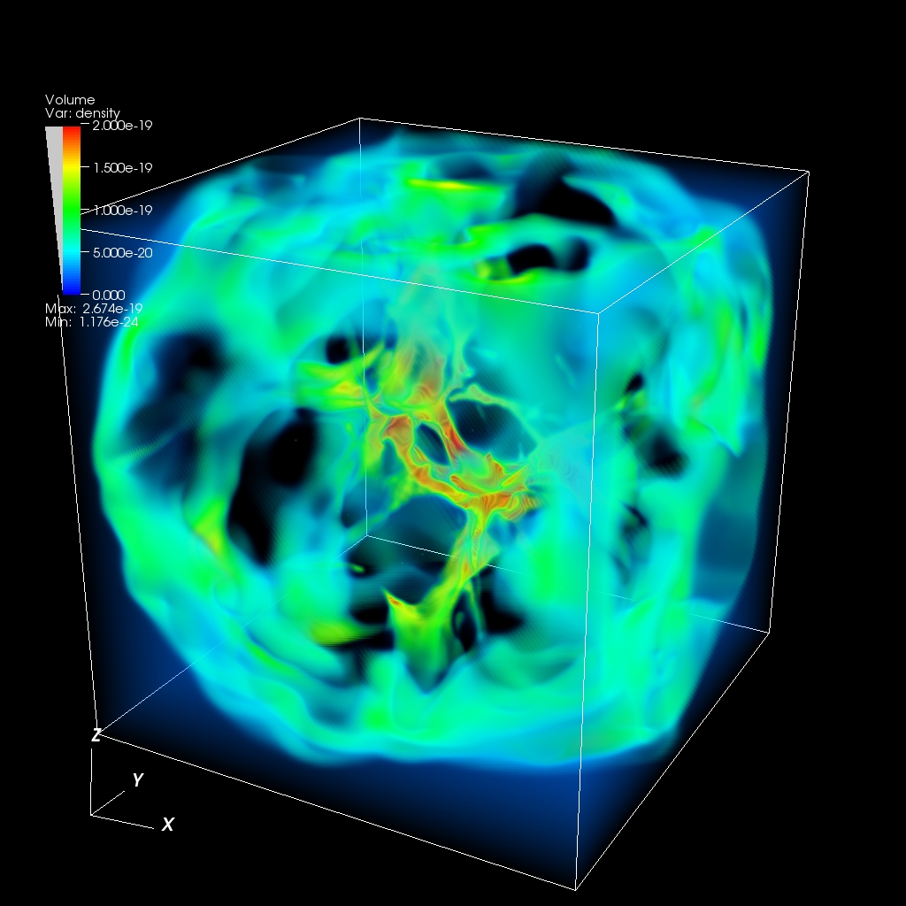
Figure 2.— Volume rendition of the density structure of model M1 after a $t=1.9\times 10^{5}$ yr time-integration. The grey-scale (color-scale in the online version) shows the density values in g cm^-3, linearly scaled, with an opacity that is also linearly proportional to the density. The cubic domain has a size of 1.2 pc.

In Figure 3, we show column density maps (obtained by integrating the number density along the $z$-axis of the computational domain) at integration times $t=19$, 3.2, 11 and $3.2\times 10^{4}$ yr for models M1, M2, M3 and M4, respectively. These times have been chosen so that the outer, dense shell is starting to leave the computational domain in each of the models. All of the maps have a central condensation, which has a peak column density of 9.11, 12.8, 66.6 and $36.3\times 10^{22}$ cm^-2 for models M1-M4, respectively.

Figure 4 shows column density maps for models M1-M4 computed only with the material from the ISM which originally permeated the computational domain. In these maps, the central condensation has a peak column density of 1.82, 10.8, 29.7 and $33.6\times 10^{22}$ cm^-2 for models M1-M4, respectively. Comparing the peak column densities for ISM material only (Figure 4) and the column densities for ISM+wind material (Figure 3), we see that while for model M1 the main contribution to the column density of the central condensation comes from the wind material, for models M2-M4 the main contribution to this column density comes from the material in the initial ISM.

We have also computed the fraction $f_{m}$ of mass of the initial ISM which is still present within the volume of the cluster (i. e., within a sphere of radius $R_{c}=0.5$ pc) for the time frames shown in Figure 4. We obtain $f_{m}=0.076$, 0.026, 0.26 and 0.052 for models M1-M4, respectively. Therefore, for model M3, almost 75% of the initial ISM mass has already been expelled from the volume of the cluster (most of this mass being present in the expanding shell pushed out by the cluster wind flow), and for the other three models more than 90 % of the ISM mass has been expelled.

As the material from the winds is unlikely to have dust, the column density distributions of the ISM material (see Figure 4) are proportional to the expected extinction. If we use a standard conversion factor $A_{V}=10^{-21}N_{H}$, where $A_{V}$ is the optical extinction and $N_{H}$ is the hydrogen column density in cm^-2, the peak values of $A_{V}$ corresponding to the central condensations are $A_{V}\approx 18$, 110, 300 and 340, for models M1-M4, respectively.

Finally, in Figure 5 we present a series of column density maps (computed only for the material of the initial ISM) illustrating the time-evolution obtained from model M3. From this time-sequence, we see that we can already identify the structure that forms the central condensation at $t=1.6\times 10^{4}$ yr. This condensation persists for $\sim 10^{5}$ yr (i. e., to the end of the time-integration). Several other features can be seen in both the $t=4.8\times 10^{4}$ and $t=7.9\times 10^{4}$ yr frames, indicating that the filaments have lifetimes $\sim 10^{4}$ yr.

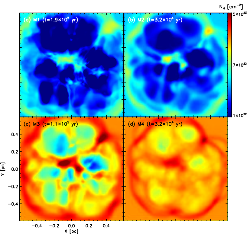
Figure 3.— Column density maps obtained from models M1-M4 by integrating the number density along the $z$-axis. The stratifications are shown with the logarithmic gray-scale (color-scale in the online version) given by the bar on the top right plot. The integration time for each model is indicated in the label at the top of each panel.

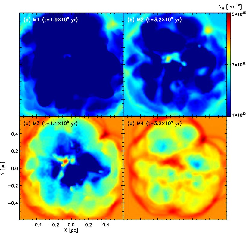
Figure 4.— ISM column density maps obtained from models M1-M4 by integrating the number density of the material in the initial ISM along the $z$-axis. The stratifications are shown with the logarithmic gray-scale (color-scale in the online version) given by the bar on the top right plot. The integration time for each model is indicated in the label at the top of each panel.

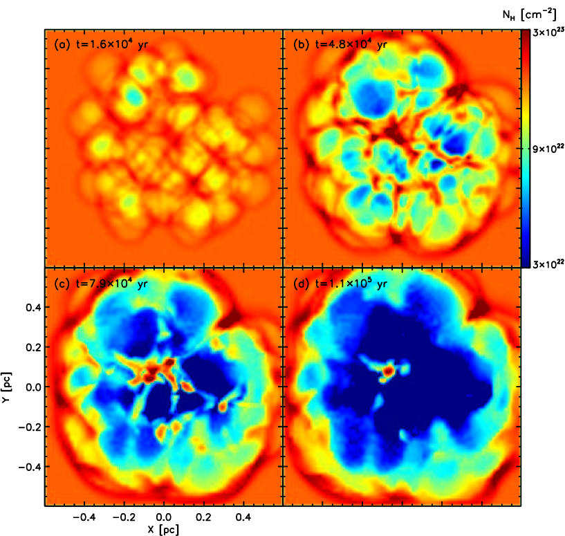
Figure 5.— Time-sequence showing the evolution of the ISM column density structure of model M3 (obtained by integrating the density of the material in the initial ISM along the $z$-axis). The stratifications are shown with the logarithmic gray-scale (color-scale in the online version) given by the bar on the top right plot.

4. Conclusions

Recent Spitzer observations of a young cluster of Herbig Ae/Be stars (Vig et al. 2007) show that the IR extinction towards IRAS 18511+0146 has a curious structure of filaments and clumps. This observation has motivated us to study the formation of dense, neutral structures as a result of the interaction between the winds of the young stars.

We find that if the Herbig Ae/Be stars have wind velocities $v_{w}<200$ km s^-1, the stellar wind interactions between nearby stars are highly radiative for mass loss rates as low as ${\dot{M}}_{w}\approx 3\times 10^{-7}$M_⊙yr^-1 (see Figure 1 and equation 5). However, for higher wind velocities, considerably higher mass loss rates are required for the wind interactions to be radiative. For example, for $v_{w}=400$ km s^-1, mass loss rates ${\dot{M}}_{w}>10^{-5}$M_⊙yr^-1 are required (see Figure 1). The values quoted in this paragraph are for an average separation of 0.1 pc between the stars in the cluster.

These values indicate that in a cluster of Herbig Ae/Be stars many of the wind interactions between nearby stars are likely to be in the highly radiative regime. We then compute a 3D simulation of a cluster wind flow in this regime, and we show that it does lead to the production of a structure of dense filaments and clumps.

From our simulations, we obtain predicted column density maps which show spatial structures which are qualitatively similar to the observations of IRAS 18511+0146 (Vig et al. 2007). Both the predicted and the observed maps show a structure of dense clumps and filaments, distributed within as well as outside the volume of the clump. We find that in all simulations a central clump is produced, which has a lifetime of $\sim 10^{5}$ yr.

It is more difficult to carry out a more quantitative comparison between our predictions and the observations of IRAS 18511+0146. Vig et al. (2007) first suggest that the filament/clump structures in this object have $A_{V}\sim 6$-$8$ extinctions (deduced from their Spitzer IR observations). However, when they compare these values with the extinction deduced from millimetre observations, they conclude that the IR maps probably have a strong contribution from foreground emission, and that the real values of the extinction should be $A_{V}\sim 50$. Therefore, only our model M1 produces visual extinctions which are too low compared with the ones deduced from the observations.

We end by noting that the simulation presented in this paper is the first attempt that has been made for modelling the interaction of the outflows from a cluster of young, low and intermediate mass stars. Our simulation was done assuming that :

• the stellar winds are “turned on” simultaneously,

• the region is initially filled by a homogeneous medium,

• the stellar outflows are isotropic,

• all of the stellar winds are identical.

It is particularly important to remove this last approximation if one wants to model IRAS 18511+0146 in detail, as this cluster harbours the massive protostar IRAS 18511 A.

The other assumptions in our models (listed above) are also not realistic, and the effects of removing them should be explored in future work. For example, assuming that the winds are isotropic is somewhat dubious in the context of a cluster of young stars. The more massive stars in such a cluster will evolve faster from an early, collimated outflow phase into a later phase in which a more isotropic wind is produced. The lower mass stars in the cluster will evolve less rapidly, and will remain in a collimated outflow phase for a longer period. For example, for a cluster with an age of $\sim 10^{5}$ yr one might expect to have a few more massive ($\sim 10$M_⊙) stars with isotropic winds, and a larger number of lower mass stars still producing jets. This combination of isotropic and collimated winds will result in flow configurations that might be applicable when more detailed observations of the wind interaction in clusters of young stars become available.

Another point that would be worthwhile to explore is the effect of the cooling function. As we have described in §2, our simulations are computed with a parametrized cooling function appropriate for partially (or fully) ionized gas. If one included a description of the non-equilibrium chemistry, and used it to compute a molecular cooling function, one would obtain cooling to lower temperatures in the dense filaments of compressed cloud material. This would lead to the production of narrower and denser filaments. A calculation including these effects should also have a substantially higher resolution in order to be able to resolve the associated cooling regions.

The conclusion that we obtain from the work described above is that the filamentary structure observed in IRAS 18511+0146 by Vig et al. (2007) might be the result of the surrounding ISM being compressed into dense sheets by the wind interactions between the cluster stars. However, it is of course clear that at least part of the observed structures could have been present initially in the dense cloud from which the cluster stars were formed.

References

- Canto et al. (2000) Cantó, J., Raga, A.C. & Rodríguez, L.F., 2000, ApJ, 536, 896.
- Chevalier & Clegg (1985) Chevalier, R.A. & Clegg, A.W.,1985, Nature, 317, 44.
- Hartigan, Raymond & Hartmann (1987) Hartigan, P., Raymond, J.& Hartmann, L., 1987, ApJ, 316, 323.
- Raga et al. (2000) Raga, A. C., Navarro-González, R., & Villagrán-Muniz, M. 2000, Revista Mexicana de Astronomia y Astrofisica, 36, 67.
- Raga et al. (2001) Raga, A.C., Velazquez, P.F., Cantó, J., Masciadri, E. & Rodríguez, L.F., 2001, ApJ, 559, L33.
- Raga & Reipurth (2004) Raga, A. C., Reipurth, B. 2004, RMxAA, 40, 15
- Raga et al. (2002) Raga, A. C., de Gouveia Dal Pino, E. M., Noriega-Crespo, A., Mininni, P. D., & Velázquez, P. F. 2002, A & A, 392, 267.
- Rodriguez-Gonzalez et al. (2007) Rodríguez-González, A., Cantó, J., Esquivel, A., Raga, A. C. & Velazquez, P. F., 2007, MNRAS, 380, 1198.
- Rockefeller et al. (2005) Rockefeller, G., Fryer, C. L., Melia, F., Wang, Q. D., 2005, ApJ, 623, 171.
- Silich et al. (2004) Silich, S., Tenorio-Tagle, G. & Rodríguez-González, A., 2004, ApJ, 610, 226.
- Tenorio-Tagle et al. (2005) Tenorio-Tagle,G., Silich, S., Rodríguez-González, A. & Muñoz-Tuñón, C., 2005, ApJ, 628, 13.
- Testi et al. (1999) Testi, L., Palla, F., Natta, A. 1999, A&A, 342, 515.
- Testi et al. (1997) Testi, L., Palla, F., Prusti, T., Natta, A., Maltagliati, S. 1997, A&A, 320, 159.
- Vig et al. (2007) Vig, S., Testi, L., Walmsley, M., Molinari, S., Carey, S., Noriega-Crespo, A. 2007, A&A, 470, 977.