Bypassing Cowling’s theorem in axisymmetric fluid dynamos

Abstract

We present a numerical study of the magnetic field generated by an axisymmetrically forced flow in a spherical domain. At small enough Reynolds number, $Re$, the flow is axisymmetric and generates an equatorial dipole above a critical magnetic Reynolds number $Rm_{c}$. The magnetic field thus breaks axisymmetry, in agreement with Cowling’s theorem. This structure of the magnetic field is however replaced by a dominant axial dipole when $Re$ is larger and allows non axisymmetric fluctuations in the flow. We show here that even in the absence of such fluctuations, an axial dipole can also be generated, at low $Re$, through a secondary bifurcation, when $Rm$ is increased above the dynamo threshold. The system therefore always find a way to bypass the constraint imposed by Cowling’s theorem. We understand the dynamical behaviors that result from the interaction of equatorial and axial dipolar modes using simple model equations for their amplitudes derived from symmetry arguments.

It is strongly believed that magnetic fields of planets and stars are generated by dynamo action, i.e., self generation of a magnetic field by the flow of an electrically conducting fluid moffatt. Planets and stars being rapidly rotating, axisymmetric flows about the axis of rotation have often been considered in order to work out simple dynamo models dudley . A major setback of the subject followed the discovery of Cowling’s theorem, which stated that a purely magnetic field cannot be maintained by dynamo action cowling . However, it has been shown that magnetic fields with a dominant axisymmetric mean part can be generated when non-axisymmetric helical fluctuations are superimposed to a mean axisymmetric flow alpha . This has been recently observed in the VKS experiment VKS . A strongly turbulent swirling von Kármán flow driven by two counter-rotating coaxial disks in a cylindrical container self-generated a magnetic field with a dipole mean component along the axis of rotation. This has been ascribed to an alpha effect due to the helical nature of the radially ejected flow along the two impellers petrelis07 . In this letter, we show that there exists another mechanism for bypassing the constraint imposed by Cowling’s theorem, without the help of non axisymmetric turbulent fluctuations. The mechanism is as follows: the primary dynamo bifurcation breaks axisymmetry in agreement with Cowling’s theorem. Then, the Lorentz force generates a non axisymmetric flow component which can drive an axisymmetric magnetic field through a secondary bifuraction. We show that direct numerical simulations confirm this scenario and that the two successive bifurcation thresholds can be very close in some flow configurations. The existence of two competing instability modes, the axial and equatorial dipoles, can lead to complex dynamical behaviors. Using symmetry arguments, we write equations for the amplitude of these modes that are coupled through the non axisymmetric velocity component. We show that the observed bifurcation structure and the resulting dynamics can be understood in the framework of this simple model.
We first numerically integrate the MHD equations in a spherical geometry for the solenoidal velocity $\bf v$ and magnetic $\bf B$ fields,

$$\frac{\partial\bf{v}}{\partial t}+(\bf{v}\cdot\mbox{\boldmath$\nabla$})\bf{v}\! = \!-\mbox{\boldmath$\nabla$}\pi+\nu\Delta\bf{v}+\bf{f}+\frac{1}{\mu\rho}(\bf{B}\cdot\mbox{\boldmath$\nabla$})\bf{B},$$ (1)

$$\frac{\partial\bf{B}}{\partial t}\! = \!\mbox{\boldmath$\nabla$}\times\left(\bf{v}\times\bf{B}\right)+\eta\,\Delta\bf{B}.$$ (2)

In the above equations, $\rho$ is the density, $\mu$ is the magnetic permeability and $\sigma$ is the conductivity of the fluid. The forcing is ${\bf f}=f_{0}\,{\bf F}$, where $F_{\phi}=s^{2}\sin(\pi\,s\,b)\,,\;F_{z}=\varepsilon\,\sin(\pi\,s\,c)\,,$ for $z>0$, using polar coordinates $(s,\phi,z)$ (normalized by the radius of the sphere $a$) and opposite for $z<0$. $F_{\phi}$ generates counter-rotating flows in each hemisphere, while $F_{z}$ enforces a strong poloidal circulation. The forcing is only applied in the region $0.25a<\mid\!z\!\mid<0.65a$, $s<s_{0}$. In the simulations presented here, $s_{0}=0.4$, $b^{-1}=2s_{0}$ and $c^{-1}=s_{0}$. This forcing has previously been introduced to model the mechanical forcing due to co-axial rotating impellers used in the Madison experiment bayliss07 . Although performed in a spherical geometry, this experiment involves a mean flow with a similar topology to that of the VKS experiment. Such flows correspond to $s_{2}+t_{2}$ flows in the Dudley and James classification dudley , i.e. two poloidal eddies with inward flow in the mid-plane, together with two counter-rotating toroidal eddies. We solve the above system of equations using the Parody numerical code parody . This code was originally developped in the context of the geodynamo (spherical shell) and we have here modified the code to make it suitable for a full sphere. We use the same dimensionless numbers as in bayliss07 , the magnetic Reynolds number $Rm=\mu_{0}\sigma a\,{\rm max}(|\bf v|)$, and the magnetic Prandtl number $Pm=\nu\mu_{0}\sigma$. The kinetic Reynolds number is then $Re=Rm/Pm$.

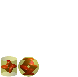
Figure 1: Comparison of the magnetic field generated by an axisymmetric $s2+t2$ flow in different geometries. Isovalue of the magnetic energy in a cylinder (from Kris1 ) or a sphere.

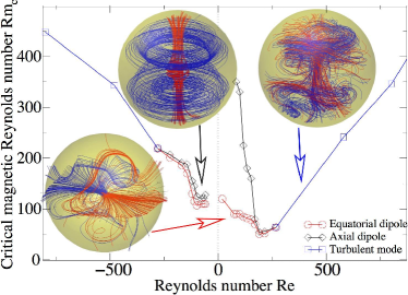
Figure 2: Stability curves $Rm_{c}=f(Re)$ obtained with direct numerical simulations. In red: onset of the $m=1$ (equatorial dipole) dynamo mode; black: non-linear threshold of the $m=0$ (axisymmetric) mode; in blue the turbulent mode emerging from velocity fluctuations. The corresponding magnetic structures are represented using magnetic field lines.

The dynamo threshold $Rm_{c}$ is displayed as a function of $Re$ in Fig. 2. Negative $Re$ corresponds to a flow that is reversed compared to the VKS configuration, i.e. directed from the impellers to the center of the flow volume along the axis and radially outward in the mid-plane. For small enough $Re$, the flow is laminar and axisymmetric. A magnetic field with a dominant equatorial dipole mode $m=1$ is generated first (red curve in Fig. 2). The geometry of the field is displayed in the left inset of Fig. 2 and breaks axisymmetry as expected from Cowling’s theorem. This dynamo mode is similar to that obtained in cylindrical geometry, as illustrated in Fig 1.

For $Re$ larger than about $300$, the flow becomes turbulent and the equatorial dipole is then replaced by a dominant axisymmetric mode $m=0$. Its threshold increases with $Re$ in the parameter range of the simulations (blue curve in Fig. 2 and its geometry is shown in the right inset). These results are in agreement with bayliss07 . It is remarkable that the axial dipole observed in the VKS experiment and ascribed to non axisymmetric fluctuations petrelis07 can also be obtained in the present simulations even though the level of fluctuations is much smaller (the parameter range realized in the experiment being, by far, out of reach of present computer models).

In addition, an axisymmetric magnetic field can also be generated at very low $Re$ through a secondary bifurcation from the equatorial dipole when $Rm$ is increased. This corresponds to the black curves in Fig. 2. The corresponding mode is shown in the top left inset of Fig. 2. Bifurcation diagram of Fig. 3 helps to understand the mechanism by which this axisymmetric magnetic field is generated. One can observe that the equatorial dipole first bifurcates supercritically for $Rm=88$ when $Re=+122$. The back-reaction of the Lorentz force is twofold. First, it inhibits the axisymmetric velocity field, which decreases (orange curve in Fig. 3). Second, and more importantly, it drives a non-axisymmetric $m=2$ velocity mode (blue curve in Fig. 3). Once the intensity of this flow becomes strong enough, it yields a secondary bifurcation of the axisymmetric $m=0$ field mode. This is achieved for $Rm=205$ (black curve in Fig. 3). The amplitude of the equatorial dipole decreases immediately after this secondary bifurcation. We observe that the $m=0$ mode vanishes at higher $Rm$ and then grows again above $Rm=425$. Although the amplitude of the equatorial and axial modes behave in a complex manner as $Rm$ is increased, we observe that they are anti-correlated, thus showing that they inhibit each other through the non-linear couplings.

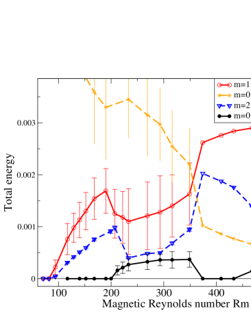
Figure 3: Bifurcation diagram of different magnetic modes varying $Rm$ with fixed $Re=+122$. Error bars indicate the amplitude of oscillations. All other magnetic modes are very small compared to these ones.

For $Re<0$, Fig. 2 shows that the primary and secondary bifurcations occur in a much narrower range of $R_{m}$. The equatorial dipole mode is then close to marginal stability when the axial one bifurcates, and their nonlinear interactions leads to complex time dependent dynamics close to threshold as displayed in Fig. 4.

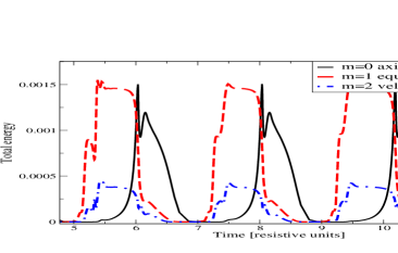
Figure 4: Time recordings of the total energy of the equatorial and axial dipolar modes, and of the $m=2$ velocity mode for $Re=-76$ and $Rm=170$.

Figure 5: Bifurcation diagram of different magnetic modes varying $Rm$ at fixed $Re=-76$. Error bars indicate the amplitude of oscillations. Dashed lines correspond to the maximum values of the different modes in the relaxation regime. All other magnetic modes are very weak compared to these ones.

The equatorial mode (red curve) is generated first and saturates, but it drives the axial mode (black curve) through the non axisymmetric part of the velocity field. The axial dipole then inhibits the equatorial one that decays almost to zero. As a result, the flow is no longer driven away from axisymmetry by the Lorentz force. The axial dipole thus decays and the process repeats roughly periodically. We observe that during one part of the cycle, the magnetic field is almost axisymmetric. It involves a strong azimuthal field together with a large vertical component near the axis of rotation, i.e. an axial dipole (see the left inset of Fig. 2). These relaxation oscillations, present only in the $Re<0$ case, occur only slightly above the threshold of the secondary bifurcation of the $m=0$ mode. Their period first decreases when $Rm$ is increased, but then increases showing a divergence when the relaxation oscillations bifurcate to a stationary regime, as displayed in figure 5. Above this transition, we observe bistability with the coexistence of two solutions: a nearly equatorial dipole, with a strong equatorial component and a weak axial one (labeled $M_{1}$ in figure 5) and a nearly axial dipole (labeled $M_{2}$).

We will show next that this competition between equatorial and axial modes, and the resulting dynamics, can be understood using a simple model for the amplitudes of the relevant modes. We thus write

$${\bf B}({\bf r},t)=A(t)\,{\bf D}_{eq}({\bf r})+c.c.+B(t)\,{\bf D}_{ax}({\bf r})+\cdots,$$ (3)

where ${\bf D}_{eq}({\bf r})$ (respectively ${\bf D}_{ax}({\bf r})$) is the eigenmode related to the equatorial (respectively axial) dipole. $A$ is a complex amplitude, its phase describes the angle of the dipole in the equatorial plane and $c.c.$ stands for the complex conjugate of the previous expression. $B$ is a real amplitude. As said above, the equatorial dipole ($m=1$) generates a non axisymmetric flow through the action of the Lorentz force. The later depends quadratically on the magnetic field, this non axisymmetric velocity mode of complex amplitude $V(t)$ thus corresponds to $m=2$. Using symmetry arguments, i.e., rotational invariance about the $z$–axis which implies the invariance of the amplitude equations under $A\rightarrow A\exp i\chi,V\rightarrow V\exp 2i\chi$, and the ${\bf B}\rightarrow-{\bf B}$ symmetry, we get up to the third order

$$\dot{A} = \mu A-V\overline{A}-\alpha_{1}{\mid\!A\!\mid}^{2}A-\alpha_{2}{\mid\!V\!\mid}^{2}A-\alpha_{3}B^{2}A\,,$$ (4)

$$\dot{V} = -\nu V+A^{2}-\beta_{1}{\mid\!A\!\mid}^{2}V-\beta_{2}{\mid\!V\!\mid}^{2}V-\beta_{3}B^{2}V\,,$$ (5)

$$\dot{B} = -\lambda B-\gamma_{1}{\mid\!A\!\mid}^{2}B+\gamma_{2}{\mid\!V\!\mid}^{2}B-\gamma_{3}B^{3}\,.$$ (6)

$\mu$ is proportional to the distance to the dynamo threshold. Clearly $\nu>0$, since the flow is axisymmetric below threshold. The coefficients of the quadratic terms can be scaled by an appropriate choice of the amplitudes. The term $A^{2}$ represents the forcing of the non axisymmetric flow by the Lorentz force related to the equatorial dipole. $V\overline{A}$ means that rotational invariance for the equatorial dipole is broken as soon as a non axisymmetric flow is generated. We have fixed its sign so that the bifurcation of the equatorial dipole remains supercritical $\forall\alpha_{1}\geq 0$. The equations for $A$ and $V$ (with $B=0$) are the normal form of a $1:2$ resonance resonance1-2 and have been studied in details in other contexts. In particular, it is known that this system can undergo a secondary bifurcation for which the phase of $A$ begins to drift at constant velocity when $\mu$ reaches a value such that ${\mid\!A\!\mid}^{2}=2{\mid\!V\!\mid}^{2}$. This corresponds here to a rotating dipole, at constant rate, in the equatorial plane. Consider now the equation for the amplitude $B$ of the axial magnetic field. Taking $\lambda>0$ and $\gamma_{3}>0$ ensures that it cannot be generated alone, in agreement with Cowling’s theorem. The term ${\mid\!V\!\mid}^{2}B$ describes the possible amplification of $B$ from the non axisymmetric velocity field provided that $\gamma_{2}>0$. Although the system of amplitude equation (4-5-6) cannot be derived asymptotically from (1, 2), it reproduces the phenomenology observed with the direct simulations for both signs of $Re$: when $\mu$ is increased, we either obtain relaxation oscillations as for $Re<0$ (parameters of fig. 6) or a secondary bifurcation of the axial field as for $Re>0$ (same parameters with $\gamma_{2}=1$). The relaxation oscillations are displayed in Fig. 6 (left). The model helps to understand the qualitative features observed in the direct simulation: it involves a solution corresponding to an equatorial dipole ($A_{0},V_{0},B=0$) that can bifurcate to a mixed mode $(A_{1},V_{1},B_{1})$ involving a non zero axial field. In addition, two types of mixed modes can exist, one with a dominant equatorial dipole, say $M_{1}=(A_{1},V_{1},B_{1})$, and another with a dominant axial dipole $M_{2}=(A_{2},V_{2},B_{2})$. Depending on the stability of these two solutions, we observe either one of the mixed mode (depending on initial conditions), or a relaxation oscillation slowing down in the vicinity of these unstable fixed points and the origin. The system thus has three fixed points with both stable and unstable directions: the origin where both modes are zero, a point with a dominant equatorial dipole and a point with a dominant axial dipole. This situation leads to a heteroclinic cycle connecting these three unstable equilibrium points and corresponds to the relaxation oscillations (see fig. 6, right) .

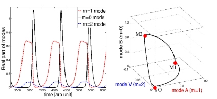
Figure 6: Numerical integration of the amplitude equations (4-5-6). Left: time recordings of the amplitudes of the equatorial and axial magnetic modes interacting through the non axisymmetric velocity mode ( $\mu=1,\alpha_{1}=0.3,\alpha_{3}=4,\nu=0.5,\beta_{2}=1.5,\lambda=1.8,\gamma_{1}=0.5,\gamma_{2}=10,\gamma_{3}=0.5$, all other coefficients being zero.) Right: relaxation cycle in phase space involving the three unstable fixed points (real part of $A$, $V$).

In sodium flows driven by an axisymmetric forcing, such as the ones used in the VKS VKS , Madison and Maryland experiments USboys , one expects a possible competition between equatorial and axial dynamo modes. Indeed, the mean flow, if it were acting alone, would generate an equatorial dipole in agreement with Cowling’s theorem. Our direct simulations show that a fairly small amount of non axisymmetric fluctuations (compared to the experiments) is enough to drive an axial ($m=0$) dipole as observed in the VKS experiment for the mean magnetic field. In addition, we show here that even without turbulent fluctuations, the non axisymmetric flow driven by the Lorentz force related to the equatorial dipole, can generate the axial one through a secondary bifurcation. The equatorial dipole can easily rotate in the equatorial plane, thus averaging to zero. The axial dipole then becomes the dominant part of the mean magnetic field.

It is striking that this mechanism that generates an axial dipole occurs much closer to the dynamo threshold when we go from the $Re>0$ to the $Re<0$ flow configuration, thus when the product of the helicity times the differential rotation is changed to its opposite value. For $Re<0$, the shear layer in the mid-plane becomes favorable to an $\alpha-\omega$ dynamo as soon as the axisymmetry of the flow is broken. For $Re>0$, the flow near the impellers can play a similar role but the effect is weaker. This opens interesting perspectives for flows that can be used for future dynamo experiments: an $\alpha-\omega$ effect driven by the strong vortices present in the shear layer close to the mid-plane can be favored by the $Re<0$ configuration. To wit, one can use either the optimized set-up described in petrelis07 or propellors with the appropriate pitch in the VKS or Madison experiments.

A competition between equatorial and axial dipolar modes could also account for secular variations of the Earth magnetic field. It would be interesting to check whether some features can be described with a low dimensional model similar to the one used in this study.