Transitional solar dynamics, cosmic rays and global warming

Abstract

Solar activity is studied using a cluster analysis of the time-fluctuations of the sunspot number. It is shown that in an Historic period the high activity components of the solar cycles exhibit strong clustering, whereas in a Modern period (last seven solar cycles: 1933-2007) they exhibit a white-noise (non-)clustering behavior. Using this observation it is shown that in the Historic period, emergence of the sunspots in the solar photosphere was strongly dominated by turbulent photospheric convection. In the Modern period, this domination was broken by a new more active dynamics of the inner layers of the convection zone. Then, it is shown that the dramatic change of the sun dynamics at the transitional period (between the Historic and Modern periods, solar cycle 1933-1944yy) had a clear detectable impact on Earth climate. A scenario of a chain of transitions in the solar convective zone is suggested in order to explain the observations, and a forecast for the global warming is suggested on the basis of this scenario. A relation between the recent transitions and solar long-period chaotic dynamics has been found. Contribution of the galactic turbulence (due to galactic cosmic rays) has been discussed. These results are also considered in a content of chaotic climate dynamics at millennial timescales.

I Introduction

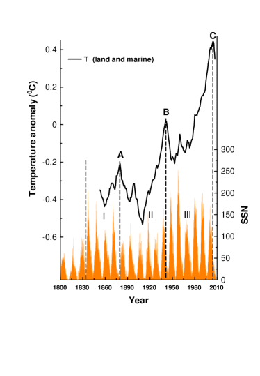
Figure 1: Sunspot number (SSN, monthly) vs time belg . The dashed straight lines separate between periods of different intensity of the solar activity. The solid curve shows the global temperature anomaly (combined land and marine, 7-years running average) temp .

The sunspot number is the main direct and reliable source of information about the solar dynamics for historic period. This information is crucial, for instance, for analysis of a possible connection between the sun activity and the global warming. In a recent papers sol ,usos1 results of a reconstruction of the sunspot number were presented for the past 11,400 years. The reconstruction shows that sol : ”..the level of solar activity during the past 70 years is exceptional, and the previous period of equally high activity occurred more than 8,000 years ago” (section III in Fig. 1) .

Figure 1 gives first indication (’by eye’), that the prominent maxima of the global temperature data (solid curve in the Fig. 1) correspond to transitions between periods of different intensity of the Sun activity (characterized by the monthly sunspot number-SSN). This observation can be considered as an indication of a strong impact of the solar activity transitions on the global Earth climate. Therefore, understanding of the physical processes in the Sun, which cause these activity transitions, seems to be crucial for any serious forecast for global Earth climate.

II Sunspots

When magnetic field lines are twisted and poke through the solar photosphere the sunspots appear as the visible counterparts of magnetic flux tubes in the convective zone of the sun. Since a strong magnetic field is considered as a primary phenomenon that controls generation of the sunspots the crucial question is: Where has the magnetic field itself been generated? The location of the solar dynamos is the subject of vigorous discussions in recent years. A general consensus had been developed to consider the shear layer at the bottom of the convection zone as the main source of the solar magnetic field sw (see, for a recent review brand1 ). In recent years, however, the existence of a prominent radial shear layer near the top of the convection zone has become rather obvious and the problem again became actual. The presence of large-scale meandering flow fields (like jet streams), banded zonal flows and evolving meridional circulations together with intensive multiscale turbulence shows that the near surface layer is a very complex system, which can significantly affect the processes of the magnetic field and the sunspots generation. There could be two sources for the poloidal magnetic field: one near the bottom of the convection zone (or just below it sw ), another resulting from an active-region tilt near the surface of the convection zone. For the recently renewed Babcock-Leighton bab ,leig solar dynamo scenario, for instance, a combination of the sources was assumed for predicting future solar activity levels dtg , ccj . In this scenario the surface generated poloidal magnetic field is carried to the bottom of the convection zone by turbulent diffusion or by the meridional circulation. The toroidal magnetic field is produced from this poloidal field by differential rotation in the bottom shear layer. Destabilization and emergence of the toroidal fields (in the form of curved tubes) due to magnetic buoyancy can be considered as a source of pairs of sunspots of opposite polarity. The turbulent convection in the convection zone and, especially, in the near-surface layer captures the magnetic flux tubes and either disperses or pulls them trough the surface to become sunspots.

The magnetic field plays a passive role in the photosphere and does not participate significantly in the turbulent photospheric energy transfer. On the other hand, the very complex and turbulent near-surface layer (including photosphere) can significantly affect the process of emergence of sunspots. The similarity of light elements properties in the spot umbra and granulation is one of the indication of such phenomena.

The present paper reports a direct relation between the fluctuations in sunspot number and the temperature of photospheric turbulent convection in the Historic period. This relation allows for certain conclusions about the generation mechanisms of the magnetic fields and the sunspots. In the Modern period (section III in Fig. 1, cf. sol ,usos1 ) the relative role of the surface layer (photosphere) in the process of emergence of sunspots decreased in comparison with the Historic period (section II in Fig. 1), implying a drastic increase of the relative role of the inner layers of the convection zone in the Modern period.

III Time-clustering of fluctuations

In order to extract new information from sunspot number data we apply the fluctuation clustering analysis suggested in the Ref. sb (see also Ref. bEPL ). For a time depending signal we count the number of ’zero’-crossings of the signal (the points on the time axis where the signal is equal to zero) in a time interval $\tau$ and consider their running density $n_{\tau}$. Let us denote fluctuations of the running density as $\delta n_{\tau}=n_{\tau}-\langle n_{\tau}\rangle$, where the brackets mean the average over long times. We are interested in scaling variation of the standard deviation of the running density fluctuations $\langle\delta n_{\tau}^{2}\rangle^{1/2}$ with $\tau$

$$\langle\delta n_{\tau}^{2}\rangle^{1/2}\sim\tau^{-\alpha}$$

For white noise signal it can be derived analytically molchan ,lg that $\alpha=1/2$ (see also sb ). The same consideration can be applied not only to the ’zero’-crossing points but also to any level-crossing points of the signal.

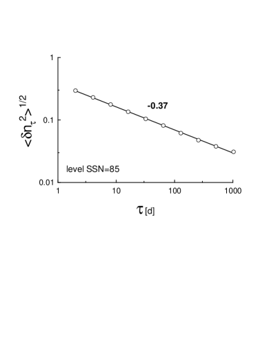
Figure 2: The standard deviation for $\delta n_{\tau}$ vs $\tau$ (Historic period) in log-log scales. The straight line (the best fit) indicates the scaling law Eq. (1).

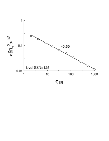
Figure 3: The standard deviation for $\delta n_{\tau}$ vs $\tau$ (Modern period) in log-log scales. The straight line (the best fit) indicates the scaling law Eq. (1).

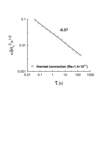
Figure 4: The standard deviation for $\delta n_{\tau}$ vs $\tau$ for the temperature fluctuations in the Rayleigh-Bernard convection laboratory experiment with $Ra=1.4\times 10^{11}$ ns . The straight line indicates the scaling law Eq. (1).

One can see that for the Modern period (section III in Fig. 1) the solar activity is significantly different from that for the Historic period (section II in Fig. 1). Therefore, in order to calculate the cluster exponent (if exists) for this signal one should make this calculation separately for the Modern and for the Historic periods. We are interested in the active parts of the solar cycles. Therefore, for the Historic period let us start from the level SSN=85. The set of the level-crossing points has a few large voids corresponding to the weak activity periods. In the telegraph signal Ref. [10], corresponding to the data set, the large voids became so clear detectable that there is no problem to cut them off. Then, the remaining data have been merged providing a statistically stationary set (about $10^{4}$ data points). The robustness of the procedure has been successfully checked.

Fig. 2 shows (in the log-log scales) dependence of the standard deviation of the running density fluctuations $\langle\delta n_{\tau}^{2}\rangle^{1/2}$ on $\tau$ for this data set. The straight line is drawn in this figure to indicate the scaling (1). The slope of this straight line provides us with the cluster-exponent $\alpha=0.37\pm 0.02$. This value turned out to be insensitive to a reasonable variation of the SSN level. Results of analogous calculations (including the large voids ’cut off’ procedure) performed for the Modern period are shown in Fig. 3 for the SSN level SSN=125. The calculations performed for the Modern period provide us with the cluster-exponent $\alpha=0.5\pm 0.02$ (and again this value turned out to be insensitive to a reasonable variation of the SSN level).

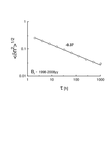
Figure 5: The standard deviation for $\delta n_{\tau}$ vs. $\tau$ for radial component $B_{r}$ of the interplanetary magnetic field, as measured by the ACE magnetometers for the last solar cycle (hourly average ACE ).

The exponent $\alpha\simeq 0.5$ (for the Modern period) indicates a random (white noise like) situation. While the exponent $\alpha\simeq 0.37$ (for the Historic period) indicates strong clustering. The question is: Where is this strong clustering coming from? It is shown in the paper sb that turbulence produces signals with strong clustering. Moreover, the cluster exponents for these signals depend on the turbulence intensity and they are nonsensitive to the types of the boundary conditions. Fortunately, we have direct estimates of the value of the main parameter characterizing intensity of the turbulent convection in photosphere: Rayleigh number $Ra\sim 10^{11}$ (see, for instance bld ). In Fig. 4 we show calculation of the cluster exponent for the temperature fluctuations in the classic Rayleigh-Bernard convection laboratory experiment for $Ra\sim 10^{11}$ (for a description of the experiment details see ns ). The calculated value of the cluster exponent $\alpha=0.37\pm 0.01$ coincides with the value of the cluster-exponent obtained above for the sunspot number fluctuations for the Historic period. The value of the Rayleigh number $Ra$ in the photosphere for the Historic period has the same order as for the Modern period: $Ra\sim 10^{11}$ (see next Section). Therefore, the photospheric temperature fluctuations can produce the strong clustering of the sunspot number fluctuations for the Historic period. This seems to be natural for the case when the photospheric convection determines the sunspot emergence in the photosphere. However, in the case when the effect of the photospheric convection on the SSN fluctuations is comparable with the effects of the inner convection zone layers on the SSN fluctuations the clustering should be randomized by the mixing of the sources, and the cluster exponent $\alpha\simeq 0.5$ (similar to the white noise signal). The last case apparently takes place for the modern period.

Since the Rayleigh number $Ra$ of the photospheric convection preserves its order $Ra\sim 10^{11}$ with transition from the Historic period to the Modern one (see next Section), we can assume that just significant changes of the dynamics of the inner layers of the convection zone (most probably - of the bottom layer) were the main reasons for the transition from the Historic to the Modern period.

IV Magnetic fields in the solar wind and on Earth

Although for the Modern period the turbulent convection in the photosphere has no decisive impact on the sunspots emergence, the large-scale properties of the magnetic field coming through the sunspots into the photosphere and then to the interplanetary space (so-called solar wind) can be strongly affected by the photospheric motion. In order to be detected the characteristic scaling scales of this impact should be larger than the scaling scales of the interplanetary turbulence (cf. b1 ,gold ). In particular, one can expect that the cluster-exponent of the large-scale interplanetary magnetic field (if exists) should be close to $\alpha\simeq 0.37$. In Fig. 5 we show cluster-exponent of the large-scale fluctuations of the radial component $B_{r}$ of the interplanetary magnetic field. For computing this exponent, we have used the hourly averaged data obtained from Advanced Composition Explorer (ACE) satellite magnetometers for the last solar cycle ACE . As it was expected the cluster-exponent $\alpha\simeq 0.37\pm 0.02$. Analogous result was obtained for other components of the interplanetary magnetic field as well.

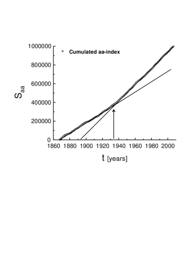
Figure 6: Cumulative aa-index vs. time. Daily aa-index was taken from wdc . The arrow indicates beginning of the transitional solar cycle.

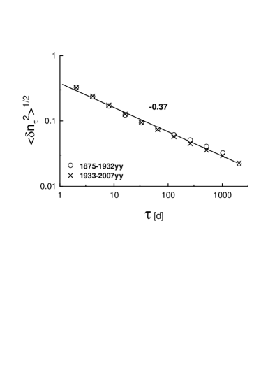
Figure 7: The standard deviation for $\delta n_{\tau}$ vs. $\tau$ (in log-log scales) for the daily aa-index wdc : circles correspond to the Historic period and crosses correspond to the Modern period.

At the Earth itself the solar wind induced activity is measured by geomagnetic indexes such as aa-index (in units of 1 nT). This, the most widely used long-term geomagnetic index may , presents long-term geomagnetic activity and it is produced using two observatories at nearly antipodal positions on the Earth’s surface. The index is computed from the weighted average of the amplitude of the field variations at the two sites. It was recently discovered that variations of this index are strongly correlated with the global temperature anomalies (see, for instance, cbf ,land ). In this paper, however, we will be mostly interested in the clustering properties of the aa-index and their relation to the modulation produced by the photospheric convective motion. The point is that the data for the aa-index are available for both the Modern and the Historic periods. This allows us to check the suggestion that the Rayleigh number of the photospheric convection has the same order for the both mentioned periods. The transition between the two periods can be seen in Figure 6, where we show the cumulated aa-index $a(t)$

$$S_{aa}(t)=\int_{0}^{t}a(t^{\prime})dt^{\prime}$$

The arrow in this figure indicates beginning of the transitional solar cycle.

Figure 7 shows cluster-exponents for both the Modern and the Historic periods calculated for the low intensity levels of the aa-index (for the Historic period the level used in the calculations is aa-index=10nT, whereas for the Modern period the level is aa-index=25nT, the aa-index was taken from wdc ). The low levels of intensity were chosen in order to avoid effect of the extreme phenomena (magnetic storms and etc.). The straight line in Fig. 7 is drawn to show the expected value of the cluster-exponent $\alpha\simeq 0.37$ for the both periods. It means that indeed for both the Historic and the Modern periods the Rayleigh number $Ra\sim 10^{11}$ (cf. Fig. 4) in the solar photosphere.

V Impact of the solar dynamics on Earth climate

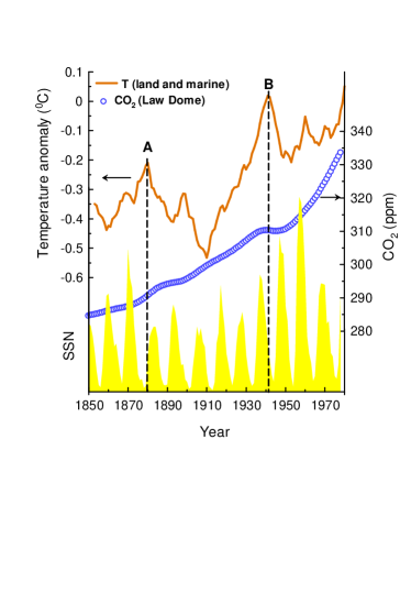
Figure 8: Global temperature anomaly (solid curve, combined land and marine) temp and atmospheric $CO_{2}$ (circles) lawdome vs time. Relevant daily SSN are also shown.

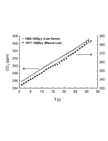
Figure 9: Comparison of the $CO_{2}$ growth for the periods 1900-1930yy lawdome and 1977-2008yy maunaloa . The solid straight lines (best fit) indicate a linear growth.

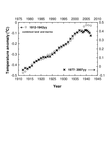
Figure 10: Comparison of the temperature anomaly (combined land and marine) temp for the periods 1912-1942yy and 1977-2007yy.

The transitions of the solar convection zone dynamics can affect the earth climate through (at least) two channels. First channel is a direct change in the heat and light output of the Sun, especially during the transitional solar cycle 1933-1944yy. Second channel is related to the strong increase of the magnetic field output in the interplanetary space through the sunspots. The interplanetary magnetic field interacts with the cosmic rays. Therefore, the change in the magnetic field intensity can affect the Earth climate through the change of the cosmic rays intensity and composition (see, for instance, Refs. uk ,shav ,kirk ). Let us look more closely to the transition B in Fig. 1. The Fig. 8 shows global temperature anomaly (the solid curve) temp and atmospheric $CO_{2}$ mixing ratios (the circles) lawdome vs. time. Relevant SSNs are also shown. The dashed straight line (corresponding to the peak B) separates between Historic and Modern periods. One can see, that the transitional solar cycle (1933-1944yy) is characterized by dramatic changes both in the global temperature (a huge peak) and in the atmospheric $CO_{2}$ (complete suppression of the growth). After the transitional period one can observe (during the three solar cycles: 1944-1977yy) certain growth in the temperature anomaly and an unusually fast growth in the atmospheric $CO_{2}$. These three solar cycles seems to be an aftershock adaptation of the global climate to the new conditions. Then, starting from 1977 year, the atmospheric $CO_{2}$ growth returns to its linear trend as before the transition B, but now the rate of the growth is about four times larger than before the transition (see Fig. 9). On the other hand, it can be seen from Fig. 1 that the temperature anomaly before the maximum C returns to about the same growth pattern as it was just before the transition B. A quantitative comparison of these patterns, shown in Figure 10, indicates only about 20% difference in the growth rate (cf. also Refs. ah , gt ). The thirty year periods used for this comparison could find a support in the Appendix B.

If one consider the impact mechanism, related to the energetic cosmic (charged) particles and the corresponding screen effect of the magnetic fields, one could expect that this impact mechanism should be also sensitive to the 11-year solar cycle variability (though considerably less than to the transitional effects). To find fingerprints of this variability in the global temperature anomaly data is not a trivial task due to comparatively (to the 11-year cycle) short period of observations and due to the statistically non-stationary character of these data (with considerable time trends). To extract these fingerprints we will use a time series decomposition method developed in ks ,bd ,k . A time series is decomposed into a trend (like that shown in Fig. 1 as the solid curve) and a fluctuating (noise-like) components (see Appendix A). The method applies state space modeling and Kalman filter. Parameters are estimated by maximum likelihood method. Obtained by this way the fluctuating (noise-like) component of the (filtered) signal presents a statistically stationary time series and, therefore, it can be subject of a spectral analysis. Result of this analysis for the global temperature anomaly (combined land and marine temp ) is shown in Figure 11. Although we have deal with a comparatively short data series one can clear see the main spectral peak corresponding to the (about) 11-year solar cycle impact (cf. Refs. shav ,swest ,swest2 ). If one also introduces an autoregressive (AR) component into the time series decomposition (see Appendix A) to describe the fluctuating part of the global temperature anomaly, then one can compute energy spectrum of the AR component. Such spectrum is shown in figure 12. One can clear see the spectral peak corresponding to the solar 11-year cycle impact.

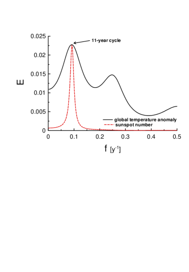
Figure 11: The solid curve corresponds to energy spectrum of the fluctuating (noise-like) component of the decomposed global temperature anomaly time series (combined land and marine temp ). The dashed curve corresponds to energy spectrum of fluctuating component of the SSN data.

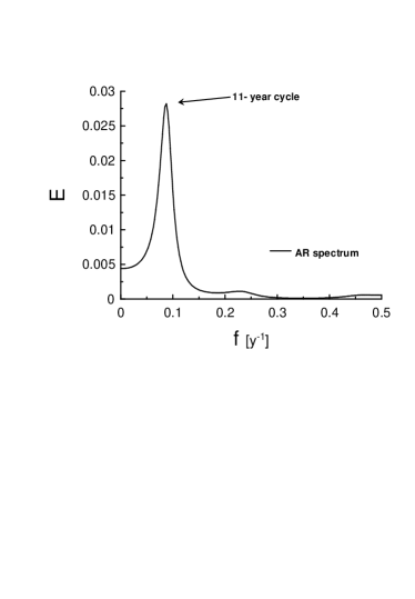
Figure 12: Energy spectrum of the AR (fluctuating) component of the decomposed global temperature anomaly time series (combined land and marine temp ).

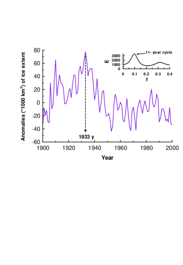
Figure 13: Trend of anomalies of ice August extent in the Chukchi sea pol2 . The insert shows spectrum of fluctuating (noise-like) component of the time series decomposition.

It is also interesting to look at the reduction in arctic ice extent. Figure 13 shows a trend component of the anomalies of ice August extent in the Chukchi sea (the data are taken from pol2 ) obtained by the time series decomposition. The dashed straight line indicates beginning of the transitional solar cycle. Insert to Fig. 13 shows spectrum of corresponding fluctuating (noise-like) component of the (filtered) signal (cf. Fig. 11). The dashed straight line indicates beginning of the transitional solar cycle. This arctic sea is located sufficiently far from the North Atlantic to diminish its influence, whereas influence of the Pacific ocean on the Chukchi sea local climate is not very significant.

VI A forecast

At present time we can already observe a peak C in the global temperature anomaly (see Fig. 1). The last observation can be considered as an indication of the current transition to a new section IV in the solar activity. The fact that in the ’last’ period (1977-2007yy) the temperature anomaly growth returned to the same pattern as just before the transition peak B (see Fig. 10) provides an additional support to this suggestion.

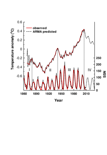
Figure 14: The upper solid curve corresponds to the observed yearly global temperature anomaly data (7-year smoothed) temp . The lower solid curve corresponds to the observed SSN data (year-smoothed) belg . The dashed curves are an ARMA-prediction: for SSN and for global temperature anomaly.

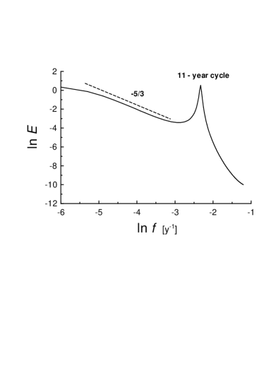
Figure 15: ARMA spectrum of the global temperature anomaly fluctuations in the ln-ln scales. The straight dashed line is drawn to indicate the Kolmogorov scaling law $E(f)\sim f^{(-5/3)}$.

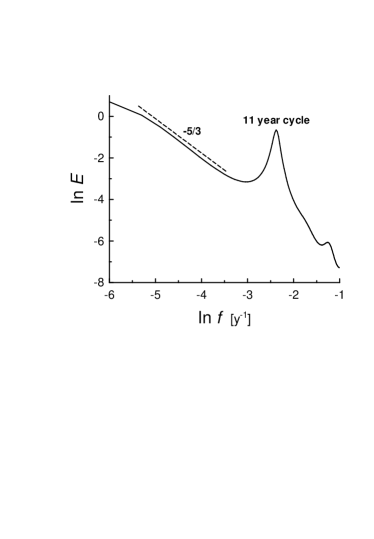
Figure 16: Spectrum of the galactic cosmic ray count rate fluctuations in the ln-ln scales (the reconstructed data for period 1611-2007yy have been taken from usos-recon ). The straight dashed line is drawn to indicate the Kolmogorov scaling law $E(f)\sim f^{(-5/3)}$.

To make a forecast for the new section IV let us assume that there was a storage of certain part of the energy coming from the radiative zone during the period of the section II (Fig. 1). Then, in the period of the section III this stored energy was released and transported to the Sun surface. This release was not in the form of the thermal convection, but in the form of strongly concentrated toroidal magnetic field structures, which results in the intense emergence of the sunspots in the active parts of the Modern period (section III in Fig. 1). It is interesting that the storage and release periods have about the same length: $\simeq 60$ years (see also Appendix B). The storage of energy in a growing magnetic field at the bottom of the convection zone or in the overshoot (by the convective downflows) area just under the bottom can be considered as the most plausible for this scenario. Convective overshooting provides means to store magnetic energy below the convection zone by resisting the buoyancy effect for large time scales. Level of subadiabaticity in the overshoot layer, needed in order to store the magnetic flux for sufficiently long times, can be significant. Expected intensity of $10^{5}~{}G$ results an energy density that is in order of magnitude larger than equipartition value. Though, suppression of convective motion by the magnetic flux tubes themselves can be considered as an additional factor allowing to achieve the sufficient level of subadiabaticity (see, for instance sw ,brand1 ,th ).

Since the section III in the solar activity was a release one, it is naturally to assume that the next section (IV) in the solar activity will be a ’storage’ one, similar to the ’storage’ section II. As for the corresponding Earth temperature anomaly, the section IV is also expected to be similar to the section II. But the temperature anomaly from the beginning of the section IV will be shifted upward on about $0.6^{o}C$ in comparison with the section II. It then will be not surprising if the total length of the section IV also will be about 60 years (cf. Appendix B) and the section will be finished with a maximum D higher than $0.6^{o}C$. A very schematic presentation for a first part of the section IV is shown in figure 14 (see Appendix A for an Auto-Regressive-Moving-Average (ARMA) model used for the prediction, cf. also Ref. panel ). Figure 15 shows corresponding ARMA model spectrum of the global temperature anomaly fluctuations (in ln-ln scales). A dashed straight line in this figure indicates a scaling with ’-5/3’ exponent: $E(f)\sim f^{-5/3}$. Although, the scaling interval is short, the value of the exponent is rather intriguing. This exponent is well known in the theory of fluid (plasma) turbulence and corresponds to so-called Kolmogorov’s cascade process (see, for instance my ). This process is very universal for turbulent fluids and plasmas gibson ,clv . For turbulent processes in Earth and in Heliosphere the Kolmogorov-like spectra with such large time scales cannot exist. Therefore, one should think about a Galactic origin of Kolmogorov turbulence (or turbulence-like processes gibson1 ) with such large time scales. This is not surprising if we recall possible role of the galactic cosmic rays for Earth climate (see, for instance, uk ,shav ,kirk ). In order to support this point we show in figure 16 spectrum of galactic cosmic ray intensity at the Earth’s orbit (reconstruction for period 1611-2007yy usos-recon , cf. also Ref. b1 ). One can compare Fig. 16 with Figs. 15 corresponding to the global temperature anomaly fluctuations (see also Appendix C). Presence of the turbulent-like component in the low-frequency fluctuations makes any long-range prediction a very difficult task (see also Appendix B on a chaotic element in solar dynamics). A chaotic element in global climate dynamics itself (Appendix C) presents another problem for the forecast. Such internal forcing agents as volcanoes and anthropogenic greenhouse gases, for instance, have a potential to change drastically the future dynamics of the global climate.

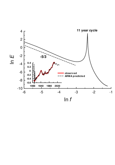
Figure 17: Spectrum of the global temperature anomaly fluctuations in the ln-ln scales for a cutted observed base ARMA model. The straight dashed line is drawn to indicate the Kolmogorov scaling law $E(f)\sim f^{(-5/3)}$.

The author is grateful to J.J. Niemela, to K.R. Sreenivasan, and to SIDC-team, World Data Center for the Sunspot Index, Royal Observatory of Belgium for sharing their data and discussions. The author is also grateful to C.H. Gibson and to R.A. Treumann for their help in improving the paper. A software provided by K. Yoshioka was used at the model computations.

VII Appendix A

The above applied time series decomposition method was developed in the Refs. ks ,bd ,k . In this method a nonstationary mean time series is decomposed into trend, autoregressive and noise components. A random process $X_{t}$ in discrete time $t$ is defined by the following expression:

$$X_{t}=\tau_{t}+\varepsilon_{t}+AR_{t}^{(m)}$$

where $\tau_{t}$ is a trend component, $\varepsilon_{t}$ is an observational noise component, and

$$AR_{t}^{(m)}=\sum_{i=1}^{m}a_{i}X_{t-i}+\eta_{t}^{(1)}$$

is a globally stationary autoregressive (AR) component of order $m$ ($a_{i}$ are the coefficients of a recursive filter, and $\eta_{t}^{(1)}$ is a Gaussian white noise).

A $k$-th order stochastically perturbed difference equation describes evolution of the trend component

$$\Delta^{k}\tau_{t}=\eta_{t}^{(2)}$$

where $\eta_{t}^{(2)}$ is a Gaussian white noise.

In the Ref. k algorithms, using state space modeling and Kalman filter, are suggested for estimation of the model parameters by the maximum likelihood method.

Using so-called autoregressive moving average (ARMA) model one could try to make a prediction. For this model a random process $X_{t}$ in discrete time $t$ is defined by the following expression:

$$X_{t}=\varepsilon_{t}+AR_{t}^{(m)}+\sum_{i=1}^{n}b_{i}\varepsilon_{t-i}$$

where $\varepsilon_{t}$ is Gaussian white noise with zero mean ks ,bd ,k . Again, state space modeling and Kalman filter, are used for estimation of the model parameters by the maximum likelihood method. Figure 14 shows an optimistic prediction produced with this model for a first part of the section IV. Though, continuation of the analogy to the section II makes the scenario much less optimistic. A quasi-Newton method and dynamic restrictions were used for optimization of the model parameters.

We can also play with the model by cutting the observed time series. This procedure reduces relative contribution of the low-frequency fluctuations, presumably of Galactic origin (cf. Fig. 17 and Fig. 15). Then, the insert to the Fig. 17 shows less steep decline of the global temperature anomaly at this (cutted observed base) version of the ARMA model prediction. This game has also another end. One can assume that using a more long time series (observed base), than that we have used in computing the results shown in Fig. 14, one could obtain even more optimistic prediction for the first part of the section IV.

VIII Appendix B

The long-range reconstructions of the sunspot number fluctuations (see, for instance, Refs. sol ,usos1 ) allow us to look on the solar transitional dynamics from a more general point of view. In figure 18 we show a spectrum of such reconstruction for the last 11,000 years (the data, used for computation of the spectrum, is available at usos-recon ). The spectrum was computed using the autoregressive model (with maximum entropy method k ). A semi-logarithmical representation was used in the figure to show an exponential law

$$E(f)\sim e^{-f/f_{e}}$$

The straight line is drawn in Fig. 18 to indicate the exponential law Eq. (B1). Slope of the straight line provides us with the characteristic time scale $T_{e}=1/f_{e}\simeq 176\pm 7$y. The exponential decay of the spectrum excludes the possibility of random behavior and indicates the chaotic behavior of the time series sig ,sun . It is well known that low-order dynamic (deterministic) systems have as a rule exponential decay of $E(f)$ (see, for instance, sun ,o ). As for infinite dimensional dynamic systems with chaotic attractors it is interesting to compare Fig. 18 with figure 3 of the Ref. fa . It should be noted that the 176y period is the third doubling of the period 22y. The 22y period corresponds to the Sun’s magnetic poles polarity switching (see also Appendix C).

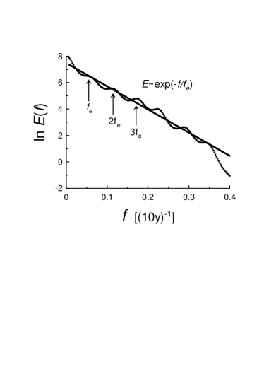
Figure 18: Spectrum of the sunspots number fluctuations in the ln-linear scales (the reconstructed data for the last 11,000 years have been taken from usos-recon ). The straight line is drawn to indicate the exponential law Eq. (B1).

The exponential spectrum can be also produced by a series of Lorentzian pulses with the average width of the individual pulses equals to $\tau$ (though, the distribution of widths of the pulses should be fairly narrow to result in the exponential spectrum).

In Fig. 18 a local maximum corresponding to the frequency $f_{e}$ and its first harmonics have been indicated by arrows. It should be noted that the harmonic $2f_{e}$ corresponds to the well known period $T\simeq 88y$ (see, for instance, Ref. fg ), and the harmonic $3f_{e}$ corresponds to the period $T\simeq 60y$ (cf. section ”A FORECAST”).

IX Appendix C

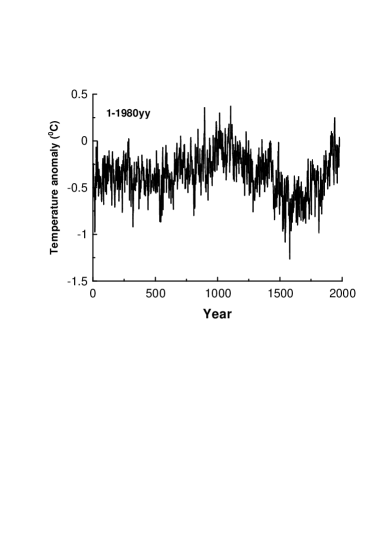
Figure 19: A reconstruction of Northern Hemisphere temperature anomaly for the past 2,000 years (the data was taken from Ref. paleoT ).

It is also useful to consider the above results in content of multicentennial and millennial timescales. Figure 19 shows a reconstruction of Northern Hemisphere temperatures for the past 2,000 years (the data for this figure were taken from Ref. paleoT ). This multi-proxy reconstruction was performed by the authors of Ref. moberg using combination of low-resolution proxies (lake and ocean sediments) with comparatively high-resolution tree-ring data. Figure 20 shows a power spectrum of the data set calculated using the maximum entropy method (as for the spectra shown in Figs. 16 and 18) in the frames of the autoregressive model, because it provides an optimal spectral resolution even for small data sets (see also o ). The spectrum exhibits a rather wide peak indicating a periodic component with a period around 22 y, and a broad-band part with exponential decay. A semilogarithmical plot was used in Fig. 20 (cf Fig. 18) in order to show the exponential decay more clearly (at this plot the exponential decay corresponds to a straight line). Both stochastic and deterministic processes can result in the broad-band part of the spectrum, but the decay in the spectral power is different for the two cases. The exponential decay indicates that the broad-band spectrum for these data arises from a deterministic rather than a stochastic process. Indeed, for a wide class of deterministic systems a broad-band spectrum with exponential decay is a generic feature of their chaotic solutions (see, for instance, Refs. sig ,o ,fa and Appendix B).

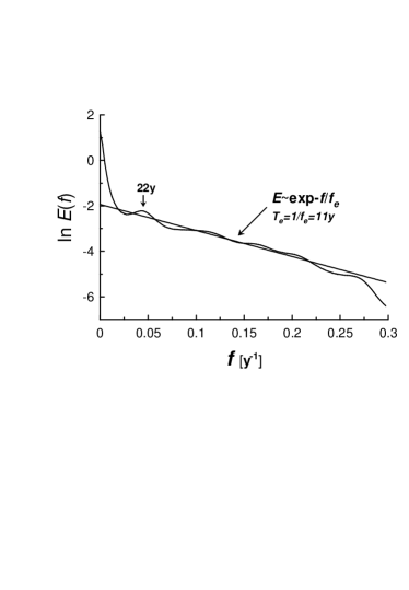
Figure 20: Spectrum of the data, shown in Fig. 19, in semilogarithmical scales. The straight line indicates the exponential decay Eq. (B1).

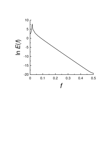
Figure 21: Spectrum of the chaotic fluctuations of the x- component for the Rössler system ($a=0.15$, $b=0.20$, $c=10.0.$)

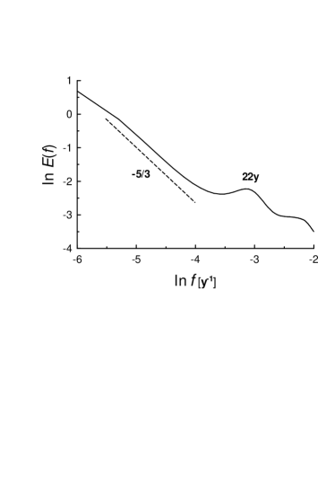
Figure 22: Spectrum of the data, shown in Fig. 19, in ln-ln scales. The dashed straight line indicates the Kolmogorov-like spectrum: $E(f)\sim f^{-5/3}$. The high-frequency part has been cutted in order to show the low-frequency part.

In order to illustrate this and another significant feature of the chaotic power spectra we show in figure 21 a power spectrum for the Rössler system ros

$$\frac{dx}{dt}=-(y+z);~{}~{}\frac{dy}{dt}=x+ay;~{}~{}\frac{dz}{dt}=b+xz-cz$$

chaotic solution, where $a$, $b$ and $c$ are parameters. In this figure one can see a typical picture: a narrow-band peak (corresponding to the fundamental frequency of the system) in a low-frequency part and a broad-band exponential decay in a high-frequency part of the spectrum. Nature of the exponential decay of the power spectra of the chaotic systems is still an unsolved mathematical problem. A progress in solution of this problem has been achieved by the use of the analytical continuation of the equations in the complex domain (see, for instance, fu ,fm ). In this approach the exponential decay of chaotic spectrum is related to a singularity in the plane of complex time, which lies nearest to the real axis. Distance between this singularity and the real axis determines the rate of the exponential decay. If parameters of the dynamical system periodically fluctuate around their mean values, then at certain (critical) intensity of these fluctuations an additional singularity (nearest to the real time axis) can appear. Distance between this singularity and the real axis is determined by period of the periodic fluctuation of the system’s parameters. Therefore, exponential decay rate of the broad-band part of the system spectrum equals the period of the parametric forcing. The chaotic spectrum provides two different characteristic time-scales for the system: a period corresponding to fundamental frequency of the system, $T_{fun}$, and a period corresponding to the exponential decay rate, $T_{e}=1/f_{e}$ (cf Eq. (B1)). The fundamental period $T_{fun}$ can be estimated using position of the low-frequency peak, while the exponential decay rate period $T_{e}=1/f_{e}$ can be estimated using the slope of the straight line of the broad-band part of the spectrum in the semilogarithmical representation (Figs. 20 and 21). From Fig. 20 we obtain $T_{fun}\simeq 22\pm 2$y and $T_{e}\simeq 11\pm 1y$ (the estimated errors are statistical ones). Thus, the solar activity (SSN) period of 11 years is still a dominating factor in the chaotic temperature fluctuations at the millennial time scales , although it is hidden for linear interpretation of the power spectrum (cf Ref. b3 ). In the nonlinear interpretation the additional period $T_{fun}\simeq 22y$ might correspond to the fundamental frequency of the underlying nonlinear dynamical system. It is surprising that this period is close to the 22y period of the Sun’s magnetic poles polarity switching (cf Appendix B). It should be noted that the authors of Ref. mu found a persistent 22y cyclicity in sunspot activity, presumably related to interaction between the 22y period of magnetic poles polarity switching and a relic solar (dipole) magnetic field. Therefore, one cannot rule out a possibility that the broad peak, in a vicinity of frequency corresponding to the 22y period, is a quasi-linear response of the global temperature to the weak periodic modulation by the 22y cyclicity in sunspot activity. I.e. strong enough periodic forcing results in the non-linear (chaotic) response whereas a weak periodic forcing results in a quasi-periodic response.

Finally, figure 22 shows the same power spectrum as in Fig. 20 but in ln-ln scales, where the dashed straight line indicates the Kolmogorov-like behavior: $E(f)\sim f^{-5/3}$, in the lower-frequency part of the spectrum (see section ’A Forecast’ and Fig. 16 for relation between this type of spectrum and galactic turbulence).

References

- (1) S. K. Solanki, I. G. Usoskin, B. Kromer, M. Schüssler and J. Beer, Unusual activity of the Sun during recent decades compared to the previous 11,000 years, Nature, 431, 1084-1087 (2004).
- (2) I.G. Usoskin, S.K. Solanki, M. Schüssler, et al., Millennium-Scale Sunspot Number Reconstruction: Evidence for an Unusually Active Sun since the 1940s, Phys. Rev. Lett. 91, 211101 (2003) (see also arXiv:astro-ph/0310823).
- (3) E.A. Spiegel, and N.O. Weiss, Magnetic activity and variations in solar luminosity, Nature, 287, 616-617 (1980)
- (4) A. Brandenburg, The Case for a Distributed Solar Dynamo Shaped by Near-Surface Shear, ApJ, 625 539-547 (2005) (see also arXiv:astro-ph/0502275).
- (5) H.W. Babcock, The topology of the sun s magnetic field and the 22-year cycle, ApJ. 133 572-589 (1961).
- (6) R.B. Leighton, A Magneto-Kinematic Model of the Solar Cycle, ApJ, 156, 1-26 (1969).
- (7) M. Dikpati, G.de Toma, and P.A. Gilman, Predicting the strength of solar cycle 24 using a flux-transport dynamo-based tool, Geophys. Res. Lett., 33 L05102 (2006).
- (8) A.R. Choudhuri, P. Chatterjee, and J. Jiang, Predicting Solar Cycle 24 With a Solar Dynamo Model, Phys. Rev. Lett. 98, 131101 (2007).
- (9) R.J. Bray, R.E. Loughhead, Sunspots, (Dover Publications, New York, 1979).
- (10) K.R. Sreenivasan and A. Bershadskii, Clustering Properties in Turbulent Signals, J. Stat. Phys., 125, 1141-1153 (2006).
- (11) A. Bershadskii, Transitional dynamics of the solar convection zone, Europhys. Lett., 85, 49002 (2009).
- (12) G. Molchan, private communication.
- (13) M.R. Leadbetter and J.D. Gryer, The variance of the number of zeros of a stationary normal process, Bull. Amer. Math. Soc. 71, 561-563 (1965).
- (14) The data are available at http://sidc.oma.be/sunspot-data/
- (15) R.J. Bray, R.E. Loughead, and C.J Durrant, The solar granulation (Cambridge Univ. Press, Cambridge, 2ed, 1984).
- (16) J.J. Niemela, L. Skrbek, K.R. Sreenivasan, R. J. Donnelly, Turbulent convection at very high Rayleigh numbers, Nature, 404, 837-840 (2000).
- (17) I. G. Usoskin and G. A. Kovaltsov, Cosmic Ray Induced Ionization in the Atmosphere: Full Modeling and Practical Applications, J. Geophys. Res., 111, D21206, (2006).
- (18) N.J. Shaviv, On climate response to changes in the cosmic ray flux and radiative budget, J. Geophys. Res. 110, A08105 (2005).
- (19) J. Kirkby, Cosmic Rays and Climate, Surveys in Geophysics, 28, 333-375 (2007) (see also arXiv:0804.1938).
- (20) The data are available at http://www.cru.uea.ac.uk/cru/ data/temperature/ (N.A. Rayner, et al., Improved analyses of changes and uncertainties in marine temperature measured in situ since the mid-nineteenth century: the HadSST2 dataset, J. Climate, 19, 446-469 (2006)).
- (21) The data are available at http://cdiac.ornl.gov/trends/ co2/lawdome-data.html (D.M. Etheridge, et al., Historical records from the Law Dome DE08, DE08-2, and DSS ice cores).
- (22) The data are available at http://cdiac.ornl.gov/ ftp/trends/co2/maunaloa.co2 (C. D. Keeling, and T.P. Whorf. Atmospheric records from sites in the SIO air sampling network).
- (23) S.M. Tobias and D.W. Hughes, The Influence of Velocity Shear on Magnetic Buoyancy Instability in the Solar Tachocline, ApJ. 603, 785 802 (2004).
- (24) A. Bershadskii, Multiscaling of Galactic Cosmic Ray Flux, Phys. Rev. Lett., 90 041101 (2003) (see also arXiv:astro-ph/0305453).
- (25) M.L. Goldstein, Major Unsolved Problems in Space Plasma Physics, Astrophys. Space Sci. 227, 349 369 (2001).
- (26) The data are available at http://www.srl.caltech.edu/ ACE/ASC/
- (27) P.N. Mayaud, Derivation, Meaning, and Use of Geomagnetic Indices, AGU 1129 Geophys. Monograph 22, (Washington D.C., 1980).
- (28) E. W. Cliver, V. Boriakoff, J. Feynman, Solar Variability and Climate Change: Geomagnetic aa Index and Global Surface Temperature, J. Geophys. Res. Lett. 25, 1035 1038 (1998).
- (29) T. Landscheidt, in ”The solar cycle and terrestrial climate”’, Vazquez, M. and Schmiedere, E, ed., European Space Agency, Special Publication, 463, pp 497-500 (2000).
- (30) The data are available at http://www.ukssdc.ac.uk/ data/wdcc1/wdc menu.html (World Data Centre for Solar-Terrestrial Physics, Chilton).
- (31) C. Fabara and B. Hoeneisen, Global Warming: some back-of-the-envelope calculations, arXiv:physics/0503119 (2005).
- (32) G. Gerlich and R. D. Tscheuschner, Falsification Of The Atmospheric CO2 Greenhouse Effects Within The Frame Of Physics, arXiv:0707.1161 (2007).
- (33) G. Kitagawa, and W. Gersch, Smoothness Priors Analysis of Time Series. (Springer, 1996).
- (34) P.J. Brockwell, and R.A. Davis, Introduction to Time Series and Forecasting. (Springer, 1996).
- (35) G. Kitagawa, Time Series Analysis Programming, Iwanami Shoten. (Tokyo, 1993, in Japanese).
- (36) The data are available at http://www.frontier.iarc. uaf.edu:8080/ igor/research/ice/icedata.php (see also I. Polyakov, et al., Long-Term Ice Variability in Arctic Marginal Seas, Journal of Climate 16, 2078-2085 (2003)).
- (37) N. Scaffeta and B.J. West, Is climate sensitive to solar variability? , Physics Today, 51, 50-51 (2008).
- (38) N. Scaffeta and B.J. West, Estimated solar contribution to the global surface warming using the ACRIM TSI satellite composite, Geophys. Res. Lett., 33, L05708 (2006) (see also arXiv:physics/0509248).
- (39) The data are available at http://www.sec.noaa.gov/ SolarCycle/SC24.
- (40) A.C. Monin and A.M. Yaglom, Statistical Fluid Mechanics (MIT Press, Cambridge, 1975), Vol. 2.
- (41) C.H Gibson, Kolmogorov Similarity Hypotheses for Scalar Fields: Sampling Intermittent Turbulent Mixing in the Ocean and Galaxy, Proc. Roy. Soc. Lond. 434, 149 (1991).
- (42) J. Cho, A. Lazarian, and E.T. Vishniac, Simulations of MHD Turbulence in a Strongly Magnetized Medium, Astrophys. J. 564, 291-301 (2002) (see also arXiv:astro-ph/0205286).
- (43) C.H. Gibson, R.N. Keeler, V.G. Bondur, et al., Submerged turbulence detection with optical satellites, Proc. of SPIE, 6680, 6680-33 (2007) (see also arXiv:0709.0074v2 [astro-ph]).
- (44) The data are available at http://www1.ncdc.noaa.gov/ pub/data/paleo/climate_forcing/solar_variability/usoskin-cosmic-ray.txt (see also I.G. Usoskin, K. Mursula, S.K. Solanki, M. Schuessler, and G.A. Kovaltsov, A physical reconstruction of cosmic ray intensity since 1610. J. Geophys. Res., J. Geophys. Res., 107(A11), 1374-1380 (2002)).
- (45) D.E. Sigeti, Survival of deterministic dynamics in the presence of noise and the exponential decay of power spectrum at high frequencies. Phys. Rev. E, 52, 2443-2457 (1995).
- (46) J. Sun, Y. Zhao, T. Nakamura, and M. Small, From phase space to frequency domain: A time-frequency analysis for chaotic time series, Phys. Rev. E 76, 016220 (2007).
- (47) N. Ohtomo, K. Tokiwano, Y. Tanaka, A. Sumi, S. Terachi, and H. Konno, Exponential Characteristics of Power Spectral Densities Caused by Chaotic Phenomena, J. Phys. Soc. Jpn. 64 1104-1113 (1995).
- (48) J. D. Farmer, Chaotic attractors of an infinite dimensional dynamic system, Physica D, 4, 366-393 (1982).
- (49) J. Feynman, and S.B. Gabriel, Period and phase of the 88-year solar cycle and the Maunder Minimum: Evidence for a chaotic Sun, Solar Physics, 127, 393-403 (1990).
- (50) The data are available at http://www.ncdc.noaa.gov/ paleo/metadata/noaarecon-6267.html
- (51) A. Moberg, D. M. Sonechkin, K. Holmgren, N. M. Datsenko and W. Karl en, Highly variable Northern Hemisphere temperatures reconstructed from low- and high resolution proxy data Nature, 433, 613-617 (2005).
- (52) O.E. Rössler, An equation for continuous chaos, Phys. Lett. A, 35, 397-398 (1976).
- (53) F. Fucito, F. Marchesoni, E. Marianari, G. Parisi, L.Peliti, S. Ruffo, and V. Vulpiani, Approach to equilibrium in a chain of nonlinear oscillators, J. Physique, 43, 707-713 (1982).
- (54) U. Frisch and R. Morf, Intermittency in non-linear dynamics and singularities at complex times, Phys. Rev. 23, 2673 (1981).
- (55) A. Bershadskii, Chaotic dynamics of atmospheric at millennial timescales, arXiv:0903.2795 (2009).
- (56) K. Mursula, I. G. Usoskin, and G. A. Kovaltsov, Persistent 22-year cycle in sunspot activity: Evidence for a relic solar magnetic field, Solar Phys., 198, 51-56, 2001.