On Emergence of Dominating Cliques in Random Graphs

Abstract

Emergence of dominating cliques in Erdös-Rényi random graph model ${{\mathchoice{\hbox{\hbox to0.0pt{\kern 2.1972pt\vrule height=6.35492pt\hss}\hbox{$\displaystyle\rm G$}}}{\hbox{\hbox to0.0pt{\kern 2.1972pt\vrule height=6.35492pt\hss}\hbox{$\textstyle\rm G$}}}{\hbox{\hbox to0.0pt{\kern 1.53804pt\vrule height=4.44846pt\hss}\hbox{$\scriptstyle\rm G$}}}{\hbox{\hbox to0.0pt{\kern 1.0986pt\vrule height=3.17746pt\hss}\hbox{$\scriptscriptstyle\rm G$}}}}(n,p)}$ is investigated in this paper. It is shown this phenomenon possesses a phase transition. Namely, we have argued that, given a constant probability $p$, an $n$-node random graph $G$ from ${{\mathchoice{\hbox{\hbox to0.0pt{\kern 2.1972pt\vrule height=6.35492pt\hss}\hbox{$\displaystyle\rm G$}}}{\hbox{\hbox to0.0pt{\kern 2.1972pt\vrule height=6.35492pt\hss}\hbox{$\textstyle\rm G$}}}{\hbox{\hbox to0.0pt{\kern 1.53804pt\vrule height=4.44846pt\hss}\hbox{$\scriptstyle\rm G$}}}{\hbox{\hbox to0.0pt{\kern 1.0986pt\vrule height=3.17746pt\hss}\hbox{$\scriptscriptstyle\rm G$}}}}(n,p)}$ and for $r=c\log_{1/p}n$ with $1\leq c\leq 2$, it holds: (1) if $p>1/2$ then an $r$-node clique is dominating in $G$ almost surely and, (2) if $p\leq(3-\sqrt{5})/2$ then an $r$-node clique is not dominating in $G$ almost surely. The remaining range of probability $p$ is discussed with more attention. A detailed study shows that this problem is answered by examination of sub-logarithmic growth of $r$ upon $n$.

Keywords: Random graphs, dominating cliques, phase transition.

1 Introduction

The phase transition phenomenon was originally observed as a physical effect. In discrete mathematics, it was originally described by P. Erdös and A. Rényi in [8]. The most frequently property of graphs which have been studied with relation to the phase transitions in random graphs is the connectivity. The recent surveys of known results concerning this area can be find in Refs. [2] and [9], Chapter 5.

Our paper deals with another interesting graph problem that is the emerging of a dominating clique in a random graph. The theory of dominating cliques in random graphs has several nontrivial applications in computer science. The most significant ones are: (1) heuristics in satisfiability search [5] and (2) the construction of a space-efficient interval routing scheme with a small additive stretch for almost all and large-scale distributed systems [13].

1.1 Preliminaries and terminology

Given a graph $G=(V,E)$, a set $S\subseteq V$ is said to be a dominating set of $G$ if each node $v\in V$ is either in $S$ or is adjacent to a node in $S$. The domination number $\gamma(G)$ is the minimum cardinality of a dominating set of $G$.

A clique in $G$ is a maximal set of mutually adjacent nodes of $G$, i.e., it is a maximal complete subgraph of $G$. The clique number, denoted $cl(G)$, is the number of nodes of clique of $G$. If a subgraph $S$ induced by a dominating set is a clique in $G$ then $S$ is called a dominating clique in $G$.

The model of random graphs is introduced in the following way. Let $n$ be a positive integer and let $p\in{\rm I\!R}$, $0\leq p\leq 1$, be a probability of an edge. The (probabilistic) model of random graphs ${\mathchoice{\hbox{\hbox to0.0pt{\kern 2.1972pt\vrule height=6.35492pt\hss}\hbox{$\displaystyle\rm G$}}}{\hbox{\hbox to0.0pt{\kern 2.1972pt\vrule height=6.35492pt\hss}\hbox{$\textstyle\rm G$}}}{\hbox{\hbox to0.0pt{\kern 1.53804pt\vrule height=4.44846pt\hss}\hbox{$\scriptstyle\rm G$}}}{\hbox{\hbox to0.0pt{\kern 1.0986pt\vrule height=3.17746pt\hss}\hbox{$\scriptscriptstyle\rm G$}}}}(n,p)$ consists of all graphs with $n$-node set $V=\{1,\dots,n\}$ such that each graph has at most ${n\choose 2}$ edges being inserted independently with probability $p$. Consequently, if $G$ is a graph with node set $V$ and it has $|E(G)|$ edges, then a probability measure $\Pr$ defined on ${\mathchoice{\hbox{\hbox to0.0pt{\kern 2.1972pt\vrule height=6.35492pt\hss}\hbox{$\displaystyle\rm G$}}}{\hbox{\hbox to0.0pt{\kern 2.1972pt\vrule height=6.35492pt\hss}\hbox{$\textstyle\rm G$}}}{\hbox{\hbox to0.0pt{\kern 1.53804pt\vrule height=4.44846pt\hss}\hbox{$\scriptstyle\rm G$}}}{\hbox{\hbox to0.0pt{\kern 1.0986pt\vrule height=3.17746pt\hss}\hbox{$\scriptscriptstyle\rm G$}}}}(n,p)$ is given by:

$$\Pr[G]=p^{|E(G)|}(1-p)^{{n\choose 2}-|E(G)|}~{}.$$

This model is also called Erdös-Rényi random graph model [2, 9].

Let $A$ be any set of graphs from ${\mathchoice{\hbox{\hbox to0.0pt{\kern 2.1972pt\vrule height=6.35492pt\hss}\hbox{$\displaystyle\rm G$}}}{\hbox{\hbox to0.0pt{\kern 2.1972pt\vrule height=6.35492pt\hss}\hbox{$\textstyle\rm G$}}}{\hbox{\hbox to0.0pt{\kern 1.53804pt\vrule height=4.44846pt\hss}\hbox{$\scriptstyle\rm G$}}}{\hbox{\hbox to0.0pt{\kern 1.0986pt\vrule height=3.17746pt\hss}\hbox{$\scriptscriptstyle\rm G$}}}}(n,p)$ with a property $Q$. We say that almost all graphs have the property $Q$ iff:

$$\Pr[A]\to 1\quad\emph{as}\quad n\to\infty~{}.$$

The term ”almost surely” stands for ”with the probability approaching $1$ as $n\to\infty$”.

1.2 Previous work and our result

Dominating sets and cliques are basic structures in graphs and they have been investigated very intensively. To determine whether the domination number of a graph is at most $r$ is an NP-complete problem [6]. The maximum-clique problem is one of the first shown to be NP-hard [11]. A well-known result of B. Bollobás, P. Erdös et al. states that the clique number in random graphs ${\mathchoice{\hbox{\hbox to0.0pt{\kern 2.1972pt\vrule height=6.35492pt\hss}\hbox{$\displaystyle\rm G$}}}{\hbox{\hbox to0.0pt{\kern 2.1972pt\vrule height=6.35492pt\hss}\hbox{$\textstyle\rm G$}}}{\hbox{\hbox to0.0pt{\kern 1.53804pt\vrule height=4.44846pt\hss}\hbox{$\scriptstyle\rm G$}}}{\hbox{\hbox to0.0pt{\kern 1.0986pt\vrule height=3.17746pt\hss}\hbox{$\scriptscriptstyle\rm G$}}}}(n,p)$ is bounded by a very tight bounds [2, 3, 10, 12, 15, 16]. Let $b=1/p$ and let

$$r_{0}=\log_{b}n-2\log_{b}\log_{b}n+\log_{b}2+\log_{b}\log_{b}e~{},$$ (1)

$$r_{1}=2\log_{b}n-2\log_{b}\log_{b}n+2\log_{b}e+1-2\log_{b}2~{}.$$ (2)

J. G. Kalbfleisch and D. W. Matula [10, 12] proved that a random graph from ${\mathchoice{\hbox{\hbox to0.0pt{\kern 2.1972pt\vrule height=6.35492pt\hss}\hbox{$\displaystyle\rm G$}}}{\hbox{\hbox to0.0pt{\kern 2.1972pt\vrule height=6.35492pt\hss}\hbox{$\textstyle\rm G$}}}{\hbox{\hbox to0.0pt{\kern 1.53804pt\vrule height=4.44846pt\hss}\hbox{$\scriptstyle\rm G$}}}{\hbox{\hbox to0.0pt{\kern 1.0986pt\vrule height=3.17746pt\hss}\hbox{$\scriptscriptstyle\rm G$}}}}(n,p)$ does not contain cliques of the order greater than $\lceil r_{1}\rceil$ and less or equal than $\lfloor r_{0}\rfloor$ almost surely. (See also [3, 15, 16].) The domination number of a random graph have been studied by B. Wieland and A. P. Godbole in [17].

The phase transition of dominating clique problem in random graphs was studied independently by M. Nehéz and D. Olejár in [13, 14] and J. C. Culberson, Y. Gao, C. Anton in [5]. It was shown in [5] that the property of having a dominating clique is monotone, it has a phase transition and the corresponding threshold probability is $p^{*}=(3-\sqrt{5})/2$. The standard first and the second moment methods (based on the Markov’s and the Chebyshev’s inequalities, respectively, see [1, 9]) were used to prove this result. However, the preliminary result of M. Nehéz and D. Olejár [14] pointed out that to complete the behavior of random graphs in all spectra of $p$ needs a more accurate analysis, namely in the case when $(3-\sqrt{5})/2<p\leq 1/2$. The main result of this paper is the refinement of the previous results from [5, 13, 14]. Let us formulate this as the following theorem.

Theorem 1

Let $0<p<1$ be fixed and let ${\rm I\!L}x$ denote $\log_{1/(1-p)}x$. Let $r$ be order of a clique such that $\lfloor r_{0}\rfloor\leq r\leq\lceil r_{1}\rceil$. Let $\delta(n):{{\rm I\!N}}\to{{\rm I\!N}}$ be an arbitrary slowly increasing function such that $\delta(n)=o(\log n)$ and let $G\in{{\mathchoice{\hbox{\hbox to0.0pt{\kern 2.1972pt\vrule height=6.35492pt\hss}\hbox{$\displaystyle\rm G$}}}{\hbox{\hbox to0.0pt{\kern 2.1972pt\vrule height=6.35492pt\hss}\hbox{$\textstyle\rm G$}}}{\hbox{\hbox to0.0pt{\kern 1.53804pt\vrule height=4.44846pt\hss}\hbox{$\scriptstyle\rm G$}}}{\hbox{\hbox to0.0pt{\kern 1.0986pt\vrule height=3.17746pt\hss}\hbox{$\scriptscriptstyle\rm G$}}}}(n,p)}$ be a random graph. Then:

1. If $p>1/2$, then an $r$-node clique is dominating in $G$ almost surely;

2. If $p\leq(3-\sqrt{5})/2$, then an $r$-node clique is not dominating in $G$ almost surely;

3. If $(3-\sqrt{5})/2<p\leq 1/2$, then an $r$-node clique:

   • is dominating in $G$ almost surely, if $r\geq{{\rm I\!L}n}+\delta(n)$,

   • is not dominating in $G$ almost surely, if $r\leq{{\rm I\!L}n}-\delta(n)$,

   • is dominating with a finite probability $f(p)$ for a suitable function $f:[0,1]\to[0,1]$, if $r={{\rm I\!L}n}+O(1)$.

To prove Theorem 1 the first and the second moment method were used. The leading part of our analysis follows from a property of a function defined as a ratio of two random variables which count dominating cliques and all cliques in random graphs, respectively. The critical values of $p$: $(3-\sqrt{5})/2$ and $1/2$, respectively, are obtained from the bounds (1), (2) see [10, 12].

The rest of this paper contains the proof of the Theorem 1. Section 2 contains the preliminary results. An expected number of dominating cliques in ${{\mathchoice{\hbox{\hbox to0.0pt{\kern 2.1972pt\vrule height=6.35492pt\hss}\hbox{$\displaystyle\rm G$}}}{\hbox{\hbox to0.0pt{\kern 2.1972pt\vrule height=6.35492pt\hss}\hbox{$\textstyle\rm G$}}}{\hbox{\hbox to0.0pt{\kern 1.53804pt\vrule height=4.44846pt\hss}\hbox{$\scriptstyle\rm G$}}}{\hbox{\hbox to0.0pt{\kern 1.0986pt\vrule height=3.17746pt\hss}\hbox{$\scriptscriptstyle\rm G$}}}}}(n,p)$ is estimated here. The main result is proved in section 3. Possible applications are discussed in section 4.

2 Preliminary results

For $r>1$, let $S$ be an $r$-node subset of an $n$-node graph $G$. Let $A$ denote the event that ”$S$ is a dominating clique of $G\in{{\mathchoice{\hbox{\hbox to0.0pt{\kern 2.1972pt\vrule height=6.35492pt\hss}\hbox{$\displaystyle\rm G$}}}{\hbox{\hbox to0.0pt{\kern 2.1972pt\vrule height=6.35492pt\hss}\hbox{$\textstyle\rm G$}}}{\hbox{\hbox to0.0pt{\kern 1.53804pt\vrule height=4.44846pt\hss}\hbox{$\scriptstyle\rm G$}}}{\hbox{\hbox to0.0pt{\kern 1.0986pt\vrule height=3.17746pt\hss}\hbox{$\scriptscriptstyle\rm G$}}}}}(n,p)$”. Let $in_{r}$ be the associated $0$-$1$ (indicator) random variable on ${\mathchoice{\hbox{\hbox to0.0pt{\kern 2.1972pt\vrule height=6.35492pt\hss}\hbox{$\displaystyle\rm G$}}}{\hbox{\hbox to0.0pt{\kern 2.1972pt\vrule height=6.35492pt\hss}\hbox{$\textstyle\rm G$}}}{\hbox{\hbox to0.0pt{\kern 1.53804pt\vrule height=4.44846pt\hss}\hbox{$\scriptstyle\rm G$}}}{\hbox{\hbox to0.0pt{\kern 1.0986pt\vrule height=3.17746pt\hss}\hbox{$\scriptscriptstyle\rm G$}}}}(n,p)$ defined as follows: $in_{r}=1$ if $G$ contains a dominating clique $S$ and $in_{r}=0$, otherwise. Let $X_{r}$ be a random variable that denotes the number of $r$-node dominating cliques. More precisely, $X_{r}=\sum in_{r}$ where the summation ranges over all sets $S$. The following lemma expresses the expectation of $X_{r}$.

Lemma 1

[13] The expectation $E(X_{r})$ of the random variable $X_{r}$ is given by:

$$E(X_{r})={n\choose r}p^{{r\choose 2}}(1-p^{r}-(1-p)^{r})^{n-r}~{}.$$ (3)

We use the following properties adopted from [15], pp. 501–502.

Claim 1. Let $0<p<1$ and $k\leq(\eta-1)\frac{\ln n}{\ln p}$, $\eta<0$ starting with some positive integer $n$. Then:

$$(1-p^{k})^{n}=\exp(-np^{k})\left(1+O(np^{2k})\right)=1-np^{k}+O\left(np^{2k}\right)~{}.$$

Claim 2. Let $k=o(\sqrt{n})$, then:

$$n^{\underline{k}}=n(n-1)\cdots(n-k+1)=n^{k}\left(1-{k\choose 2}\frac{1}{n}+O\left(\frac{k^{4}}{n^{2}}\right)\right)~{}.$$

The upper bound on $r$ in ${\mathchoice{\hbox{\hbox to0.0pt{\kern 2.1972pt\vrule height=6.35492pt\hss}\hbox{$\displaystyle\rm G$}}}{\hbox{\hbox to0.0pt{\kern 2.1972pt\vrule height=6.35492pt\hss}\hbox{$\textstyle\rm G$}}}{\hbox{\hbox to0.0pt{\kern 1.53804pt\vrule height=4.44846pt\hss}\hbox{$\scriptstyle\rm G$}}}{\hbox{\hbox to0.0pt{\kern 1.0986pt\vrule height=3.17746pt\hss}\hbox{$\scriptscriptstyle\rm G$}}}}(n,p)$ is stated in the following lemma.

Lemma 2

Let $b=1/p$ and

$$r_{u}=2\log_{b}n-2\log_{b}\log_{b}n+2\log_{b}e+1-2\log_{b}2~{}.$$ (4)

A random graph from ${\mathchoice{\hbox{\hbox to0.0pt{\kern 2.1972pt\vrule height=6.35492pt\hss}\hbox{$\displaystyle\rm G$}}}{\hbox{\hbox to0.0pt{\kern 2.1972pt\vrule height=6.35492pt\hss}\hbox{$\textstyle\rm G$}}}{\hbox{\hbox to0.0pt{\kern 1.53804pt\vrule height=4.44846pt\hss}\hbox{$\scriptstyle\rm G$}}}{\hbox{\hbox to0.0pt{\kern 1.0986pt\vrule height=3.17746pt\hss}\hbox{$\scriptscriptstyle\rm G$}}}}(n,p)$ does not contain dominating cliques of the order greater than $r_{u}$ with probability approaching $1$ as $n\to\infty$.

Remark 1

Note that the upper bounds $r_{u}$ and $r_{1}$ are the same. The argument for estimation of $r_{1}$ is the same as in Lemma 2.

To obtain conditions for an existence of dominating cliques in random graphs it is sufficient to estimate the variance $Var(X_{r})$. We can use the fact that the clique number in random graphs lyes down in a tight interval. We use the bounds (1) and (2) due to [10, 12]. The estimation of the variance $Var(X_{r})$ is stated in the following lemma.

Lemma 3

Let p be fixed, $0<p<1$ and $\lfloor r_{0}\rfloor\leq r\leq\lceil r_{1}\rceil$. Let

$$\beta=\min\{~{}2/3,~{}-2\log_{b}(1-p)~{}\}~{}.$$

Then:

$$Var(X_{r})=E(X_{r})^{2}\cdot O\left(\frac{(\log n)^{3}}{n^{\beta}}\right)~{}.$$ (5)

The following claim expresses the number of the dominating cliques in random graphs.

Lemma 4

Let $p$, $r$ and $\beta$ be as before, and

$$X_{r}={n\choose r}p^{{r\choose 2}}(1-p^{r}-(1-p)^{r})^{n-r}\times\left\{1+O\left(\frac{(\log n)^{3}}{n^{\beta/2}}\right)\right\}~{}.$$ (6)

The probability that a random graph from ${\mathchoice{\hbox{\hbox to0.0pt{\kern 2.1972pt\vrule height=6.35492pt\hss}\hbox{$\displaystyle\rm G$}}}{\hbox{\hbox to0.0pt{\kern 2.1972pt\vrule height=6.35492pt\hss}\hbox{$\textstyle\rm G$}}}{\hbox{\hbox to0.0pt{\kern 1.53804pt\vrule height=4.44846pt\hss}\hbox{$\scriptstyle\rm G$}}}{\hbox{\hbox to0.0pt{\kern 1.0986pt\vrule height=3.17746pt\hss}\hbox{$\scriptscriptstyle\rm G$}}}}(n,p)$ contains $X_{r}$ dominating cliques with $r$ nodes is $1-O\left((\log n)^{-3}\right)$.

3 Proof of Theorem 1

For $r>1$, let $Y_{r}$ be the random variable on ${\mathchoice{\hbox{\hbox to0.0pt{\kern 2.1972pt\vrule height=6.35492pt\hss}\hbox{$\displaystyle\rm G$}}}{\hbox{\hbox to0.0pt{\kern 2.1972pt\vrule height=6.35492pt\hss}\hbox{$\textstyle\rm G$}}}{\hbox{\hbox to0.0pt{\kern 1.53804pt\vrule height=4.44846pt\hss}\hbox{$\scriptstyle\rm G$}}}{\hbox{\hbox to0.0pt{\kern 1.0986pt\vrule height=3.17746pt\hss}\hbox{$\scriptscriptstyle\rm G$}}}}(n,p)$ which denotes the number of $r$-node cliques. According to [15],

$$Y_{r}={n\choose r}p^{{r\choose 2}}(1-p^{r})^{n-r}\times\left\{1+O\left(\frac{(\log n)^{3}}{\sqrt{n}}\right)\right\}~{}.$$ (7)

The ratio $X_{r}/Y_{r}$ expresses the relative number of dominating cliques (with $r$ nodes) to all cliques (with $r$ nodes) in ${{\mathchoice{\hbox{\hbox to0.0pt{\kern 2.1972pt\vrule height=6.35492pt\hss}\hbox{$\displaystyle\rm G$}}}{\hbox{\hbox to0.0pt{\kern 2.1972pt\vrule height=6.35492pt\hss}\hbox{$\textstyle\rm G$}}}{\hbox{\hbox to0.0pt{\kern 1.53804pt\vrule height=4.44846pt\hss}\hbox{$\scriptstyle\rm G$}}}{\hbox{\hbox to0.0pt{\kern 1.0986pt\vrule height=3.17746pt\hss}\hbox{$\scriptscriptstyle\rm G$}}}}(n,p)}$ and it attains a value in the interval [0, 1]. By analysis of the asymptotic of $X_{r}/Y_{r}$ as $n$ tends $\infty$ we obtain our main result.

Let us examine the limit value of the ratio $X_{r}/Y_{r}$:

$$\frac{X_{r}}{Y_{r}}=\left(\frac{1-p^{r}-(1-p)^{r}}{1-p^{r}}\right)^{n-r}\times$$

$$\times\left\{1+O\left(\frac{(\log n)^{3}}{\sqrt{n}}\right)\right\}\times\left\{1+O\left(\frac{(\log n)^{3}}{n^{\beta/2}}\right)\right\}~{}.$$ (8)

The most important term of the expression (8) is the first one, since the last two terms tend to $1$ as $n\to\infty$. Let us define $\alpha:[0,1]\to{\rm I\!R}$ by:

$$\alpha(p)=-\log_{1/p}(1-p)~{}.$$

The plot of its graph is in fig. 1 and for the simplification, we will write also $\alpha$ instead of $\alpha(p)$. Note that

$$(1-p)^{r}=p^{r\alpha}~{}.$$ (9)

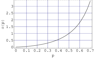
Figure 1: The graph of the function $\alpha(p)=-\log_{1/p}(1-p)$.

According to Claim 1 and (9) we have:

$$\left(\frac{1-p^{r}-(1-p)^{r}}{1-p^{r}}\right)^{n-r}=\left(1-\frac{p^{r\alpha}}{1-p^{r}}\right)^{n-r}=$$

$$=\exp\left(\frac{-np^{r\alpha}}{1-p^{r}}\right)\cdot\left\{1+O\left(np^{2r\alpha}\right)\cdot\left[1+O\left(\frac{(\log n)^{2+\alpha}}{n}\right)\right]\right\}=$$

$$=\exp\left(\frac{-np^{r\alpha}}{1-p^{r}}\right)\cdot\left[1+O\left(np^{2r\alpha}\right)\right]~{}.$$

Let us analyze the asymptotic behavior of the ratio $X_{r}/Y_{r}$ as $n$ tends to $\infty$. According to the assumption $n\to\infty$, we can write $X_{r}/Y_{r}$ in the following two equivalent forms:

$$\frac{X_{r}}{Y_{r}}=\exp\left(-\frac{np^{r\alpha}}{1-p^{r}}\right)~{},$$

or, applying (11), as:

$$\frac{X_{r}}{Y_{r}}=\exp\left(-\frac{n(1-p)^{r}}{1-p^{r}}\right)~{}.$$

Using bounds (1) and (2), the admissible number of nodes of a clique $r$ depends on $n$ as (we consider the leading term only):

$$r=\rho\log_{b}n,$$ (10)

where $1\leq\rho\leq 2$. This results in:

$$\frac{X_{r}}{Y_{r}}=\exp\left(-\frac{n^{1-\rho\alpha}}{1-p^{r}}\right),$$

and one has three different cases:

1. $1-\rho\alpha<0,\ \forall\ \rho\in[1,2]$  $\Leftrightarrow$  $p>\frac{1}{2}$ ,

2. $1-\rho\alpha\geq 0,\ \forall\ \rho\in[1,2]$  $\Leftrightarrow$  $p\leq\frac{3-\sqrt{5}}{2}$ ,

3. $1-\rho\alpha$ changes sign as $\rho$ varies in $[1,2]$  $\Leftrightarrow$  $\frac{3-\sqrt{5}}{2}<p\leq\frac{1}{2}$ .

The first case implies

$$\lim_{n\to\infty}\frac{X_{r}}{Y_{r}}=1,$$

that means the $r-$node cliques is dominating in $G$ almost surely. The second case implies

$$\lim_{n\to\infty}\frac{X_{r}}{Y_{r}}=0,$$

and therefore a $r-$node clique is not dominating in $G$ almost surely. In the third case, there exists a value of $\rho$ (for each $p$) in the interval $[1,2]$:

$$\hat{\rho}=\frac{1}{\alpha(p)},$$

for which we have:

$$r=\hat{\rho}\log_{b}n=\log_{1/(1-p)}n$$

and

$$\lim_{n\to\infty}\frac{X_{r}}{Y_{r}}=\exp\left(-n(1-p)^{r}\right)=e^{-1}.$$

The ratio $X_{r}/Y_{r}$ approaches $1$ ($0$) for $\rho>\hat{\rho}$ ($\rho<\hat{\rho}$). Due to corrections of order less than $\Theta(\log n)$ to the equation (10) taken with $\rho=\hat{\rho}$ the value of $e^{-1}$ to be changed to another constant greater or equal than $0$ and less or equal than $1$. The details are given here. Let $\delta(n):{{\rm I\!N}}\to{{\rm I\!N}}$ be an increasing function such that $\delta(n)=o(\log n)$.

If $r=\hat{\rho}\log_{b}n+\delta(n)$, then $X_{r}/Y_{r}$ approaches $1$ as  $\exp\left(-(1-p)^{\delta(n)}\right)$.

If $r=\hat{\rho}\log_{b}n-\delta(n)$, then $X_{r}/Y_{r}$ approaches $0$ as  $\exp\left(-(1-p)^{-\delta(n)}\right)$.

And finally, if $r$ differs from $\hat{\rho}\log_{b}n$ by a constant $\lambda$, then the ratio $X_{r}/Y_{r}$ asymptotically looks like  $\exp(-(1-p)^{\lambda})$.
The proof is complete.  $\diamondsuit$

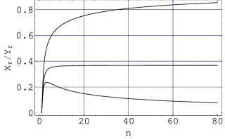
Figure 2: The plot of the fraction $X_{r}/Y_{r}$ versus $n$ for three different choices of $\rho$ in the intermediate case when $\frac{3-\sqrt{5}}{2}<p\leq\frac{1}{2}$. In all three cases $p$ is set to be $0.45$ and $\rho$ varies (from the top to the bottom) as: $\rho=1.9$, $\rho=1/\alpha(0.45)$, and finally $\rho=1.05$.

4 Discussion

We have claimed the conditions for the existence of dominating cliques in Erdös-Rényi random graph model. Our result is the refinement of the previous ones from [5, 13, 14].

For possible applications of this result we address the two works of J. C. Culberson, Y. Gao, C. Anton [5] and M. Nehéz and D. Olejár [13]. The paper [5] deals with heuristics in satisfiability search. For the second application, described in [13], we mention the construction of a space-efficient interval routing scheme with a small additive stretch in almost all networks modelled by random graphs ${\mathchoice{\hbox{\hbox to0.0pt{\kern 2.1972pt\vrule height=6.35492pt\hss}\hbox{$\displaystyle\rm G$}}}{\hbox{\hbox to0.0pt{\kern 2.1972pt\vrule height=6.35492pt\hss}\hbox{$\textstyle\rm G$}}}{\hbox{\hbox to0.0pt{\kern 1.53804pt\vrule height=4.44846pt\hss}\hbox{$\scriptstyle\rm G$}}}{\hbox{\hbox to0.0pt{\kern 1.0986pt\vrule height=3.17746pt\hss}\hbox{$\scriptscriptstyle\rm G$}}}}(n,p)$ where $p>1/2$. An application of this result can be found in decentralized content sharing systems based on the peer-to-peer (shortly P2P) paradigm such as Freenet which uses the idea of interval routing for retrieving files from local datastores according to keys [4].

Acknowledgement. This work has been supported by Gratex Research, Bratislava, by CU grant No. 403/2007 and by the VEGA grant No. 1/3042/06.

Appendix

Proof of Lemma 2.

The proof follows from the Markov’s inequality [9], p. 8:

$$\Pr[~{}X\geq t~{}]\leq\frac{E(X)}{t}~{},\qquad t>0~{}.$$

Let us denote $\alpha=\log_{1/p}\left(\frac{1}{1-p}\right)=-\log_{b}(1-p)$. Note that:

$$(1-p)^{r}=p^{r\alpha}~{}.$$ (11)

Let $r=(2-\varepsilon)\log_{b}n$, where $0\leq\varepsilon<1$. According to Claim 1 we have three cases: $p>1/2,\ p=1/2$ and $p<1/2$. The first two of them can be analyzed together, performing elementary computations we obtain:

$$(1-p^{r}-(1-p)^{r})^{n-r}\approx 1-n^{\epsilon-1}\to^{n\to\infty}1,~{}~{}\emph{if}\quad p\geq\frac{1}{2}.$$

In the case $p<1/2$ the same kind of algebra shows that

$$(1-p^{r}-(1-p)^{r})^{n-r}\approx\exp\left[-n^{1-\frac{(2-\epsilon)\ln(1-p)}{\ln(p)}}\right],~{}~{}\emph{if}\quad p<\frac{1}{2}.$$

We distinguish two different asymptotics in the previous formula. For given $p<1/2$ they are separated by the condition

$$1-(2-\hat{\epsilon})\frac{\ln(1-p)}{\ln(p)}=0.$$

This is solved with respect to $\hat{\epsilon}$ as:

$$\hat{\epsilon}=2-\frac{\ln(p)}{\ln(1-p)}.$$

Now we have:

• for $\epsilon>\hat{\epsilon}$

  $$(1-p^{r}-(1-p)^{r})^{n-r}\to 0\quad\mbox{as}\quad n\to\infty,$$

• for $\epsilon<\hat{\epsilon}$

  $$(1-p^{r}-(1-p)^{r})^{n-r}\to 1\quad\mbox{as}\quad n\to\infty,$$

With respect to upper and lower bound on size of a dominating clique we require $\epsilon$ ranges between $0$ and $1$. This requirement defines then two critical values of the probability $p$:

• $\hat{\epsilon}=1$ - in this case

  $$p=\frac{1}{2},$$

• $\hat{\epsilon}=0$ - in this case

  $$p=\frac{3-\sqrt{5}}{2}.$$

The Stirling’s formula (e.g. [16], p. 127) yields to:

$${n\choose r}p^{{r\choose 2}}\sim\left(\frac{nep^{(r-1)/2}}{r}\right)^{r}~{}.$$ (12)

Consequently,

$${n\choose r_{u}}p^{{r_{u}\choose 2}}\to 1\qquad\emph{and}\qquad{n\choose r_{u}+1}p^{{r_{u}+1\choose 2}}\sim\frac{\log_{b}n}{n}\to 0$$

The rest follows from the Markov’s inequality (Appendix) for $t=1$.  $\diamondsuit$

Proof of Lemma 3.

In order to prove this lemma we will estimate the variance of $X_{r}$:

$$Var(X_{r})=E(X^{2}_{r})-E^{2}(X_{r})~{}.$$ (13)

The expectation of $X^{2}_{r}$ can be expressed in the following way:

$$E(X^{2}_{r})=\sum_{j=0}^{r}{n\choose r}{r\choose j}{n-r\choose r-j}\cdot{p^{2}}^{{r\choose 2}-{j\choose 2}}\times$$

$$\times(1-p^{r}-(1-p)^{r})^{2n-4r+2j}\cdot\Pr[S_{r}^{1},S_{r}^{2}]~{}.$$ (14)

The equation (14) follows from the next analysis. The nodes of the first dominating clique $S_{r}^{1}$ can be chosen in ${n\choose r}$ ways. The dominating cliques $S_{r}^{1}$, $S_{r}^{2}$ can (but need not to) have $j$ common nodes. These nodes can be chosen in ${r\choose j}$ ways. The remaining $(r-1)$ nodes of the second dominating clique $S_{r}^{2}$ have to be chosen from $(n-r)$ nodes of $V(G)\setminus V(S_{r}^{1})$. Now we shall choose edges: both dominating cliques are $r$-node complete graphs and therefore they contain $2{r\choose 2}$ edges. But $S_{r}^{1}$, $S_{r}^{2}$ can have a nonempty intersection - a complete $j$-node subgraph. Therefore ${j\choose 2}$ edges were counted twice. Both subgraphs $S_{r}^{1}$, $S_{r}^{2}$ are dominating cliques and so all $n-2r+j$ nodes of the set $V(G)\setminus[V(S_{r}^{1})\cup V(S_{r}^{2})]$ are ”good” with respect to both $S_{r}^{1}$, $S_{r}^{2}$. The last term, $\Pr[S_{r}^{1},S_{r}^{2}]$ denotes the probability that the nodes of $V(S_{r}^{1})\setminus V(S_{r}^{2})$ are good with respect to $S_{r}^{2}$ and the nodes of $V(S_{r}^{2})\setminus V(S_{r}^{1})$ are good with respect to $S_{r}^{1}$. It is sufficient to estimate $\Pr[S_{r}^{1},S_{r}^{2}]$ by 1.

To prove that $Var(X_{r})$ is asymptotically less than $E^{2}(X_{r})$, we extract the expression $E^{2}(X_{r})$ in front of the sum stated by the equation (14). We have:

$$E(X_{r}^{2})\leq E^{2}(X_{r})\cdot\sum_{j=0}^{r}{n\choose r}^{-1}{r\choose j}{n-r\choose r-j}\cdot p^{-{j\choose 2}}\cdot Q(p,r,j)~{},$$ (15)

where $Q(p,r,j)=(1-p^{r}-(1-p)^{r})^{-2r+2j}$.

First we estimate the expression $Q(p,r,j)$. Let us denote $\alpha=-\log_{b}(1-p)$, as before. Recall that  $(1-p)^{r}=p^{r\alpha}$. Let us also denote:

$$\nu=\min\{1,-\log_{b}(1-p)\}~{}.$$ (16)

Therefore, from $\lfloor r_{0}\rfloor\leq r\leq\lceil r_{1}\rceil$ (cf. [15]), Claim 1 and (11), it follows:

$$Q(p,r,j)<\left[1-p^{r_{0}}-p^{\alpha r_{0}}\right]^{-2r}\leq$$

$$\leq\left[1-\frac{(\log_{b}n)^{2}}{2n\cdot\log_{b}e}-\left(\frac{(\log_{b}n)^{2}}{2n\cdot\log_{b}e}\right)^{\alpha}\right]^{-4\log_{b}n}=$$

$$=\exp\left\{4\log_{b}n\cdot\left[\frac{(\log_{b}n)^{2}}{2n\cdot\log_{b}e}+\left(\frac{(\log_{b}n)^{2}}{2n\cdot\log_{b}e}\right)^{\alpha}\right]\right\}\times$$

$$\times\left(1+O\left(\frac{\left(\log n\right)^{1+2\nu}}{n^{2\nu}}\right)\right)=$$

$$=\exp\left(\frac{2(\log_{b}n)^{3}}{n\cdot\log_{b}e}\right)\cdot\exp\left(\frac{4(\log_{b}n)^{2\alpha+1}}{(2n\cdot\log_{b}e)^{\alpha}}\right)\cdot\left(1+O\left(\frac{(\log n)^{1+2\nu}}{n^{2\nu}}\right)\right),$$

where $\nu=\min\{1,\alpha\}$. Since

$$\frac{2(\log_{b}n)^{3}}{n\cdot\log_{b}e}\to 0\qquad\emph{and}\qquad\frac{4(\log_{b}n)^{2\alpha+1}}{(2n\cdot\log_{b}e)^{\alpha}}\to 0$$

as $n\to\infty$, the value of $Q(p,r,j)$ is $1+o(1)$ or, more precisely:

$$Q(p,r,j)=1+O\left(\frac{(\log n)^{2\nu+1}}{n^{2\nu}}\right)~{}.$$ (17)

Now we can concentrate our effort on the estimation of the sum

$$\sum_{j=0}^{r}{n\choose r}^{-1}{r\choose j}{n-r\choose r-j}\cdot p^{-{j\choose 2}}~{},$$ (18)

where:

$$\lfloor r_{0}\rfloor\leq r\leq\lceil r_{1}\rceil~{}.$$

We use a similar approach as D. Olejár and E. Toman in [15], pp. 504–506. This sum was also estimated in Subsection 5.3. of [16] (pp. 77–80), but we need more accurate calculation here. First we introduce the following notation:

$$S(n,r,c,d)=\sum_{j=c}^{d}{n\choose r}^{-1}{r\choose j}{n-r\choose r-j}\cdot b^{{j\choose 2}}~{}.$$

Our solution is based on the idea to divide the sum $S(n,r,a,b)$ into three parts by the following way:

$$S(n,r,0,r)\leq S(n,r,0,1)+S(n,r,2,r_{2})+S(n,r,r_{2},r)~{},$$ (19)

where:

$$r_{2}=(1+\lambda)\log_{b}n\qquad\emph{for}\qquad 0<\lambda<1~{}.$$

All these three parts will be estimated separately. Using Claim 2, the first part is estimated as follows:

$$S(n,r,0,1)={n-r\choose r}{n\choose r}^{-1}+r\cdot{n-r\choose r-1}{n\choose r}^{-1}=$$

$$=\left(1-\frac{r^{2}}{n}\right)\left[1+O\left(\frac{(\log n)^{4}}{n^{2}}\right)\right]+\frac{r^{2}}{n}+O\left(\frac{(\log n)^{3}}{n^{2}}\right)=$$

$$=1+O\left(\frac{(\log n)^{4}}{n^{2}}\right)~{}.$$ (20)

To estimate the second part, it is sufficient to analyze the binomial coefficients. (See also [16], pp. 79–80.)

$${n\choose r}^{-1}{r\choose j}{n-r\choose r-j}=\frac{r!}{n^{\underline{r}}}\cdot\frac{r^{\underline{j}}}{j!}\cdot\frac{(n-r)^{\underline{r-j}}}{(r-j)!}=$$

$$=\frac{r^{\underline{j}}\cdot(r-j)!}{(r-j)!}\cdot\frac{r^{\underline{j}}}{j!}\cdot\frac{(n-r)^{\underline{r-j}}}{n^{\underline{j}}\cdot(n-j)^{\underline{r-j}}}\ \leq\ \frac{r^{\underline{j}}\cdot r^{\underline{j}}}{j!\cdot n^{\underline{j}}}\ \leq\ \frac{r^{2j}}{j!\cdot n^{\underline{j}}}\ \sim\ \frac{r^{2j}}{j!\cdot n^{j}}$$

We use the Stirling’s formula in the following form:

$$j!~{}\sim~{}\left(\frac{j}{e}\right)^{j}~{}.$$

Consequently,

$${n\choose r}^{-1}{r\choose j}{n-r\choose r-j}\cdot b^{{j\choose 2}}\ \sim\ \left(\frac{r^{2}\cdot b^{j/2}\cdot e}{j\cdot n\cdot\sqrt{b}}\right)^{j}~{}.$$ (21)

The members of the sum $S(n,r,2,r_{2})$ attain their asymptotic maximum for $j=r_{2}$. More precisely, letting $j=r_{2}=(1+\lambda)\log_{b}n$  we have:

$$\frac{r^{2}\cdot b^{j/2}\cdot e}{j\cdot n\cdot\sqrt{b}}=O\left(\frac{\log n}{n^{1/2-\lambda/2}}\right)~{}.$$

Thus,

$$S(n,r,2,r_{2})\leq\left(\frac{c_{1}\cdot\log n}{n^{1/2-\lambda/2}}\right)^{2}+\left(\frac{c_{1}\cdot\log n}{n^{1/2-\lambda/2}}\right)^{3}+\dots+\left(\frac{c_{1}\cdot\log n}{n^{1/2-\lambda/2}}\right)^{r_{2}}~{}$$

for a suitable constant $c_{1}$. It yields:

$$S(n,r,2,r_{2})=O\left(\frac{(\log n)^{2}}{n^{1-\lambda}}\right)~{}.$$ (22)

To estimate the sum $S(n,r,r_{2},r)$ we extract the term ${n\choose r}^{-1}\cdot b^{{r\choose 2}}$:

$$S(n,r,r_{2},r)={n\choose r}^{-1}\cdot b^{{r\choose 2}}\cdot\sum_{j=r_{2}}^{r}{r\choose r-j}{n-r\choose r-j}\cdot p^{{r\choose 2}-{j\choose 2}}~{}.$$

To obtain the upper bound on the right-hand side sum, we substitute $\lceil r_{1}\rceil$ for $r$ in its upper border and $\lceil r_{1}\rceil+1$ for $r$ in all the summands. The reasoning of such a substitution is the assertion of Lemma 2 and Remark 1. We have:

$$S(n,r,r_{2},r)\leq{n\choose r}^{-1}\cdot b^{{r\choose 2}}\cdot\sum_{j=r_{2}}^{\lceil r_{1}\rceil}{\lceil r_{1}\rceil+1\choose\lceil r_{1}\rceil+1-j}{n-\lceil r_{1}\rceil-1\choose\lceil r_{1}\rceil+1-j}\cdot p^{{\lceil r_{1}\rceil+1\choose 2}-{j\choose 2}}~{}.$$

Let us put $k=\lceil r_{1}\rceil+1-j$. Consequently,

$$S(n,r,r_{2},r)\leq$$ (23)

$$\leq{n\choose r}^{-1}\cdot b^{{r\choose 2}}\cdot\sum_{k=1}^{\lceil r_{1}\rceil-r_{2}+1}{\lceil r_{1}\rceil+1\choose k}{n-\lceil r_{1}\rceil-1\choose k}\cdot p^{k[\lceil r_{1}\rceil-(k-1)/2]}~{}.$$

Note that

$${\lceil r_{1}\rceil+1\choose k}{n-\lceil r_{1}\rceil-1\choose k}\cdot p^{k[\lceil r_{1}\rceil-(k-1)/2]}\leq\left((\lceil r_{1}\rceil+1)\cdot np^{\lceil r_{1}\rceil-(k-1)/2}\right)^{k},$$

and

$$\lceil r_{1}\rceil-(k-1)/2\geq\lceil r_{1}\rceil/2+r_{2}/2=$$

$$=(3/2+\lambda/2)\log_{b}n-\log_{b}\log_{b}n+O(1)~{}.$$

It yields:

$$(\lceil r_{1}\rceil+1)\cdot np^{\lceil r_{1}\rceil-(k-1)/2}=O\left(\frac{(\log n)^{2}}{n^{1/2+\lambda/2}}\right)~{}.$$ (24)

According to (23) and (24),

$$S(n,r,r_{2},r)\leq{n\choose r}^{-1}\cdot b^{{r\choose 2}}\cdot O\left(\frac{(\log n)^{2}}{n^{1/2+\lambda/2}}\right)~{}.$$

The term ${n\choose r}^{-1}\cdot b^{{r\choose 2}}$ can be estimated using the Stirling’s formula. The estimation is the same as in the proof of Lemma 2, see (12). Thus,

$${n\choose r_{1}}^{-1}b^{{r_{1}\choose 2}}\to 1~{},$$

$${n\choose r}^{-1}b^{{r\choose 2}}\sim\frac{(\log_{b}n)^{c}}{n^{c}}\to 1~{},$$

if $r=\lceil r_{1}\rceil-c$, where $c\geq 1$. Hence,

$$S(n,r,r_{2},r)=O\left(\frac{(\log n)^{2}}{n^{1/2+\lambda/2}}\right)~{}.$$ (25)

Let us summarize our results:

• Eq. (20) shows that $S(n,r,0,1)$ is close to $1$ uniformly with respect to $\lambda$.

• Eq. (22) shows that the ”mid” term $S(n,r,2,r_{2})$ of the sum-splitting (19) is close to zero however, non-uniformly in $\lambda$. As $\lambda$ approaches $1$ from the left (i.e. the node number approaches its upper bound) $S(n,r,2,r_{2})$ decreases to zero slowly.

• Eq. (25) shows that $S(n,r,r_{2},r)$ is close to zero uniformly in $\lambda$. (We choose $\lambda=0$ as the uniform upper bound.)

Thus, we have:

$$E(X^{2}_{r})=E^{2}(X_{r})\cdot\left[1+O\left(\frac{(\log n)^{2}}{n^{2/3}}\right)\right]\cdot\left[1+O\left(\frac{\left(\log n\right)^{2\nu+1}}{n^{2\nu}}\right)\right]$$

$$=E^{2}(X_{r})\cdot\left[1+O\left(\frac{\left(\log n\right)^{3}}{n^{\beta}}\right)\right]~{},$$

where  $\nu=\min\{~{}1,-\log_{b}(1-p)~{}\}$  and
$\beta=\min\{~{}2/3,~{}-2\log_{b}(1-p)~{}\}$ .

Substituting into (13) we obtain the estimation of $Var(X_{r})$.  $\diamondsuit$

Proof of Lemma 4.

It follows from the Chebyshev’s inequality [9]: if $Var(X)$ exists, then:

$$\Pr[|X-E(X)|\geq t]\geq\frac{Var(X)}{t^{2}}~{},\qquad t>0~{}.$$

Letting $t=E(X_{r})\cdot(\log n)^{3}\cdot n^{-\beta/2}$ and using Lemma 3, we obtain the assertion of Lemma 4.  $\diamondsuit$

References

[1]
N. Alon, J. Spencer: The probabilistic method (2nd
edition), John Wiley & Sons, New York, 2000.
[2]
B. Bollobás: Random Graphs (2nd edition), Cambridge
Studies in Advanced Mathmatics 73, 2001.
[3]
B. Bollobás, P. Erdös: Cliques in random graphs,
Math. Proc. Cam. Phil. Soc. (1976), 80, pp. 419–427.
[4]
L. Bononi: A Perspective on P2P Paradigm and Services,
Slide courtesy of A. Montresor, URL: http://www.cs.unibo.it/people/faculty/bononi//AdI2004/AdI11.pdf
[5]
J. C. Culberson, Y. Gao, C. Anton: Phase Transitions of
Dominating Clique Problem and Their Implications to Heuristics in
Satisfiability Search, In Proc. 19th Int. Joint Conf. on
Artificial Intelligence, IJCAI 2005, 78–83.
[6]
M. R. Garey, D.S. Johnson: Computers and Intractability,
Freeman, New York, 1979.
[7]
J. L. Gross, J. Yellen: Handbook of Graph Theory, CRC
Press, 2003.
[8]
P. Erdös, A. Rényi: On the evolution of random graphs,
Publ. Math. Inst. Hungar. Acad. Sci., 5 (1960), pp. 17–61.
[9]
S. Janson, T. Luczak, A. Rucinski: Random Graphs, John
Wiley & Sons, New York, 2000.
[10]
J. G. Kalbfleisch: Complete subgraphs of random hypergraphs
and bipartite graphs, In Proc. 3rd Southeastern Conf. of
Combinatorics, Graph Theory and Computing, Florida Atlantic
University, 1972, pp. 297–304.
[11]
R. M. Karp: Reducibility among combinatorial problems, In
Complexity of Computer Computation, (R. E. Miller and J. W.
Thatcher, eds.), Plenum Press, 1972, 24, pp. 85–103.
[12]
D. W. Matula: The largest clique size in a random graph,
Technical report CS 7608, Dept. of Comp. Sci. Southern Methodist
University, Dallas, 1976.
[13]
M. Nehéz, D. Olejár: An Improved Interval Routing Scheme
for Almost All Networks Based on Dominating Cliques, In Proc.
16th Int. Symposium on Algorithms and Computation, ISAAC 2005,
Springer Berlin-Heidelberg, LNCS 3827/2005, 524–532.
[14]
M. Nehéz, D. Olejár: On Dominating Cliques in Random
Graphs, Research Report, KAM-Dimatia Series 2005-750, Charles
University, Prague, 2005.
[15]
D. Olejár, E. Toman: On the Order and the Number of
Cliques in a Random Graph, Math. Slovaca, 47(5), 1997, pp.
499–510.
[16]
E. M. Palmer: Graphical Evolution, John Wiley & Sons,
Inc., New York, 1985.
[17]
B. Wieland, A. P. Godbole: On the Domination Number of a
Random Graph, Electronic Journal of Combinatorics, 8(1), #R37,
2001.