A Novel Approach to Study Highly Correlated Nanostructures:
The Logarithmic Discretization Embedded Cluster Approximation

Abstract

This work proposes a new approach to study transport properties of highly correlated local structures. The method, dubbed the Logarithmic Discretization Embedded Cluster Approximation (LDECA), consists of diagonalizing a finite cluster containing the many-body terms of the Hamiltonian and embedding it into the rest of the system, combined with Wilson’s idea of a logarithmic discretization of the representation of the Hamiltonian. The physics associated with both one embedded dot and a double-dot side-coupled to leads is discussed in detail. In the former case, the results perfectly agree with Bethe ansatz data, while in the latter, the physics obtained is framed in the conceptual background of a two-stage Kondo problem. A many-body formalism provides a solid theoretical foundation to the method. We argue that LDECA is well suited to study complicated problems such as transport through molecules or quantum dot structures with complex ground states.

I Introduction

The study of nanostructures has been motivated, on the one hand, by the potential applications in molecular electronics devices molecular or in quantum computing qcomp and, on the other hand, by the search for a more profound understanding of fundamental many-body physics such as the Kondo effect. Experimentally, not only the existence of the Kondo effect in quantum dots GG or single-molecule transistors molecules has been established, but it has also been demonstrated that nanostructures can be designed to produce more exotic phases such as multi-channel physics and thus, non-Fermi liquid behavior.nonfermi On the theoretical side, while the single-impurity case is well understood by means of firmly established analytical bethe and numerical methods, such as the Numerical Renormalization Group technique (NRG),Wilson the search for unconventional effects, non-equilibrium behavior, and the need to model complex real structures, such as molecules or multi-dot geometries, has triggered the development of alternative methods.tDMRG ; fRG ; ferrari99 ; davidovich02 ; anda02 ; chiappe03 For instance, the procedure of exactly diagonalizing a finite cluster containing the many-body terms and embedding it into the rest of the system, the Embedded Cluster Approximation (ECA), has satisfactorily been used to study transport in nanoscopic structures in the last few years.ferrari99 ; davidovich02 ; anda02 ; chiappe03 Ideas similar to the embedded cluster method have been applied to the metal-insulator transition of the Hubbard model.busser2 ; chiappe99 ; Tremblay

Incorporating ideas from the Density Matrix Renormalization Group method (DMRG) white into NRG and vice versa has also resulted in substantial improvements in, e.g., the calculation of dynamical properties hofstetter or time-evolution schemes, anders which now allows one to address problems previously out of reach for either method. In the same spirit, it is the objective of this paper to present the Logarithmic Discretization Embedded Cluster Approximation (LDECA) approach to study highly correlated electrons in nano-scale systems, combining ECA with Wilson’s idea of a logarithmic discretization of the conduction band.Wilson As one of our main results, we utilize many-body arguments to provide a solid theoretical justification of this formalism. Although the ECA method, due to the embedding process, is designed to analyze the infinite system, it produces results that depend on the cluster’s size, which, in some cases, has led to controversial results. busser04 ; hm08 LDECA not only successfully reduces these finite-size effects, but, more importantly, it also optimizes the description of the system in the vicinity of the Fermi level, allowing for the analysis of lower energy scales than accessible to ECA.

To demonstrate the potential of the method, we focus on the physics of the Kondo effect in a single-dot, where we find excellent agreement with exact Bethe ansatz (BA) results. As there is a timely interest in more involved versions of Kondo physics, such as multi-channel situations, nonfermi SU(4),su4 ; ecasu4 as well as two-stage Kondo (TSK) effects,wiel ; two-stage ; Grempel ; pedro ; zitko06 ; zitko07 we further apply LDECA to study a double-dot structure side-connected to leads. This system, with a subtle TSK ground state similar to the one studied in Ref. Grempel, , is an important testbed for our approach. Our results are encouraging, and we thus envision the successful future application of LDECA to more involved systems such as molecules adsorbed at metallic surfaces molecules ; quique or dot structures with subtle ground states.nonfermi

The plan of the paper is as follows. We first provide a discussion of the theoretical foundation of the method in terms of diagrammatic perturbation theory in Sec. II. For the sake of a clear presentation, we choose to provide a pedagogical account of the theory, therefore the details will be given in an appendix (App. A). Our results for the two systems, one embedded dot and a two dot model, are covered in Secs. III and Sec. IV, respectively. For both models, we discuss the local density of states and the conductance as a function of gate potential. We close with a summary in Sec. V.

II The “Logarithmic Discretization Embedded Cluster Approximation” (LDECA)

Figure 1: (Color online) (a) Schematic description of the steps needed in the implementation of the ECA and LDECA methods for the particular case of one quantum dot coupled to a conduction band. The system is separated into two parts: the first one contains the many-body terms and the first few neighboring sites in the lead. This forms the cluster to be exactly diagonalized, with $L=N+1$ sites. The second part is the rest of the lead, a semi-infinite tight-binding chain. A crucial step, which allows the simulation of Kondo physics, is the embedding of the cluster into the remaining part of the system. This step is performed through a Dyson equation, which amounts to a summation of an infinite family of Feynman diagrams arising from perturbation theory. (b) Diagrammatic expansion associated to the Dyson equation. The dressed propagators (in green, darkly shaded), which reestablish the artificially broken connection between sites N and R (through a hopping term $V$), are calculated as a function of the bare propagators (gray, lightly shaded). Note that the equation for the dressed propagator N+1,j does not have an independent bare term, since the bare propagator N+1,j is zero.

Similarly to the ECA method, LDECA is supposed to treat localized impurity systems that consist of a region with many-body interactions weakly coupled to non-interacting conduction bands. The approach is based on the idea that the many-body effects of the impurities are local in character. With this in mind, we proceed in three steps: first, out of the complete system, one isolates a cluster with $L$ sites that consists of the impurities plus their $N$ nearest neighboring sites in the tight-binding lattice (thus, $L=N+1$, in the case of a single impurity). In this cluster is where most of the many-body effects are expected to be confined. In a second step the cluster’s Green function is computed with exact diagonalization, which then, in a last step, is embedded into the rest of the tight-binding lattice.ferrari99 ; davidovich02 ; anda02 ; chiappe03 ; ecasu4 ; busser04 ; martins05 ; interference ; otras1 ; otras2 ; Armando The precise meaning of the embedding step is described below.

The theoretical foundation of the method is outlined using the Anderson single-impurity Hamiltonian describing a dot connected to a semi-infinite lead. Hewsonbook The total Hamiltonian reads

$$H_{T} = V_{g}\sum_{\sigma}n_{0\sigma}+H_{MB}+$$ (1)

$$t^{\prime}\sum_{\sigma}(c_{0\sigma}^{\dagger}c_{1\sigma}+c_{1\sigma}^{\dagger}c_{0\sigma})+H_{\mbox{\small band}},$$

where

$$H_{MB} = U/2\sum_{\sigma}n_{0\sigma}n_{0\bar{\sigma}},$$ (2)

and

$$H_{\mbox{\small band}} = \sum_{i=1\sigma}^{\infty}t_{i}(c_{i\sigma}^{\dagger}c_{i+1\sigma}+c_{i+1\sigma}^{\dagger}c_{i\sigma})\,.$$ (3)

The first two terms of $H_{T}$ represent the impurity, which has a diagonal energy, the gate potential $V_{g}$, and a Coulomb repulsion $U$ in the Hamiltonian $H_{MB}$. The third term is the hybridization of the impurity with the band and finally, $H_{\mbox{\small band}}$ represents the continuous spectrum, in this case modeled by a semi-infinite non-interacting chain. $c_{i\sigma}^{\dagger}$ is a fermion creation operator acting on site $i$, with a spin index $\sigma=\uparrow\downarrow$. $n_{i\sigma}=c_{i\sigma}^{\dagger}c_{i\sigma}$ is the particle density operator. $t^{\prime}$ and $t_{i}$ are the hopping matrix elements between the dot and the leads and in the leads, respectively. A tight-binding band with a semi-elliptical density of states is obtained with the choice of $t_{i}=1$.

This problem can be treated within the framework of quantum perturbation theory. The standard many-body perturbation theory formulation generally considers the kinetic energy as the unperturbed Hamiltonian and the many-body terms as the perturbation. This permits the use of Wick’s theorem to formulate a diagrammatic expansion for the propagators of the system. In our case, however, we adopt an opposite point of view. The unperturbed Hamiltonian consists of two parts, the isolated cluster, which includes the impurity and its neighborhood, and the rest of the system, as represented by the two dashed boxes in Fig. 1 (a). The kinetic energy associated to the connection of these two subsystems is now considered to be the perturbation. This seems to be an appropriate starting point to describe a system where the many-body interactions are local, so that the cluster may contain most of the relevant physics we wish to describe. However, one faces several difficulties in a theory of this kind. The most important one is the fact that, in this case, Wick’s theorem is not valid and, as a consequence, it cannot be used to develop the diagrammatic expansion. However, perturbation theory provides us with a way of proposing a locator-propagator diagrammatic expansion and establishing a criterion to sum up the most important families of diagrams (for details, see Appendix A).

Therefore, following the strategy outlined above, the unperturbed Hamiltonian $H_{0}$ is given by:

$$H_{0} = H_{\mbox{\small cluster}}+H_{\mbox{\small rest}}$$ (4)

where

$$H_{\mbox{\small cluster}} = V_{g}\sum_{\sigma}n_{0\sigma}+H_{MB}+$$ (6)

$$t^{\prime}\sum_{\sigma}c_{0\sigma}^{\dagger}c_{1\sigma}+\sum_{i=1\sigma}^{N}t_{i}c_{i\sigma}^{\dagger}c_{i+1\sigma}+\mbox{h.c.},$$

and

$$H_{\mbox{\small rest}} = \sum_{i=N+1\sigma}^{\infty}t_{i}(c_{i\sigma}^{\dagger}c_{i+1\sigma}+\mbox{h.c.})\,.$$ (7)

Figure 1(a) schematically represents the two parts of the system. Note that one of the internal connections of the lead, represented by a red line, labeled with a $V=t_{N}$ in the figure, is artificially broken by this procedure and the two parts of the unperturbed Hamiltonian, $H_{\mbox{\small cluster}}$ and $H_{\mbox{\small rest}}$, can be solved exactly. The ground state of $H_{\mbox{\small cluster}}$ with $N$ sites of the lead plus the impurity is obtained by using the Lanczos method.Elbio In addition, using a continued fraction scheme, the cluster Green functions at zero temperature are then evaluated. The Green functions for $H_{\mbox{\small rest}}$ are calculated exactly since it constitutes a one-body problem.

To restore the artificially broken connection between sites $N$ and $N+1$, the interaction between the cluster and the rest of the lead,

$$H_{\mbox{\small p}} = V\sum_{\sigma}c_{N\sigma}^{\dagger}c_{N+1\sigma}+\mbox{h.c.},$$ (8)

is taken as the perturbation in the many-body diagrammatic expansion for the Green functions. This step represents the embedding of the cluster into the rest of the system.

For the sake of clarity, we restrict the discussion to the local diagonal Green function at the impurity site, while it is straightforward to calculate a non-diagonal Green function at two arbitrary sites $i$ and $j$ following the same prescriptions. To obtain the causal Green functions we follow the standard framework of an expansion in terms of Feynman diagrams.Abrikosov The causal Green function for the impurity site can be obtained from

$$G_{00,\sigma}(t-t^{\prime})=\frac{\left\langle{\mathcal{T}}\{c_{0\sigma}(t)c^{\dagger}_{0\sigma}(t^{\prime})S(\infty)\}\right\rangle_{0}}{\left\langle S(\infty)\right\rangle_{0}}\,,$$ (9)

where, as usual, $S(\infty)$ is the evolution operator and $\mathcal{T}$ is the time order operator. The mean values are calculated in the ground state of the unperturbed Hamiltonian $H_{0}$.

The evolution operator $S(\infty)$ is expanded in increasing orders of $H_{\mbox{\small p}}$, which, when replaced in Eq. (9), gives rise to a perturbation series for the Green function.

The Green function of the system at the impurity, as discussed in the appendix, can be written using a general Dyson equation, as schematically shown in Fig. 1(b):

$$G_{00,\sigma}(\omega)=G^{(0)}_{00,\sigma}(\omega)+\sum_{i}G^{(0)}_{0i,\sigma}(\omega)\Sigma^{\sigma}_{i}(\omega)G_{i0,\sigma}(\omega)$$ (10)

where $i$ is restricted to be either $0$ or $N$, $\omega$ denotes frequency, and the self-energy $\Sigma^{\sigma}_{i}(\omega)$ is defined as

$$\Sigma^{\sigma}_{i}(\omega)=\Sigma^{\sigma}_{N}(\omega)\delta_{iN}+\Sigma^{\sigma}_{0}(\omega)\delta_{i0}.$$ (11)

While $\Sigma^{\sigma}_{N}(\omega)$ is a simple self-energy, $\Sigma^{\sigma}_{0}(\omega)$ represents an infinite expansion (see Eq. (LABEL:eq18a) in the Appendix). It can only be calculated approximately, although this can be done in a systematic way by including terms in the expansion up to a certain order in $U$. Diagrams with a similar topological structure appear in the calculation of the one particle Green function for the Hubbard or Anderson impurity Hamiltonians treated in the thermodynamic limit.qual In addition, in Ref. Tremblay, , a diagrammatic expansion for an interacting lattice in the strong coupling limit was used in order to include effects of long-range interactions beyond the exact diagonalization of a finite cluster.

The key approximation of LDECA is guided by a comparison of the two contributions to the self-energy given in Eq. (11). While $\Sigma^{\sigma}_{0}$ strongly depends on the size of the cluster through the non-diagonal Green function $[G^{(0)}_{0N,\sigma}(\omega)]^{2}$, $\Sigma^{\sigma}_{N}$ does not. This fact can be of great help in establishing a hierarchy between these two contributions to the self-energy. In order to achieve this, the applicability of this expansion is restricted to the vicinity of the Fermi energy, where we know the physics of the Kondo regime is contained. Following Wilson’s logarithmic discretization of the lead’s density of states,Wilson the Hamiltonian is rewritten by adopting hopping elements that depend on the site index $i$:

$$t_{i}=\frac{(1+\lambda^{-1})}{2\lambda^{(i-1)/2}}~{}t$$ (12)

where $\lambda>1$ is a constant, $i\geq 1$ ($i=0$ being the position of the impurity), and we take $t=1$ as the unit of energy. Note that in the limit of $\lambda\to 1$, the above expression for $t_{i}$ describes a semi-elliptical band, rather than the flat band commonly used in standard NRG calculations; however, close to the Fermi energy the two bands have the same low-energy physics. It is worth noting here that the above discussion applies to both ECA and LDECA, with the exception that in ECA $\lambda$ is taken to be 1, implying that the band is not discretized.

The implications of this logarithmic discretization with respect to the contribution of the Hilbert space states are twofold: (i) near the dot, states of all energies are taken into account; (ii) of the states far from the dot, only those near the Fermi level are considered, while high energy ones are neglected. hewson2 Although by this procedure high energy scales are not well treated, it permits to accurately describe much smaller energy scales than it is possible with $\lambda=1$, for the same cluster size. This procedure is justified if the physics of the problem depends only on states with energy close to the Fermi level, as it is the case in the Kondo effect, discussed in this paper.

As discussed in the appendix, around Eq. (42), from Eqs. (34) and (LABEL:eq18a) one realizes that $\Sigma^{\sigma}_{N}\sim\lambda^{-(N-1)}$ and $\Sigma^{\sigma}_{0}\sim f(N)~{}\lambda^{-(N-1)N/2}$, such that

$$\frac{\Sigma^{\sigma}_{0}(\omega)}{\Sigma^{\sigma}_{N}(\omega)}\sim f(N)\,\lambda^{-(N-1)(N/2-1)}\,.$$ (13)

The function $f(N)$ is an intricate function of N which goes asymptotically to zero as N increases above the Kondo cloud length $\xi_{K}$, wich has a magnitude inversely proportional to the Kondo temperatureAffleck . This is the reason why even for $\lambda=1$ (ECA), the self energy $\Sigma^{\sigma}_{0}$ will eventually become negligible in the limit of $N\gg\xi_{K}$ and can be disregarded for sufficiently large N. However, this is a length scale typically much larger than the value for which, according to Eq. (13), the self energy $\Sigma^{\sigma}_{0}$ can be neglected in comparison to $\Sigma^{\sigma}_{N}$. Taking $\lambda=\sqrt{2}$, for example, for a cluster with $N=9$, we get $\Sigma^{\sigma}_{0}/\Sigma^{\sigma}_{N}\sim 10^{-5}$, reflecting the fact that, for a cluster size which permits diagonalization with a relatively modest numerical effort, the contribution to the self-energy can be reduced to $\Sigma^{\sigma}_{N}$. This is a very favorable situation because $\Sigma^{\sigma}_{0}$ is a very complex object (see Appendix) that can be obtained only approximately, while $\Sigma^{\sigma}_{N}$ is very simple and can be calculated exactly. Therefore, here lies the key reason to introduce the logarithmic discretization into the procedure.

Within this approximation, i.e., neglecting $\Sigma^{\sigma}_{0}$, the embedding is carried out using Eq. (34) and therefore, Eq. (10) can be simplified to

$$G_{00\sigma}(\omega)=G^{(0)}_{00\sigma}(\omega)+G^{(0)}_{0N\sigma}V^{2}g_{N+1,\sigma}(\omega)G_{N0,\sigma}(\omega)\,.$$ (14)

Note that the Green function of the semi-infinite linear chain at the site N+1, $g_{N+1,\sigma}(\omega)$, representing the leads, depends on the value of the parameter $\lambda$. For $\lambda=1$, it is the Green function, $g^{sc}$, of a uniform semi-linear chain, given by $g^{sc}(\omega)=(\omega\pm\sqrt{\omega^{2}-4t^{2}})/(2t^{2})$.

Before presenting results obtained with LDECA in the next two sections, we want to discuss some general aspects of the embedding procedure. If we were to study the low energy excitations by diagonalizing an undressed cluster without performing the embedding, the necessity of incorporating a large amount of states lying in the Kondo peak region would require the diagonalization of a cluster of $N$ sites such that $\lambda^{-N/2}t\lesssim T_{\rm k}$, i.e., the energy scale associated with the broken link $V$ in Fig. 1(a) would have to be less than the Kondo temperature. In order to fulfill this condition, and at the same time choose a value of $\lambda$ that still adequately describes the neighborhood of the Fermi energy, the value of $N$ would have to be such that the Lanczos diagonalization would become impractical due to the size of the Hilbert space. The embedding process solves this problem in a simple way by rendering the numerical diagonalization of a small cluster compatible with a correct description of the energy region immediately around the Fermi by allowing the contribution $\Sigma^{\sigma}_{0}(\omega)$ to the self-energy to be disregarded. This approximation, even for $\lambda=1$, has shown to be surprisingly reliable to reproduce the Kondo regime properties of various systems, showing sufficiently fast convergence with cluster size.otras2 ; Busser1

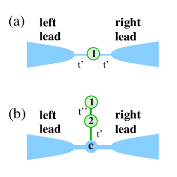
Figure 2: (Color online) Sketch of the quantum dot geometries studied in this work. (a) Single quantum dot connected to two leads. (b) Two side-connected quantum dots studied in Sec. IV.

III Results: LDECA and 1QD

In this section, LDECA is applied to study the conductance and the local density of states (LDOS) of a single quantum dot connected to two leads [see Fig.2(a)]. This case allows for a comparison of our results with an exact solution obtained from BA.bethe Applying a standard basis transformation onto symmetric and anti-symmetric combinations of states (at sites located symmetrically with respect to the dot) the two-leads Hamiltonian can be effectively written as having only one lead, rendering it identical to Eq. (1). This shows that this example constitutes a one-channel Kondo problem.conduc

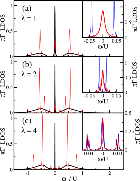
Figure 3: (Color online) (a)-(c): Local density of states for $\lambda=1,2$ and $4$, respectively, and a cluster size $L=8$. Thin (red) lines represent the LDOS as obtained directly from the LDECA procedure (ECA in the case of the top panel), while thick (black) lines are the LDOS for the same parameters, but after the broadening of the resonances using (Eq. 15) has been applied, as explained in Sec.III.1. In the insets, we show a comparison of the LDOS of the bare cluster (thin (blue) line) and after embedding (thick (red) line) for small values of $\omega$. All calculations done for $U=1.0$ and $U/\pi\Gamma=6.3$.

III.1 The local density of states

We start with a discussion of the effect of the $\lambda$-discretization on the LDOS. We expect that a larger density of poles close to the Fermi energy $E_{\rm F}$ is induced by the discretization, while fewer poles will be present away from $E_{\rm F}$. The first aspect, the accumulation of poles close to $E_{\rm F}$ is advantageous to properly describe Kondo physics. To still obtain a reasonable approximation to the LDOS away from the $E_{\rm F}$, it turns out that it is preferable to use a $\omega$-dependent broadening scheme, and we first detail this technical aspect.

The dressed LDOS at the impurity is a collection of poles located at $\omega_{p}$, each one with its own weight $W_{p}$, given by the non-linear Dyson equation used in LDECA. As a consequence of the LDOS normalization, the weights satisfy $\sum_{p}W_{p}=2$. In order to avoid distorting the LDOS curve through the artificially large separation of the poles away from the Fermi energy caused by the logarithmic discretization, and following methods employed in NRG,bulla ; Hewsonbook we write the LDOS as a sum of logarithmic Gaussians,bulla

$$\rho(\omega)=\sum_{p}~{}~{}\frac{{\mbox{e}}^{-b^{2}/4}}{b~{}W_{p}~{}\sqrt{\pi}}~{}{\mbox{exp}}\left(\frac{(\ln{\omega}-\ln{W_{p}})^{2}}{b^{2}}\right)$$ (15)

where $b$ is an arbitrary number that defines, together with $W_{p}$, the width of a pole located at $\omega_{p}$. We choose logarithmic Gaussians to represent the delta functions rather than the usual Gaussians or Lorentzians because this function is asymmetric with respect to $\omega_{p}$. This asymmetry, which effectively shifts the spectral weight of each pole to higher energies, compensates for the accumulation of poles at low energies in relation to higher energies, caused by the logarithmic discretization.bulla As pointed out in Ref. Hewsonbook, , this procedure results in high-energy peaks that are slightly broader and asymmetric than in the case of the true LDOS.

In Fig. 3, we show the LDOS at the impurity for the particle-hole symmetric situation $V_{\rm g}=-U/2$ and different values of $\lambda$ (thin red line) calculated with LDECA with a cluster of $L=8$ sites. An imaginary part $\eta=0.001$, common to all poles, was used for all curves that are obtained with a plain Lorentzian broadening of delta-functions (thin (red) lines in the main panels). The thick black lines show the LDOS using the logarithmic Gaussian broadening with $b=0.5$. In this case, we obtain the characteristic LDOS for the Kondo problem, consisting of a three-peak structure, with two of them located at $\omega=V_{\rm g}$ and $\omega=V_{\rm g}+U$ and the third one, the Kondo resonance, located at the Fermi level $E_{\rm F}=0$. The notable difference between the LDOS for $\lambda=1$ and $\lambda>1$ is the sizeable narrowing of the Kondo peak, in qualitative agreement with NRG Hewsonbook (compare panels (a) with panels (b) and (c) in Fig. 3). A more quantitative comparison with, e.g., NRG, will be presented elsewhere. We wish to draw the reader’s attention to the inset of each panel, showing a comparison of the undressed LDOS [thin (blue) line] with the dressed LDOS [thick (red) line]. One can clearly see that the LDOS for the ‘bare’ cluster (before embedding) vanishes at the Fermi energy, while the LDOS after embedding is finite at $\omega=0$, corroborating the notion that the embedding step is crucial to capture Kondo physics.

Figure 4(a) shows the LDOS for several values of the hybridization parameter $\Gamma$ at the particle-hole symmetric point, and Fig. 4(b) for a fixed ratio of $U/\pi\Gamma=3.5$ and several values of the gate potential. We define the hybridization as $\Gamma=\pi\rho_{0}t^{\prime 2}$, where $\rho_{0}$ is the band density of states at the Fermi level. The top panel illustrates how the width of the Kondo resonance, i.e., $T_{\rm K}$, decreases when $\Gamma$ is reduced. In the bottom panel, we see how the LDOS for a fixed $U/\pi\Gamma=3.5$ changes as the gate potential $V_{\rm g}$ is varied. Note that the Kondo resonance is pinned at $E_{\rm F}$. In contrast, for $|V_{\rm g}|>U$ [dashed (green) curve, for $V_{\rm g}/U=-1.7$] the quantum dot is doubly occupied and therefore there is no Kondo effect. In such a case, the LDOS has just one broad peak located at $\omega=V_{\rm g}+U$.

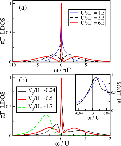
Figure 4: (Color online) (a) Local density of states for the particle-hole symmetric gate potential $V_{g}=-U/2$ for $U=1.0$, $\lambda=2$, and different values of $U/\pi\Gamma$, going from the Kondo regime ($U/\pi\Gamma=6.3$) to the intermediate valence regime ($U/\pi\Gamma=1.5$). (b) LDOS for three different values of the gate potential for $U/\pi\Gamma=3.5$ and $\lambda=2$. The inset shows a comparison of results for $V_{g}/U=-0.24$ between $\lambda=2$ [solid (black) curve, same as in the main panel] and $\lambda=1$ [dashed (blue) curve]. This illustrates the better ‘pinning’ of the Kondo peak to the Fermi energy, achieved with $\lambda>1$.

III.2 The conductance

Next, we demonstrate the effect of the $\lambda$-discretization on the conductance. The conductance as a function of the gate potential $V_{\rm g}$ for a single embedded quantum dot is calculated by using the Keldysh formalism.conduc In Fig. 5 (a), we present the conductance for a fixed cluster size ($L=12$) and different values of $\lambda$, together with the exact value obtained by the BA. bethe For $\lambda=1$ (dot-dashed curve), there is a large discrepancy with the exact results: The conductance peak is too narrow, indicating that, in this case, the role played by the self-energy $\Sigma^{\sigma}_{0}$ cannot be neglected. However, for $\lambda=2$ (dotted curve), a value typically used in NRG calculations,Wilson our LDECA results substantially improve over the ECA ones (i.e., $\lambda=1$), and for values of $\lambda$ between 3 (dashed curve) and 4 (large-dots curve), the results accurately agree with BA. We have verified that LDECA reproduces BA results for $U/\Gamma$ as large as $U/\Gamma=25$.

As discussed above, the effect of neglecting the self-energy $\Sigma^{\sigma}_{0}$ depends on both the value of $\lambda$ and the size of the cluster. The dependence of the conductance on cluster size is shown in Fig. 5 (b) for $\lambda=4$ and $L=4,8$, and $12$. Beyond a cluster size $L_{c}(\lambda)$, the conductance is almost independent of $L$. For instance, for $\lambda=4$, results for $L>8$ are indistinguishable. This characteristic length $L_{c}(\lambda)$ decreases as $\lambda$ increases. As $\lambda$ controls the extension of the neighborhood of the Fermi energy that is accurately described, i.e., the larger the value of $\lambda$, the smaller this region is, a compromise has to be found between the size of the cluster and the extension of the energy region around the Fermi energy that needs to be accurately described. Obviously, this depends on the model and the property being analyzed. The important point to be emphasized is: the results in Fig. 5 show that, with a value of $\lambda$ similar to the one widely used by the NRG community, it is possible to reproduce the exact results using a cluster size accessible to the Lanczos algorithm.

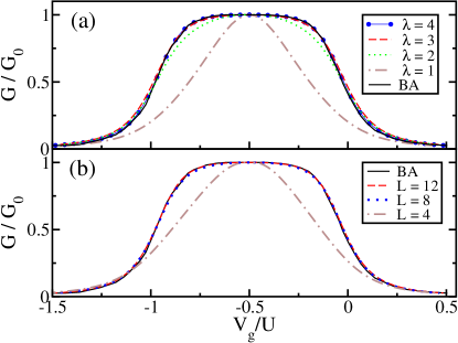
Figure 5: (Color online) Comparison of LDECA and BA. Conductance vs. $V_{\rm g}$ for $U=0.96$ and $t^{\prime}=0.2$. (a) LDECA for $L=12$ and the values of $\lambda$ indicated. (b) LDECA for $L=4$, $8$, and $12$, with $\lambda=4$. The BA result is the solid black line in both (a) and (b).bethe

It is also interesting to note that the improvement of the conductance results for $\lambda>1$ as compared to $\lambda=1$ are associated with a better ‘pinning’ of the Kondo peak to the Fermi energy. This can be partially inferred from the LDOS results shown in Fig. 4(b), where the two solid curves have the Kondo peak pinned at the Fermi energy. This statement can be made more quantitative by considering the results in the inset of Fig. 4(b), showing a comparison between $\lambda=1$ and 2. In that inset, the solid (black) curve is an enlarged view of the LDOS at the vicinity of the Fermi energy for the $V_{g}/U=-0.24$ curve presented in panel (b), which was calculated with $\lambda=2$. The dashed (blue) curve has been calculated with the same parameters, but for $\lambda=1$. The comparison clearly shows that the $\lambda=2$ result has more spectral weight at the Fermi energy than the $\lambda=1$ result. This increase of the spectral weight in the LDOS is at the heart of the improvement achieved for the conductance by using the band discretization.

IV Results: LDECA and a Two-Stage Kondo System

IV.1 Overview: Regimes of the model

We next analyze a system composed of a double-dot side-connected to a lead. The inter-dot and dot-lead connections are given by the matrix elements $t^{\prime\prime}$ and $t^{\prime}$, respectively, as sketched in Fig. 2(b). The transformation to symmetric and antisymmetric states is applied, since we again deal with a one-channel Kondo problem. After performing that transformation, the Hamiltonian is given by:

$$H_{T} = V_{g}\sum_{d,\sigma}n_{d\sigma}+U/2\sum_{d,\sigma}n_{d\sigma}n_{d\bar{\sigma}}$$ (16)

$$+t^{\prime}\sqrt{2}\sum_{\sigma}(c_{d_{2}\sigma}^{\dagger}c_{1\sigma}+c_{1\sigma}^{\dagger}c_{d_{2}\sigma})+H_{\mbox{\small band}}$$

$$H_{\mbox{\small band}} = \sum_{i=1\sigma}^{\infty}t_{i}(c_{i\sigma}^{\dagger}c_{i+1\sigma}+c_{i+1\sigma}^{\dagger}c_{i\sigma})\,,$$

where we use the $t_{i}$ as given in Eq. (12), and $d=d_{1},d_{2}$, labeling dot 1 and dot 2, respectively.

The transport properties of this two-dot system can be expected to be controlled by the interplay between the Kondo effect and the antiferromagnetic inter-dot correlation, and by the interference arising from the two distinct paths available to the electrons: visiting or bypassing the dots.Grempel

As previously discussed in the literature, systems similar to the one depicted in Fig. 2(b), such as, for instance, the so-called T-configuration,Grempel ; zitko06 exhibit two distinct regimes depending on the ratio $t^{\prime\prime}/t^{\prime}$: (i) when $t^{\prime\prime}\gg t^{\prime}$, one is in the molecular regime and (ii) for $t^{\prime\prime}\ll t^{\prime}$, the system crosses over into the TSK regime. It is important to realize that independently of $t^{\prime\prime}$, we expect perfect conductance at $V_{g}=-U/2$. Indeed, at the particle-hole symmetric point the dots always form a singlet, which is of different nature though, depending on the ratio $t^{\prime\prime}/t^{\prime}$, as explained below.

In the molecular regime, on the one hand, both dots act as a single entity, in a way that, as a function of the gate potential, whenever an overall finite magnetic moment is located in the structure, the system exhibits a single-stage Kondo effect. In this regime of $t^{\prime\prime}\gg t^{\prime}$, the system essentially behaves as a single-dot with the two relevant levels separated by a large energy. On the other hand, in the limit of a small $t^{\prime\prime}/t^{\prime}$, such that the effective antiferromagnetic spin-spin interaction between the dots satisfies $J$=$4(t^{\prime\prime})^{2}/U<T_{\rm K}$, the system is in the two-stage Kondo regime, which is characterized by a new energy scale $T_{0}$ related to dot $1$, much lower than the Kondo temperature $T_{\rm K}$ associated to dot $2$. For $T<T_{0}$, very low energy physics is involved,two-stage ; Grempel difficult to be captured by numerical methods such as standard ECA or DMRG. Yet, as shown below, a correct result for the conductance can be obtained from LDECA.

Note that TSK behavior may manifest itself both as a function of temperature at a fixed gate potentialGrempel and as a function of gate potential at a fixed temperature.zitko06 As our method is a zero-temperature one, we will here focus on the gate potential dependence of the conductance and other quantities. We will argue that as one starts from the empty orbital regime, first a single Kondo effect emerges at $V_{g}\gtrsim 0$, which causes a suppression of the conductance. As the gate potential is further tuned towards $V_{g}=-U/2$, the magnetic moment of dot 1 is eventually Kondo-screened as well through the quasi-particles of the composite system of dot 2 and the lead. This gives rise to the aforementioned singlet between dots 1 and 2, which leads to perfect conductance at $V_{g}=-U/2$.

The plan of this section Sec. IV is thus the following. We first demonstrate in Sec. IV.2 that indeed, a singlet is formed between the two dots, independently of $t^{\prime\prime}/t^{\prime}$. These results are obtained with both DMRG and a diagonalization of the bare clusters, before the embedding process. Second, we compute the conductance and charge as a function of gate potential and discuss these results both in the molecular and the TSK regimes in Secs. IV.3 and IV.4, respectively. We further aim at illustrating how the properties of the system change as it crosses over from the molecular regime into the TSK regime. Finally, at particle hole symmetry ($V_{g}=-U/2$), we present LDECA results for the LDOS at the dots and the conductance as a function of $t^{\prime\prime}/t^{\prime}$. As a key result, we demonstrate that using the discretization of the band, LDECA produces perfect conductance down to very low values of $t^{\prime\prime}/t^{\prime}$, a result which was previously out of reach for ECA ($\lambda=1$).

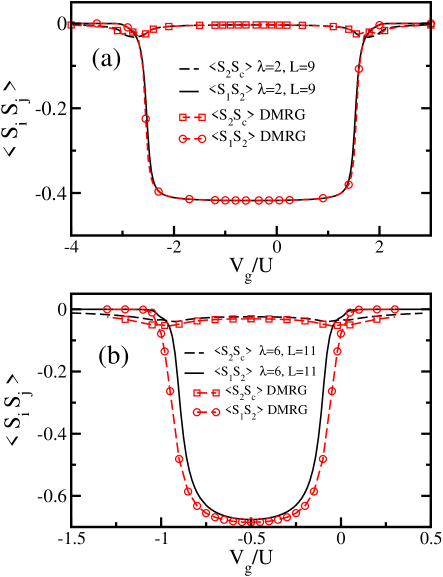
Figure 6: (Color online) Spin-spin correlations calculated by Lanczos and DMRG as a function of $V_{\rm g}$ for $U=1.0$ and $t^{\prime}=0.3$. (a) $t^{\prime\prime}=2.0$ (molecular regime) and (b) $t^{\prime\prime}=0.05$ (TSK regime). Lanczos with $L=11$ and $\lambda=6$, $\langle{\bf S}_{1}\cdot{\bf S}_{2}\rangle$ (solid) and $\langle{\bf S}_{2}\cdot{\bf S}_{c}\rangle$ (dashed) black lines; DMRG with $196$ sites at half filling of the full system and $\lambda=1$, $\langle{\bf S}_{1}\cdot{\bf S}_{2}\rangle$ (circles) and $\langle{\bf S}_{2}\cdot{\bf S}_{c}\rangle$ (squares).

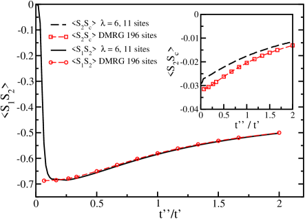
Figure 7: (Color online) Spin-spin correlations as a function of $t^{\prime\prime}/t^{\prime}$ for $U=1.0$, $t^{\prime}=0.3$ and $V_{\rm g}=-U/2$. See legend and Fig. 6 for the description of the lines.

IV.2 Spin-spin correlations

For the present model, we now establish the presence of a strong antiferromagnetic correlation between the dots by analyzing the spin-spin correlations as a function of $V_{\rm g}$, presented in Fig. 6 for both $t^{\prime\prime}=2.0$ (upper panel) and $t^{\prime\prime}=0.05$ (lower panel), with $t^{\prime}=0.3$ in both cases. Results are for large clusters with $196$ sites and $\lambda=1$, obtained with DMRG, and also for $L=9$ and $\lambda=2$ (upper panel), and for $L=11$ and $\lambda=6$ (lower panel), using a Lanczos diagonalization procedure. Both DMRG and Lanczos calculations were done without embedding.

In the case of the molecular regime [$t^{\prime\prime}=2$, Fig. 6(a)], the inter-dot correlation $\langle{\bf S}_{1}\cdot{\bf S}_{2}\rangle$ is large for $-2.5\lesssim V_{g}/U\lesssim 1.5$. Therefore, we expect a perfect conductance in that window, and a Kondo anti-resonance to appear at $V_{g}/U\gtrsim 1.5$ (see Fig. 9(a), below). For the smaller $t^{\prime\prime}=0.05$ [Fig. 6(b)], the antiferromagnetic correlation between the dots is dominant in the window $-U<V_{\rm g}<0$, indicating the formation of a singlet. While the inter-dot spin correlation $\langle{\bf S}_{1}\cdot{\bf S}_{2}\rangle$ is large at the electron-hole symmetric point $V_{\rm g}=-U/2$, the antiferromagnetic correlation $\langle{\bf S}_{2}\cdot{\bf S}_{c}\rangle$, although small, is not zero. Note that site c is adjacent to dot 2, see Fig. 2(b). For instance, $\langle{\bf S}_{2}\cdot{\bf S}_{c}\rangle$ takes a maximum at $V_{g}\approx 0$ in the case of $t^{\prime\prime}=0.05$, indicative of the single-stage Kondo effect that is observed in that gate potential region [see Fig. 11(a)].

We now study both correlations as a function of $t^{\prime\prime}/t^{\prime}$ at $V_{g}=-U/2$, which is displayed in Fig. 7. An important observation is that $\langle{\bf S}_{2}\cdot{\bf S}_{c}\rangle$ increases in magnitude as $t^{\prime\prime}$ is reduced, as is shown in the inset of Fig. 7. This fact indicates the subtle existence of a Kondo-like ground state, which is strengthened when $t^{\prime\prime}$ is reduced. In addition, the antiferromagnetic inter-dot correlation, presented in the main panel of Fig. 7, also increases when $t^{\prime\prime}$ is reduced, taking values as large as $\langle{\bf S}_{1}\cdot{\bf S}_{2}\rangle\approx-0.7$, for $t^{\prime\prime}/t^{\prime}\gtrsim 1/10$. This is surprising, since the interplay of these two correlations has a behavior opposite to other known systems, such as heavy fermions near a quantum phase transition Coqblin or embedded two-dot nanostructures.Busser1 It reflects the existence of an inter-dot singlet for all values of $t^{\prime\prime}$$>$0. However, the nature of the singlet for small $t^{\prime\prime}/t^{\prime}$ is different from that for the large $t^{\prime\prime}/t^{\prime}$ regime. While in the latter case the singlet, which is caused by the direct interaction between the dots, destroys the Kondo regime, in the former case it is enhanced by the Kondo spin correlation with the intervention of the conduction electrons, as shown by the fact that the inter-dot and the Kondo spin correlations increase when $t^{\prime\prime}$ is reduced. These results illustrate the characteristics of a TSK state. The comparison of data from large clusters ($196$ sites, $\lambda=1$) and short ones ($L=11$, $\lambda=6$) yields a convincing agreement for the spin correlations, especially for $\langle{\bf S}_{1}\cdot{\bf S}_{2}\rangle$, governing the inter-dot singlet. This agreement indicates that the spin-spin correlations are, so to speak, localized objects. The embedding process is not as important to calculate static properties as it is for the conductance, which we shall see later. Still, the vanishing of $\langle{\bf S}_{1}\cdot{\bf S}_{2}\rangle$ at very small $t^{\prime\prime}/t^{\prime}$ on the smaller cluster reflects that, in this particular limit, the embedding is crucial to overcome this finite-size effect. An important point that we want to emphasize here is that the molecular and TSK results suggest perfect conductance at $V_{\rm g}=-U/2$ for any nonzero $t^{\prime\prime}$.

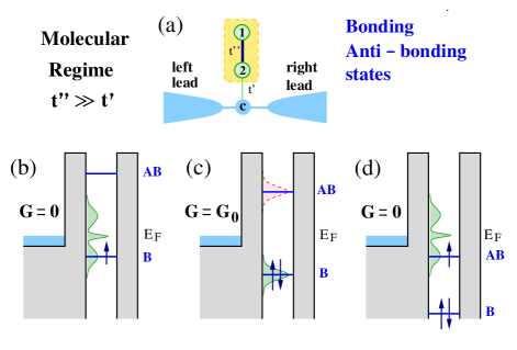
Figure 8: (Color online) Schematic representation of the molecular regime. (a) When $t^{\prime\prime}\gg t^{\prime}$, the two dots form a single entity, represented by the shaded box. (b) - (d) Different regimes at different values of gate potential: (b) Kondo effect for the bonding orbital (zero conductance, because of the back-scattering density of states at the Fermi energy $E_{\rm F}$), (c) Perfect conductance at $V_{g}=-U/2$ (no back-scattering density of states at $E_{\rm F}$), (d) Kondo effect for the anti-bonding orbital (zero conductance).

IV.3 Molecular regime

We proceed with an analysis of the conductance for the so-called ‘molecular’ regime. In Fig. 8(a), we schematically illustrate what happens for $t^{\prime\prime}/t^{\prime}\gg 1.0$, i.e., when the independent dots are ‘locked’ into ‘molecular’ bonding and anti-bonding orbitals, separated by a large energy, proportional to $t^{\prime\prime}$. The two dots now behave as a single structure, represented by the dashed square box, side-connected to the leads. The effect of these molecular orbitals over the conductance through the leads, as the gate potential $V_{g}$ varies, is pictured in panels (b) to (d), where now the bonding and anti-bonding orbitals are depicted inside a quantum well. In panel (b), the bonding orbital is in the Kondo regime. As the double-dot structure is side-connected to the leads, the conduction electrons are back-scattered, resulting in zero conductance. note-inter Panel (c) shows that, at the particle-hole symmetric point $V_{g}=-U/2$, the bonding orbital is doubly occupied, lying below the Fermi energy ${\rm E_{\rm F}}$, and the anti-bonding orbital, lying above ${\rm E_{\rm F}}$, is empty. Therefore, in this case, the double-dot structure creates no back-scattering density of states at ${\rm E_{\rm F}}$ [as schematically indicated in the panel (c)], resulting in perfect conductance. Finally, panel (d) displays the corresponding Kondo effect for the anti-bonding orbital, also resulting in zero conductance.

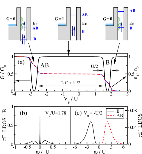
Figure 9: (Color online) (a) Conductance and charge as a function of $V_{\rm g}$ for the molecular regime ($U=1.0$, $t^{\prime}=0.3$, and $t^{\prime\prime}=2.0$) for the two side-connected quantum dots. Notice that each feature of the conductance is associated to the respective diagram introduced in Fig. 8. Panel (b) displays the LDOS for the bonding state (B) for $V_{\rm g}/U=1.78$ (the anti-bonding state (AB) has an identical peak for $V_{\rm g}/U=-2.78$). Panel (c) displays the LDOS for the bonding (solid (black) line) and anti-bonding (dashed (red) line) states at the particle-hole symmetric point $V_{g}=-U/2$. $\lambda=2$ for all calculations.

Figure 9 shows the conductance and the charge vs. gate voltage in the molecular regime as obtained with LDECA for $t^{\prime\prime}=2.0$, $t^{\prime}=0.3$, and $U=1$ on a cluster with $L=11$ sites and $\lambda=2$. In this plot, one observes the two Fano-Kondo anti-resonances, with an approximate width of $U/2$, originating from two ‘molecular’ levels separated by $\approx 2\times t^{\prime\prime}+U/2$. It is important to emphasize that in the molecular regime the two dots behave as a unique entity, providing an extra lateral path for the electrons to traverse when visiting the Kondo peak derived from the molecular orbital. This gives rise to the Fano antiresonance in the conductance appearing in Fig. 9(a). As expected, both dots are charged almost simultaneously, as one can see in Fig. 9(a), with a dashed line for dot 1 and a solid thin line for dot 2. In the top of Fig. 9, the corresponding potential wells described in Fig. 8 are displayed.

To illustrate the idea of a ‘molecular orbital Kondo effect’, in the lower left panel, we display the LDOS associated with the molecular bonding orbital formed with the two dots. This LDOS is calculated at the positive gate potential at which the conductance is zero, which turns out to be at $V_{g}\approx t^{\prime\prime}-U/4$, as expected. We find the ‘molecular’ Kondo peak at the Fermi energy, as well as the broadened $\epsilon$ and $\epsilon+\tilde{U}$ levels, where the renormalized intra-orbital Coulomb repulsion $\tilde{U}=U/2$ can be obtained by rewriting the dot Coulomb repulsion in the basis of the bonding and anti-bonding orbitals. A similar result (not shown) is found for the LDOS of the antibonding orbital at the $V_{g}$ value for which the second Kondo-Fano resonance occurs. The LDOS for each quantum dot (not shown) also exhibits a Kondo peak. Indeed, since the two dots equally participate in the molecular Kondo effect, their LDOS are quite similar to each other, and qualitatively similar to what is shown in Fig. 9(b). Finally, in Fig. 9(c), we show the LDOS for both the bonding and anti-bonding orbitals for $V_{g}=-U/2$, where clearly the Kondo peak is absent and the two orbital levels are separated by about $2t^{\prime\prime}$.

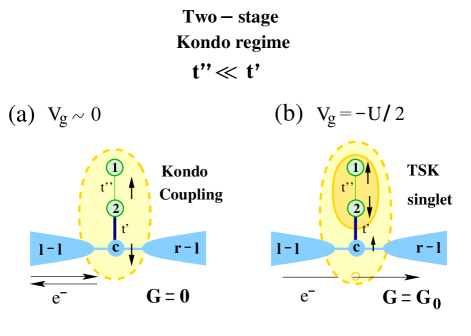
Figure 10: (Color online) Schematic representation of the TSK regime, obtained when $t^{\prime\prime}\ll t^{\prime}$. (a) Sketch of the first Kondo stage, when the two dots are occupied by a single electron, which forms a Kondo singlet with the conduction electrons, represented by the vertical antiparallel arrows (one in the dots, the other in the band). The Kondo coupling, which mediates the formation of the many-body singlet, is represented by the (yellow) lightly shaded oval. The density of states created by the Kondo effect in dot 2 at the Fermi energy induces backward scattering of the conduction electrons going through the leads (horizontal antiparallel arrows). This results in zero conductance. (b) At $V_{g}=-U/2$, when the dots have total charge $n=2$, the spins in the dots are locked into a singlet (darker shaded oval). This singlet is mediated through two Kondo effects, represented by the underlying lighter (yellow) oval. The combination of these two Kondo effects, in contrast to the case in panel (a), removes density of states from dot 2 exactly at the Fermi energy, suppressing the back-scattering and resulting in perfect conductance. This is represented by the rightward arrow ‘piercing’ the Kondo coupling oval.

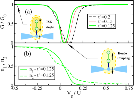
Figure 11: (Color online) (a) Conductance and (b) charge in the dots as a function of $V_{\rm g}$ for values of $t^{\prime\prime}<t^{\prime}$ ($U=1.0$, $t^{\prime}=0.3$, and values of $t^{\prime\prime}$ as indicated). See text for discussion. All calculations are for $\lambda=2.0$, except for $t^{\prime\prime}=0.125$, where $\lambda=\sqrt{6}$. Notice that the conductance and charge features at $V_{g}\approx 0$ and $V_{g}=-U/2$ were associated to the schematic diagrams introduced in Fig. 10.

IV.4 Two-stage Kondo regime

Figure 10 schematically depicts a much more subtle regime than that of Fig. 8, the TSK regime. One enters into this regime when $t^{\prime\prime}\ll t^{\prime}$, where now the connection of dot 2 with the leads is much stronger than the inter-dot connection. Here, the concept of bonding and anti-bonding orbitals does not apply, since each dot feels the interaction with the conduction electrons differently, the crucial point being that dot 1 interacts with the Fermi sea through dot 2.

In this and the next section, we will present evidence that our LDECA results are perfectly consistent with the notion of TSK behavior. As a guidance to interpreting the numerical results, this behavior can be schematically described as follows. In Fig. 10(a), where the gate potential $V_{g}$ is such that the charge occupancy of the two dots is 1, i.e., $n_{1}+n_{2}=1$, a Kondo effect develops, represented by the oval shape with dashed borders, resulting in back-scattering and a vanishing conductance, as indicated by the horizontal arrows. The Kondo effect involves a magnetic moment located in the dots, which is screened by the conduction electrons, indicated by the arrow on the dot and an antiparallel one in the band. In Fig. 10(b), depicting the situation for $V_{g}=-U/2$, the two dots are each singly occupied and a strong singlet forms between them, represented by the darker oval shape with a solid border. Although in this regime the LDOS of dot 2 is exactly zero at the Fermi energy, therefore suppressing the back-scattering and restoring perfect conductance (this is represented by the arrow ‘piercing’ the lighter shaded oval), it does not eliminate the Kondo spin-spin correlation between the spin of dot 2 and the conduction spins. On the one hand, the conduction electrons do not see the two dot system as a unique entity: Indeed, they recognize dot 2 as a separate object to which their spins correlate. On the other hand, the spin of dot 1 sees the rest of the system as a whole, and Kondo correlates with the spin of dot 2, thus creating the two-dot singlet state. In reality, the singlet is a many-body effect involving the conduction electrons and it is composed of two consecutive Kondo effects (represented here by the underlying lightly shaded oval).

In Fig. 11, we show the LDECA conductance [panel (a)] and the charge in each dot [panel (b)] as a function of $V_{g}$ for much lower values of $t^{\prime\prime}$ than in the previous molecular regime, namely $t^{\prime\prime}=0.2$, $0.15$, and $0.125$. Let us first discuss the charge, as an example of a quantity that exhibits a qualitatively different behavior for high and low values of $t^{\prime\prime}/t^{\prime}$, with the two dots behaving more independently as $t^{\prime\prime}\to 0$.

In the small $t^{\prime\prime}/t^{\prime}$ regime, dot 2 is charged first upon approaching $V_{g}=0$, and only when it has a substantial amount of charge dot 1 starts to be charged as well [see Fig. 11(b)]. In addition, around $V_{g}\approx 0$ where the minimum in the conductance occurs due to the single-stage Kondo effect, the curve for the charge of dot 2 features a much more well defined plateau than that for dot 1. This indicates that, in contrast to the molecular regime [see charge behavior in Fig. 9(a)], the two dots now start to have a qualitatively different participation in the Kondo effect, suggesting that at this much lower value of $t^{\prime\prime}/t^{\prime}$ and at $V_{g}\approx 0$, one starts to see the emergence of the first stage of the TSK regime. (Notice that DMRG results for the charge and the total spin as a function of $V_{g}$ for large clusters (not shown) agree with the LDECA picture just described). In addition, the width of the Kondo anti-resonance seen in Fig. 11(a) is now substantially smaller than $U/2$, which is the typical value found in the molecular regime, see Fig. 9(a), although much larger than the intrinsic width of the dots’ resonance states. Finally, as one approaches $V_{g}=-U/2$, and each dot now has one electron, the second stage of the TSK is reached. In this regime, through the mediation of the conduction electrons, the interdot-singlet is formed and, although it shows a two-Kondo peak structure, the LDOS of dot 2 is zero at the Fermi energy [see Fig. 13(b)]. As a consequence, the system exhibits perfect conductance [see Fig. 11(a)].

IV.5 Conductance and LDOS at $V_{g}=-U/2$

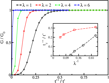
Figure 12: (Color online) Conductance vs. $t^{\prime\prime}/t^{\prime}$ for $U=1.0$, $t^{\prime}=0.3$, $V_{g}=-U/2$. Results are for $L=11$ and $\lambda=1$ (black circles), $\lambda=2$ (red squares), $\lambda=4$ (green diamonds) and $\lambda=6$ (blue triangles). In the inset, we show $t^{\prime\prime}_{c}(\lambda)/t^{\prime}$ for $L=11$ (black circles) and $L=5$ (red squares).

Next, we discuss the conductance at the particle-hole symmetric point as a function of $t^{\prime\prime}$ to show that LDECA correctly captures the low-energy physics down to small values of $t^{\prime\prime}$.

Figure 12 displays the conductance vs. $t^{\prime\prime}$ for various values of $\lambda$ and $L=11$. We recall that, as exemplified in Figs. 9 and 11, the conductance at $V_{g}=-U/2$ for any $t^{\prime\prime}>0$ should be $G=G_{0}$. We study the electron-hole symmetry situation, as it is the most difficult point to be correctly described, having the lowest Kondo temperature for the set of parameters taken. The suppression of the conductance for small values of $t^{\prime\prime}/t^{\prime}$ shown in Fig. 12 is caused by finite-size effects which obscure the second stage Kondo effect. In this specific case, we find the tendency of a strong suppression of spin fluctuations in dot 1 as the system approaches half-filling, ($V_{g}=-U/2$). This behavior at $\lambda=1$ is similar to other models discussed in detail in Ref. hm08, . Figure 12 suggests that the finite-size dependence of the conductance for $\lambda=1$ (circles) is quite severe, as it starts to manifest itself at $t^{\prime\prime}/t^{\prime}\approx 0.5$. However, it is also evident that by increasing $\lambda$ the situation improves markedly, which is the main message to be taken from this figure.

From the curves for each different $\lambda$ we can extract a characteristic inter-dot coupling $t_{c}^{\prime\prime}(\lambda)$, satisfying $G(t_{c}^{\prime\prime})/G_{0}=1/2$, below which the conductance rapidly approaches zero. The dependence of $t^{\prime\prime}_{c}$ on $\lambda^{-1}$ for two different values of $L$ is shown in the inset. $t_{c}^{\prime\prime}(\lambda)$ tends to zero for values of $\lambda$ that decrease with increasing cluster size. Therefore, at $V_{\rm g}$=$-U/2$, $G/G_{0}\to 1$ when $t^{\prime\prime}\to 0$.

To further demonstrate the difference between the molecular and the TSK regimes at $V_{g}=-U/2$, Fig. 13 shows a comparison between the LDOS for two widely different values of $t^{\prime\prime}/t^{\prime}$. In Fig. 13(a), we show the LDOS at dot 2 for $t^{\prime\prime}=2.0$, $t^{\prime}=0.3$, $U=1.0$, and $\lambda=2$. These are the same parameters as the ones used in Fig. 9(c), where the bonding and anti-bonding orbitals where shown. Figure 13(a) unveils why the conductance in the molecular regime is $G=G_{0}$ at $V_{g}=-U/2$ [see Fig. 9(a)], as dot 2 has a vanishing density of states in a wide energy region around the Fermi level. Once there is no back-scattering density of states at the Fermi energy, the conductance is perfect.

On the other hand, in Fig. 13(b), LDOS results for dot 2 are depicted for $t^{\prime\prime}=5^{-2}$, and $\lambda=\sqrt{6}$, and the same values of $t^{\prime}$ and $U$ as in Fig. 13(a). Again, the density of states at the Fermi energy vanishes. However, in this case, close to the Fermi energy, we find two sharp features, suggestive of a Kondo peak split in two. To substantiate this picture, the dashed (red) curve in Fig. 13(b) shows the Kondo peak that is present when $t^{\prime\prime}=0$, i.e., when dot 1 is effectively removed. It is the presence of dot 1, interacting with the rest of the system through dot 2, that gives rise to the TSK regime, reflected in the LDOS of dot 2 as an antiresonance in the middle of its Kondo peak.

In summary, the fact that the Kondo regime of dot 1 is mediated by the Kondo state of dot 2 explains the surprising result of a perfect conductance at $V_{g}=-U/2$ in the TSK regime. This mechanism reduces the LDOS at the Fermi level of dot 2 to zero as shown in Fig. 13(b), eliminating an alternative path for the circulating electrons and hence any destructive interferences. In this regime, the electrons at the dots form a spin singlet, even at small $t^{\prime\prime}/t^{\prime}$. This subtle effect and its consequences on the conductance are well captured by LDECA. It is then clearly shown in Figs. 12 and 13 that the logarithmic discretization of the band, combined with the embedding process, provides reliable results in a wide parameter range.

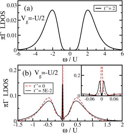
Figure 13: (Color online) (a) LDOS at dot 2 for $L=11$, $t^{\prime\prime}=2$, $t^{\prime}=0.3$, $U=1$, $V_{g}=-U/2$, and $\lambda=2$ (same parameters as the ones in Fig. 9(c), but here we show the LDOS of dot 2 only). Notice the large region of vanishing LDOS around the Fermi energy ($\omega=0$). (b) Same as in (a), but now for $t^{\prime\prime}=5\times 10^{-2}$ and $\lambda=\sqrt{6}$ (solid (black) line). Notice that, as in (a), the LDOS vanishes at the Fermi energy, but now only in a very narrow interval. A comparison of the width of the double-peak structure at low $\omega$ with the LDOS results for $t^{\prime\prime}=0$ (dashed (red) line), i.e., for a single side-connected dot, suggests that the double-peak structure is a split Kondo peak. An enlarged view of the double-peak structure is seen in the inset.

V Summary

In this paper, we developed a formalism to study local and highly correlated electrons that combines the numerical simplicity of the ECA method with Wilson’s idea of a logarithmic discretization of the non-interacting band. A diagrammatic expansion that provides a solid theoretical basis for the method was also discussed. Applied to a one-impurity problem, LDECA yields an excellent agreement with BA results. In addition, following the same procedure used in NRG to broaden the LDOS, a perfect agreement was found with the accepted results for the LDOS of the Anderson impurity model. In the case of a double-dot side-connected to a lead, and at small $t^{\prime\prime}$, the contrast between the $\lambda$=$1$ (ECA) and $\lambda>1$ (LDECA) results exemplifies the power of the logarithmic discretization: the low-energy physics associated to the TSK regime is correctly unveiled, as LDECA provides an accurate description of the physics close to the Fermi energy.

The main advantage of LDECA is its great flexibility, which allows the incorporation of other degrees of freedom, such as localized phonons or photons.Guille The restrictions imposed by the Lanczos method can be overcome by using DMRG,white allowing one to use larger systems and to study more involved problems. Related efforts are in progress.

We conclude that the LDECA method can be applied to complex problems, including molecules adsorbed at a metallic surface quique and sophisticated topologies of quantum dots, displaying exotic Kondo regimes, such as, for example, non-Fermi liquid behavior, two-channel Kondo effect and the physics associated to SU(N) systems.

Acknowledgments - We thank K.A. Al-Hassanieh, L.G.G.V. Dias daSilva, E. Louis, V. Meden, N. Sandler, A. Schiller, and J. A. Verges for helpful discussions. E.V.A. and M.A.D. acknowledge the support of FAPERJ and CNPq (Brazil). G.Ch. acknowledges financial support by the Spanish MCYT (grants FIS200402356, MAT2005-07369-C03-01 and NAN2004-09183-C10-08 and a Ramón y Cajal fellowship), the Universidad de Alicante and the Generalitat Valenciana (grant GRUPOS03/092). E.D. and F.H.-M. were supported by the NSF grant DMR-0706020 and by the Division of Materials Science and Engineering, U.S. DOE under contract with UT-Battelle, LLC. G.B.M. acknowledges support from NSF (DMR-0710529) and from Research Corporation (Contract No. CC6542).

Appendix A Diagrammatic Expansion

In this appendix we develop the diagrammatic expansion of the one particle Green function at the impurity site given by

$$G_{00,\sigma}(t-t^{\prime})=\frac{\left\langle\mathcal{T}\{c_{0\sigma}(t)c^{\dagger}_{0\sigma}(t^{\prime})S(\infty)\}\right\rangle_{0}}{\left\langle S(\infty)\right\rangle_{0}}\,,$$ (17)

where, as usual, $S(\infty)$ is the evolution operator and $\mathcal{T}$ is the time order operator. The mean values are calculated in the ground state of the unperturbed Hamiltonian $H_{0}$, given by Eq. (4), restricting our discussion to zero temperature.

The evolution operator $S(\infty)$ is expanded in increasing orders of the perturbing term $H_{\mbox{\small p}}$, which, when inserted in Eq. (17), gives rise to a perturbation series for the Green function. It can be written as

$$S(\infty)=\sum^{\infty}_{n=1}\frac{-i^{n}}{n!\big{<}S(\infty)\big{>}}\int^{t}_{t_{0}}\ldots\int^{t}_{t_{0}}\left\langle\mathcal{T}\left\{c_{0\sigma}(t)H_{\mbox{\small p}}(t_{1})\ldots H_{\mbox{\small p}}(t_{n})\right\}c^{\dagger}_{0\sigma}(t^{\prime})\right\rangle_{0}dt\ldots dt_{n}\,.$$ (18)

Substituting this expression into Eq. (17), the local Green function is given by

$$G_{00,\sigma}(t-t^{\prime}) =g_{0,\sigma}(t-t^{\prime})+V^{2}\sum_{\sigma_{1}\sigma_{2}}\int g_{0,N,N+1,\sigma,\sigma_{1},\sigma_{2}}(t,t_{1},t_{2},t^{\prime})dt_{1}dt_{2}$$ (19)

$$+V^{4}\sum_{\sigma_{1}\sigma_{2}\sigma_{3}\sigma_{4}}g_{0,N,N+1,\sigma,\sigma_{1},\sigma_{2},\sigma_{3},\sigma_{4}}(t,t_{1},t_{2},t_{3},t_{4},t^{\prime})dt_{1}dt_{2}dt_{3}dt_{4}+$$

$$+\cdots\,.$$

It is important to emphasize, as shown in Eq. (19), that the conservation of charge of the unperturbed subsystem restricts the expansion to even orders in $V$. The undressed Green function appearing in the equation is defined as

$$\begin{array}[]{l}g_{0,N,N+1,\sigma,\sigma_{1},\sigma_{2}}(t,t_{1},t_{2},t^{\prime})=\\ \\ \left\langle\!\mathcal{T}\!\!\left\{\!c_{0\sigma}\!(t)c^{\dagger}_{N\sigma_{1}}\!(t_{1}\!)c_{N+1\sigma_{1}}\!(t_{1}\!)c^{\dagger}_{N+1\sigma_{2}}\!(t_{2}\!)c_{N\sigma_{2}}\!(t_{2}\!)c^{\dagger}_{0\sigma}\!(t^{\prime})\!\right\}\!\right\rangle_{0}\end{array}$$ (20)

with an obvious generalization for the undressed Green function of other orders. Calculating terms of all orders in $V$ in the expansion, Eq. (19), the local Green function can be written as

$$G_{00,\sigma}(t-t^{\prime})\!=\!G^{(0)}_{00,\sigma}(t-t^{\prime})+G^{(2)}_{00,\sigma}(t-t^{\prime})+G^{(4)}_{00,\sigma}(t-t^{\prime})+\cdots.$$ (21)

As the operators belonging to the two different unperturbed parts of the system are, in this ground state, decoupled from each other since there is no connection between the cluster and the rest of the leads, Eq. (20) results in

$$g_{0,N,N+1,\sigma,\sigma_{1},\sigma_{2}}(t,t_{1},t_{2},t^{\prime})$$

$$=g_{0,N,\sigma,\sigma_{1}}(t,t_{1},t_{2},t^{\prime})g_{N+1,\sigma_{1}}(t_{1},t_{2})\delta_{\sigma_{1}\sigma_{2}}$$ (22)

where the spin conservation imposes the condition $\sigma_{1}=\sigma_{2}$ and

$$g_{0,N,\sigma,\sigma_{1}}\!(t,t_{1},t_{2},t^{\prime})\!\!\! = \!\!\!\left\langle\!\mathcal{T}\{c_{0,\sigma}(t)c^{\dagger}_{N,\sigma_{1}}\!(t_{1}\!)c_{N,\sigma_{1}}\!(t_{2})c^{\dagger}_{0,\sigma}(t^{\prime})\!\}\!\!\right\rangle_{\!\!0}$$

$$g_{N+1,\sigma_{1}}\!(t_{1},t_{2})\!\!\! = \!\!\!\left\langle\mathcal{T}\{c_{N+1,\sigma_{1}}\!(t_{1}\!)c^{\dagger}_{N+1,\sigma_{1}}\!(t_{2})\}\right\rangle_{0}\,.$$ (23b)

According to Eq. (22), the expansion Eq. (19) is formally a locator-propagator expansion metzner where the locators correspond to the unperturbed sub-systems Green functions and the propagator turns out to be the one connecting them.

The Green function $g_{0,N,\sigma,\sigma_{1}}$ can be diagrammatically represented by

$$g_{0,N,\sigma,\sigma_{1}}(t,t_{1},t_{2},t^{\prime}) = \sigma_{1} t_{1} t_{2} \sigma_{1} t \sigma t^{\prime}$$

$$\mathcal{T}\left\{c_{o\sigma}(t)c^{\dagger}_{N\sigma_{1}}(t_{1})c_{N\sigma_{1}}(t_{2})c^{\dagger}_{o\sigma}(t^{\prime})\right\}$$

and

$$g_{N+1,\sigma}(t_{1},t_{2})=\hskip 36.98866pt\begin{picture}(0.0,0.0)(40.0,0.0)\put(7.0,2.0){\circle*{6.0}} \put(7.0,2.0){\lx@xy@svg{\hbox{\raise 0.0pt\hbox{\kern-5.69052pt\hbox{\ignorespaces\ignorespaces\ignorespaces\ignorespaces{}\ignorespaces\ignorespaces\ignorespaces{\hbox{\lx@xy@drawsquiggles@}}\ignorespaces{}\ignorespaces\ignorespaces\ignorespaces{\hbox{\lx@xy@drawsquiggles@}}\ignorespaces{\hbox{\lx@xy@drawsquiggles@}}\ignorespaces}}}}} \put(36.0,2.0){\circle*{6.0}} \put(3.0,10.0){$t_{1}$} \put(18.0,10.0){$\sigma$} \put(34.0,10.0){$t_{2}$} \end{picture}\mathcal{T}\left\{c_{N+1\sigma_{1}}(t_{1})c_{N+1\sigma_{1}}(t_{2})\right\}$$

The zeroth-order contribution to the Green function, i.e., the solution of the problem for $V=0$, is represented in terms of diagrams as

$$G_{00,\sigma}^{(0)}(t-t^{\prime})=\left\langle\mathcal{T}\left\{c_{0\sigma}(t)c^{\dagger}_{0\sigma}(t^{\prime})\right\}\right\rangle_{0}=\put(8.0,3.0){\line(1,0){10.0}}\put(5.0,3.0){\circle{6.0}}\put(18.0,1.0){\framebox(26.0,5.0)[]{}}\put(44.0,3.0){\line(1,0){10.0}}\put(57.0,3.0){\circle{6.0}}\put(3.0,-9.0){$t$}\put(26.0,-9.0){$\sigma$}\put(52.0,-9.0){$t^{\prime}$}\qquad\qquad\qquad$$ (24)

The Green function is exactly obtained by calculating the ground state of the cluster using the Lanczos method. Although it includes the many-body interaction and its effects within the cluster, it is the undressed Green function with respect to the expansion given by Eq. (21).

To second order in perturbation theory, the contribution to $G_{00,\sigma}(t-t^{\prime})$ is

$$G^{(2)}_{00,\sigma}(t-t^{\prime})=\frac{V^{2}}{\left<S(\infty)\right>_{0}}$$

$$\sum_{\sigma_{1}}\!\!\int\!\!g_{0,N,\sigma_{,}\sigma_{1}}(t,t_{1},t_{2},t^{\prime})g_{N+1,\sigma_{1}}(t_{1},t_{2})dt_{1}dt_{2}$$ (25)

and can be diagrammatically represented as

$$G^{(2)}_{00,\sigma}(t-t^{\prime})=\hskip 79.6678pt\begin{picture}(0.0,30.0)(80.0,0.0)\put(8.0,3.0){\line(1,0){10.0}} \put(5.0,3.0){\circle{6.0}} \put(14.0,13.0){$\sigma_{1}$} \put(2.0,-10.0){$t$} \put(13.0,25.0){$t_{1}$} \put(30.0,32.0){$\sigma_{1}$} \put(26.0,25.0){\circle*{6.0}} \put(26.0,6.0){\line(0,1){16.0}} \put(26.0,25.0){\lx@xy@svg{\hbox{\raise 0.0pt\hbox{\kern-5.69052pt\hbox{\ignorespaces\ignorespaces\ignorespaces\ignorespaces{}\ignorespaces\ignorespaces\ignorespaces{\hbox{\lx@xy@drawsquiggles@}}\ignorespaces{}\ignorespaces\ignorespaces\ignorespaces{\hbox{\lx@xy@drawsquiggles@}}\ignorespaces{\hbox{\lx@xy@drawsquiggles@}}\ignorespaces}}}}} \put(50.0,25.0){$t_{2}$} \put(30.0,-9.0){$\sigma$} \put(46.0,25.0){\circle*{6.0}} \put(46.0,6.0){\line(0,1){16.0}} \put(49.0,13.0){$\sigma_{1}$} \put(18.0,1.0){\framebox(37.0,5.0)[]{}} \put(55.0,3.0){\line(1,0){10.0}} \put(68.0,3.0){\circle{6.0}} \put(72.0,-10.0){$t^{\prime}$} \end{picture}\,,$$ (26)

where an integration over each internal time $t_{1}$ and $t_{2}$ is implied and the sum over $\sigma_{1}$ needs to be taken.

Regarding the calculation of the many-particle Green functions at the lead sites outside the cluster, Wick’s theorem can be used since this part of the system is represented by a one-body Hamiltonian. In this case, it is clear that for the fourth order we obtain the diagram

$$G^{(4)}_{00,\sigma}(t-t^{\prime})=\hskip 119.50148pt\begin{picture}(0.0,25.0)(120.0,0.0)\put(8.0,3.0){\line(1,0){10.0}} \put(5.0,3.0){\circle{6.0}} \put(14.0,13.0){$\sigma_{1}$} \put(2.0,-10.0){$t$} \put(13.0,25.0){$t_{1}$} \put(30.0,32.0){$\sigma_{1}$} \put(26.0,25.0){\circle*{6.0}} \put(26.0,6.0){\line(0,1){16.0}} \put(26.0,25.0){\lx@xy@svg{\hbox{\raise 0.0pt\hbox{\kern-5.69052pt\hbox{\ignorespaces\ignorespaces\ignorespaces\ignorespaces{}\ignorespaces\ignorespaces\ignorespaces{\hbox{\lx@xy@drawsquiggles@}}\ignorespaces{}\ignorespaces\ignorespaces\ignorespaces{\hbox{\lx@xy@drawsquiggles@}}\ignorespaces{\hbox{\lx@xy@drawsquiggles@}}\ignorespaces}}}}} \put(50.0,25.0){$t_{2}$} \put(60.0,-9.0){$\sigma$} \put(46.0,25.0){\circle*{6.0}} \put(46.0,6.0){\line(0,1){16.0}} \put(49.0,13.0){$\sigma_{1}$} \put(18.0,1.0){\framebox(90.0,5.0)[]{}} \put(108.0,3.0){\line(1,0){10.0}} \put(121.0,3.0){\circle{6.0}} \put(120.0,-10.0){$t^{\prime}$} \put(65.0,13.0){$\sigma_{2}$} \put(65.0,25.0){$t_{3}$} \put(78.0,25.0){\circle*{6.0}} \put(78.0,6.0){\line(0,1){16.0}} \put(78.0,25.0){\lx@xy@svg{\hbox{\raise 0.0pt\hbox{\kern-5.69052pt\hbox{\ignorespaces\ignorespaces\ignorespaces\ignorespaces{}\ignorespaces\ignorespaces\ignorespaces{\hbox{\lx@xy@drawsquiggles@}}\ignorespaces{}\ignorespaces\ignorespaces\ignorespaces{\hbox{\lx@xy@drawsquiggles@}}\ignorespaces{\hbox{\lx@xy@drawsquiggles@}}\ignorespaces}}}}} \put(80.0,32.0){$\sigma_{2}$} \put(104.0,25.0){$t_{4}$} \put(98.0,25.0){\circle*{6.0}} \put(98.0,6.0){\line(0,1){16.0}} \put(101.0,13.0){$\sigma_{2}$} \end{picture}\,,$$ (27)

such that the dressed locator $G_{00,\sigma}(t-t^{\prime})$ can be cast into

$$G_{00,\sigma}(t-t^{\prime})=\hskip 398.33858pt\begin{picture}(0.0,0.0)(400.0,0.0)\put(8.0,3.0){\line(1,0){10.0}} \put(5.0,3.0){\circle{6.0}} \put(18.0,1.0){\rule{28.45274pt}{5.69054pt}} \put(45.0,3.0){\line(1,0){10.0}} \put(58.0,3.0){\circle{6.0}} \put(3.0,-10.0){$t$} \put(29.0,-10.0){$\sigma$} \put(56.0,-10.0){$t^{\prime}$} \put(65.0,0.0){$=$} \end{picture}\begin{picture}(0.0,0.0)(325.0,0.0)\put(8.0,3.0){\line(1,0){8.2}} \put(5.0,3.0){\circle{6.0}} \put(17.0,1.0){\framebox(27.0,6.0)[]{}} \put(44.0,3.0){\line(1,0){8.2}} \put(56.0,3.0){\circle{6.0}} \put(3.0,-10.0){$t$} \put(29.0,-10.0){$\sigma$} \put(54.0,-10.0){$t^{\prime}$} \put(65.0,0.0){$+$} \end{picture}\begin{picture}(0.0,0.0)(250.0,0.0)\put(8.0,3.0){\line(1,0){10.0}} \put(5.0,3.0){\circle{6.0}} \put(18.0,1.0){\framebox(42.0,5.0)[]{}} \put(60.0,3.0){\line(1,0){10.0}} \put(73.0,3.0){\circle{6.0}} \put(29.0,25.0){\circle*{6.0}} \put(29.0,6.0){\line(0,1){16.0}} \put(29.0,25.0){\lx@xy@svg{\hbox{\raise 0.0pt\hbox{\kern-5.69052pt\hbox{\ignorespaces\ignorespaces\ignorespaces\ignorespaces{}\ignorespaces\ignorespaces\ignorespaces{\hbox{\lx@xy@drawsquiggles@}}\ignorespaces{}\ignorespaces\ignorespaces\ignorespaces{\hbox{\lx@xy@drawsquiggles@}}\ignorespaces{\hbox{\lx@xy@drawsquiggles@}}\ignorespaces}}}}} \put(49.0,25.0){\circle*{6.0}} \put(49.0,6.0){\line(0,1){16.0}} \put(3.0,-10.0){$t$} \put(37.0,-10.0){$\sigma$} \put(69.0,-10.0){$t^{\prime}$} \put(14.0,25.0){$t_{1}$} \put(14.0,13.0){$\sigma_{1}$} \put(53.0,25.0){$t_{2}$} \put(50.0,13.0){$\sigma_{1}$} \put(31.0,30.0){$\sigma_{1}$} \put(80.0,0.0){$+$} \end{picture}\begin{picture}(0.0,0.0)(160.0,0.0)\put(9.0,3.0){\line(1,0){10.0}} \put(6.0,3.0){\circle{6.0}} \put(19.0,1.0){\framebox(85.0,5.0)[]{}} \put(104.0,3.0){\line(1,0){10.0}} \put(117.0,3.0){\circle{6.0}} \put(27.0,25.0){\circle*{6.0}} \put(27.0,6.0){\line(0,1){16.0}} \put(26.0,25.0){\lx@xy@svg{\hbox{\raise 0.0pt\hbox{\kern-5.69052pt\hbox{\ignorespaces\ignorespaces\ignorespaces\ignorespaces{}\ignorespaces\ignorespaces\ignorespaces{\hbox{\lx@xy@drawsquiggles@}}\ignorespaces{}\ignorespaces\ignorespaces\ignorespaces{\hbox{\lx@xy@drawsquiggles@}}\ignorespaces{\hbox{\lx@xy@drawsquiggles@}}\ignorespaces}}}}} \put(47.0,25.0){\circle*{6.0}} \put(47.0,6.0){\line(0,1){16.0}} \put(78.0,25.0){\circle*{6.0}} \put(78.0,6.0){\line(0,1){16.0}} \put(78.0,25.0){\lx@xy@svg{\hbox{\raise 0.0pt\hbox{\kern-5.69052pt\hbox{\ignorespaces\ignorespaces\ignorespaces\ignorespaces{}\ignorespaces\ignorespaces\ignorespaces{\hbox{\lx@xy@drawsquiggles@}}\ignorespaces{}\ignorespaces\ignorespaces\ignorespaces{\hbox{\lx@xy@drawsquiggles@}}\ignorespaces{\hbox{\lx@xy@drawsquiggles@}}\ignorespaces}}}}} \put(97.0,25.0){\circle*{6.0}} \put(97.0,6.0){\line(0,1){16.0}} \put(3.0,-10.0){$t$} \put(58.0,-10.0){$\sigma$} \put(113.0,-10.0){$t^{\prime}$} \put(14.0,25.0){$t_{1}$} \put(14.0,13.0){$\sigma_{1}$} \put(51.0,25.0){$t_{2}$} \put(49.0,13.0){$\sigma_{1}$} \put(65.0,13.0){$\sigma_{2}$} \put(31.0,30.0){$\sigma_{1}$} \put(82.0,30.0){$\sigma_{2}$} \put(65.0,25.0){$t_{3}$} \put(102.0,25.0){$t_{4}$} \put(101.0,13.0){$\sigma_{2}$} \put(125.0,0.0){$+\cdots$ \ .} \end{picture}$$ (28)

Although the cluster’s undressed one-particle Green function                   can be calculated exactly using the Lanczos method, the undressed cluster, $n$-particle Green function,

                                           

It is clear that these functions cannot be calculated directly using the prescription provided by Wick’s theorem because they include many-body Coulomb contributions coming from the impurity.

In order to sort out this difficulty we propose another perturbation expansion, assuming the cluster without the many-body term at the impurity as the unperturbed Hamiltonian and $H_{MB}$ as the perturbation. The enormous advantage of this expansion in contrast with the previous one is that Wick’s theorem is applicable because the non-perturbed system is represented by a one-particle Hamiltonian. For an infinite system, this expansion has been extensively used to calculate the one-particle Green function to study, for instance, the Kondo effect. In most cases, these studies have been restricted to expansions in the self-energy up to second order in the Coulomb interaction parameter $U$.metzner However, we are in a different situation here because the system is finite and, more importantly, it requires the calculation of the Green function to all orders in the number of particles. In our case, the one particle Green function can be numerically calculated. After these diagrams are obtained, they are incorporated into the original diagrammatic expansion, Eq. (28), in order to obtain the Green function of the complete system $G_{00,\sigma}(t-t^{\prime})$. When calculating the self-energy, this procedure in principle permits to sum up, to all orders in $U$, the most important families of diagrams. These are chosen among the ones that are essential to give a proper account of the region near the Fermi level.

We use Eqs. (17) and (18) to obtain this new diagrammatic expansion. It is worth mentioning that now the mean values $\langle\cdots\rangle_{0}$ are calculated in the ground state of the cluster without the Coulomb interaction and that the evolution operator Eq. (18) requires the substitution of $H_{p}$ by $H_{MB}$.

In order to clarify the procedure and to establish the diagrammatic rules, we calculate the first diagrams corresponding to the locator $g_{0,N,\sigma,\sigma_{1}}(t,t_{1},t_{2},t^{\prime})$, Eq. (LABEL:eq7a). We define three undressed Green functions,

$$g^{(0)}_{00,\sigma}(t-t^{\prime})=\left\langle\mathcal{T}\left\{c_{0\sigma}(t),c_{0\sigma}(t^{\prime})\right\}\right\rangle_{0}=\hskip 56.9055pt\begin{picture}(0.0,0.0)(60.0,0.0)\put(10.0,2.0){\circle{6.0}} \put(56.0,2.0){\circle{6.0}} \put(13.0,2.0){\line(1,0){40.0}} \put(10.0,8.0){$t$} \put(54.0,8.0){$t^{\prime}$} \put(28.0,7.0){$\sigma$} \end{picture}$$ (29a)

$$g^{(0)}_{0N,\sigma}(t-t^{\prime})=\left\langle\mathcal{T}\left\{c_{0\sigma}(t),c^{\dagger}_{N\sigma}(t^{\prime})\right\}\right\rangle_{0}=\hskip 54.06006pt\begin{picture}(0.0,0.0)(60.0,0.0)\put(10.0,2.0){\circle{6.0}} \put(56.0,2.0){\circle*{6.0}} \put(13.0,2.0){\line(1,0){40.0}} \put(10.0,8.0){$t$} \put(54.0,8.0){$t^{\prime}$} \put(28.0,7.0){$\sigma$} \end{picture}$$ (29b)

$$g^{(0)}_{N\sigma}(t-t^{\prime})=\left\langle\mathcal{T}\left\{c_{N\sigma}(t)c^{\dagger}_{N\sigma}(t^{\prime})\right\}\right\rangle_{0}=\hskip 54.06006pt\begin{picture}(0.0,0.0)(60.0,0.0)\put(10.0,2.0){\circle*{6.0}} \put(56.0,2.0){\circle*{6.0}} \put(13.0,2.0){\line(1,0){40.0}} \put(10.0,8.0){$t$} \put(54.0,8.0){$t^{\prime}$} \put(28.0,7.0){$\sigma$} \end{picture}$$ (29c)

that, together with Eq. (A), constitute the building blocks of the diagrammatic expansion.

The contribution to the Green function to zero order in $U$, $g_{0,N,\sigma,\sigma_{1}}(t,t_{1},t_{2},t^{\prime})$, defined in Eq. (LABEL:eq7a) is given by

$$g^{(0)}_{0N,\sigma}(t,t_{1})g^{(0)}_{0N,\sigma}(t_{2},t^{\prime})\delta_{\sigma\sigma^{\prime}}+g^{(0)}_{00,\sigma}(t,t^{\prime})g_{NN,\sigma^{\prime}}(t_{1},t_{2})=$$ (30)

From this result we infer that the contribution to $G^{(2)}_{00,\sigma}(t-t^{\prime})$ in zero order in $U$ is

The second diagram is a non-connected one and, as usual, does not contribute to the Green function.Abrikosov

To first order in $U$, incorporating all the possible contractions resulting from the application of Wick’s theorem and eliminating the non-connected diagrams, the contributions to $G^{(2)}_{00,\sigma}(t-t^{\prime})$ are

From these calculations, we conclude that there are two different types of vertices       and      . At each       vertex there is one incoming and outgoing propagator and a factor of $V$ has to be included. These are the vertices that result from the one particle Hamiltonian $H_{p}$. The other vertex       comes from the Hamiltonian $H_{MB}$. There are two incoming and two outgoing spin $\sigma$ and $\bar{\sigma}$ propagators and a factor of $U$ included at this vertex. As usual, the integral over the time variable associated to each vertex has to be taken.

These rules are schematically represented as

To second order in $U$ the topologically different connected diagrams that contribute to $G_{00,\sigma}(t-t^{\prime})$ are

(31)

The one-particle cluster Green function exactly obtained by numerical means, defined in Eq. (24), can be thought of to be the result of the sum of the following infinite series of diagrams:

$$G^{(0)}_{i0,\sigma}(t-t^{\prime})=\hskip 170.71652pt\begin{picture}(0.0,0.0)(170.0,0.0)\put(17.0,1.0){\framebox(30.0,5.0)[]{}} \put(7.0,3.0){\line(1,0){10.0}} \put(4.0,3.0){\circle{6.0}} \put(1.0,1.5){\tiny$\times$} \put(1.0,-8.0){$t$} \put(60.0,-8.0){$t^{\prime}$} \put(2.0,8.0){$i$} \put(60.0,3.0){\circle{6.0}} \put(47.0,3.0){\line(1,0){10.0}} \put(26.0,-6.0){$\sigma$} \put(70.0,1.0){=} \put(87.0,3.0){\circle{6.0}} \put(84.0,1.5){\tiny$\times$} \put(90.0,3.0){\line(1,0){40.0}} \put(133.0,3.0){\circle{6.0}} \put(108.0,-6.0){$\sigma$} \put(85.0,8.0){$i$} \put(85.0,-8.0){$t$} \put(132.0,-8.0){$t^{\prime}$} \put(143.0,1.0){$+$} \end{picture}$$

where $\buildrel i\over{\otimes}$ can be any site within the cluster although we are particularly interested in the impurity site     or the site     at the edge of the cluster. We use the dressed one-particle cluster Green function to incorporate all the diagrams of Eq. (LABEL:eq16) into the expansion for the Green function $G_{00,\sigma}(t-t^{\prime})$, Eq. (21). This results in

(33)

After taking a Fourier transformation in time, we define the self-energies,

$$\Sigma^{\sigma}_{N}(\omega) = \hskip 36.98866pt\begin{picture}(0.0,0.0)(45.0,0.0)\put(9.5,2.0){\circle*{6.0}} \put(6.0,8.0){$V$} \put(21.0,5.0){$\sigma$} \put(39.0,8.0){$V$} \put(10.0,2.0){\lx@xy@svg{\hbox{\raise 0.0pt\hbox{\kern-5.69052pt\hbox{\ignorespaces\ignorespaces\ignorespaces\ignorespaces{}\ignorespaces\ignorespaces\ignorespaces{\hbox{\lx@xy@drawsquiggles@}}\ignorespaces{}\ignorespaces\ignorespaces\ignorespaces{\hbox{\lx@xy@drawsquiggles@}}\ignorespaces{\hbox{\lx@xy@drawsquiggles@}}\ignorespaces}}}}} \put(40.0,2.0){\circle*{6.0}} \end{picture}=g_{N+1,\sigma}(\omega)V^{2}$$ (34)

$$\Sigma^{\sigma}_{0}(\omega) =$$

where we have explicitly drawn the contribution to the self-energy up to terms proportional to $U^{2}$.

The Green function of the system at the impurity can be written as a general Dyson equation:

$$G_{00,\sigma}(\omega)=G^{(0)}_{00,\sigma}(\omega)+\sum_{i}G^{(0)}_{0i,\sigma}(\omega)\Sigma^{\sigma}_{i}(\omega)G_{i0,\sigma}(\omega)$$ (36)

where $i$ is restricted to be either $0$ or $N$ and the self-energy $\Sigma^{\sigma}_{i}(\omega)$ is defined as

$$\Sigma^{\sigma}_{i}(\omega)=\Sigma^{\sigma}_{N}(\omega)\delta_{iN}+\Sigma^{\sigma}_{0}(\omega)\delta_{i0}.$$ (37)

In order to compare the relative contribution of $\Sigma_{0}^{\sigma}$ and $\Sigma_{N}^{\sigma}$, which crucially depends upon the cluster size N, we proceed as follows. Considering that $V=t_{N}$ and using Eqs. (34) and (12) we have that

$$\Sigma_{N}^{\sigma}(\omega)\propto V^{2}\sim\lambda^{-(N-1)},$$ (38)

where we have ignored the Green function $g_{N+1,\sigma}(w)$ because we have numerically verified that in the neighborhood of the Fermi energy this function is independent of N.

To evaluate the dependence of $\Sigma_{0}^{\sigma}$ upon N, we observe that all terms in Eq. (LABEL:eq18a) are multiplied by the square of the non-diagonal cluster propagator

$$G^{(0)}_{0N+1}=\begin{picture}(0.0,0.0)(3.0,0.0)\put(8.0,4.0){\line(1,0){10.0}} \put(5.0,4.0){\circle{6.0}} \put(18.0,2.0){\framebox(26.0,5.0)[]{}} \put(44.0,4.0){\line(1,0){10.0}} \put(57.0,4.0){\circle*{6.0}} \put(3.0,-9.0){${}^{t}$} \put(29.0,-7.0){${}^{\bar{\sigma}}$} \put(55.0,-9.0){${}^{t^{\prime}}$} \end{picture}\hskip 56.9055pt\,.$$ (39)

In addition, the dependence of this propagator on $\lambda$ is given by

$$M(\omega)\Pi_{i=0}^{N}t_{i}\sim\lambda^{-(N-1)N/4},$$ (40)

where the function $M(\omega)$ goes asymptotically to zero when N increases above a characteristic length, which in our case corresponds to the size of the Kondo cloud. Defining $f(N)=M^{2}(\omega)$ we obtain,

$$\Sigma_{0}^{\sigma}(\omega)\sim f(N)~{}\lambda^{-(N-1)N/2}.$$ (41)

As discussed in the main text in Sec. II, the contribution to the self-energy $\Sigma^{\sigma}_{0}(\omega)$ can be neglected when compared with $\Sigma^{\sigma}_{N}(\omega)$ when the density of states of the leads is logarithmically discretized, as their ratio is then proportional to:

$$\frac{\Sigma^{\sigma}_{0}(\omega)}{\Sigma^{\sigma}_{N}(\omega)}\sim f(N)~{}\lambda^{-(N-1)(N/2-1)}\,.$$ (42)

In this case, the embedding process is extremely simplified.

References

- (1) C. Joachim, J. K. Gimzewski, and A. Aviram, Nature 408, 541 (2000).
- (2) F. H. L. Koppens, C. Buizert, K. J. Tielrooij, I. T. Vink, K. C. Nowack, T. Meunier, L. P. Kouwenhoven, and L. M. K. Vandersypen, Nature 442, 766 (2006).
- (3) D. Goldhaber-Gordon, H. Shtrikman, D. Mahalu, D. Abusch-Magder, U. Meirav, and M. A. Kastner, Nature 391, 156 (1998).
- (4) J. Park, A.N. Pasupathy, J.I. Goldsmith, C. Chang, Y. Yaish, J.R. Petta, M. Rinkoski, J. P. Sethna, H. D. Abruna, P. L. McEuen and D. C. Ralph, Nature 417, 722 (2002).
- (5) R. M. Potok, I. G. Rau, H. Shtrikman, Y. Oreg, and D. Goldhaber-Gordon, Nature 446, 167 (2006).
- (6) N. Andrei, Phys. Rev. Lett. 45, 379 (1980); J. Bonča, A. Ramšak and T. Rejec, cond-mat/0407590v2.
- (7) K. G. Wilson, Rev. Mod. Phys. 47, 773 (1975). For a recent review, see: R. Bulla, T. Costi, and T. Pruschke, Rev. Mod. Phys. 80, 395 (2008).
- (8) S. R. White and A.E. Feiguin, Phys. Rev. Lett. 93, 076401 (2004); A. Daley, C. Kollath, U. Schollwöck, and G. Vidal, J. Stat. Mech.: Theory Exp., P04005 (2004); K. Al-Hassanieh, A. E. Feiguin, J. A. Riera, C. A. Büsser, and E. Dagotto, Phys. Rev. B 73, 195304 (2006).
- (9) C. Karrasch, T. Enss, and V. Meden, Phys. Rev. B 73, 235337 (2006).
- (10) V. Ferrari, G. Chiappe, E. V. Anda, and M. A. Davidovich, Phys. Rev. Lett. 82, 5088 (1999).
- (11) M. A. Davidovich, E. V. Anda, C. A. Büsser, and G. Chiappe, Phys. Rev. B 65, 233310 (2002).
- (12) E. V. Anda, C. A. Büsser, G. Chiappe, and M. A. Davidovich, Phys. Rev. B 66, 035307 (2002).
- (13) G. Chiappe and J. A. Verges, J. Phys.: Cond. Matt. 15, 8805 (2003).
- (14) C. A. Büsser, E. V. Anda, L. Urba, V. Ferrari, G. Chiappe, J. Magn. Magn. Mater. 177-181, 311 (1998).
- (15) G. Chiappe, C. A. Büsser, E. V. Anda, V. Ferrari, J. Phys.: Cond. Matter 27, 5237 (1999).
- (16) S. Psirsult, D. Sénéchal, and A.-M. S. Tremblay, Eur. Phys. J. B 16, 85 (2000); D. Sénéchal, D. Perez, and M. Pioro-Ladrière, Phys. Rev. Lett. 84, 522 (2000); D. Sénéchal, D. Perez, and D. Plouffe, Phys. Rev. B 66, 075129 (2002).
- (17) S. R. White, Phys. Rev. Lett. 69, 2863 (1992); U. Schollwöck, Rev. Mod. Phys. 77, 259 (2005); K. Hallberg, Adv. Phys. 55 477 (2006).
- (18) W. Hofstetter, Phys. Rev. Lett. 85, 1508 (2002); F. Verstraete, A. Weichselbaum, U. Schollwöck, J. I. Cirac, and J. von Delft, cond-mat/0504305.
- (19) F. Anders and A. Schiller, Phys. Rev. Lett. 95, 196801 (2005).
- (20) C. A. Büsser, A. Moreo, and E. Dagotto, Phys. Rev. B 70, 035402 (2004).
- (21) See: F. Heidrich-Meisner, G. B. Martins, C. A. Büsser, K. A. Al-Hassanieh, A. E. Feiguin, G. Chiappe, E. V. Anda and E. Dagotto, arxiv:0705.1801 for an extended discussion.
- (22) P. Jarillo-Herrero, J. Kong Herre, S. J. van der Zant, C. Dekker, L. P. Kouwenhoven, and S. De Franceschi, Nature 434, 484 (2005); A. Makarovski, J. Liu, and G. Finkelstein, Phys. Rev. Lett. 99, 066801 (2007).
- (23) C. A. Büsser and G. B. Martins, Phys. Rev. B 75, 045406 (2007).
- (24) W. G. van der Wiel, S. De Franceschi, J. M. Elzerman, S. Tarucha, L. P. Kouwenhoven, J. Motohisa, F. Nakajima, and T. Fukui, Phys. Rev. Lett. 88, 126803 (2002).
- (25) M. Vojta, R. Bulla, and W. Hofstetter, Phys. Rev. B 65, 140405 (2005).
- (26) P. S. Cornaglia and G. Grempel, Phys. Rev. B 71, 075305 (2005).
- (27) G. A. Lara, P. A. Orellana, J. M. Yanez, and E. V. Anda, Sol. Stat. Comm. 136, 323 (2005).
- (28) R. Žitko and J. Bonča, Phys. Rev. B 73, 035332 (2006).
- (29) R. Žitko and J. Bonča, Phys. Rev. Lett. 98, 047203 (2007).
- (30) A. Zhao, Qunxiang Li, L. Chen, H. Xiang, W. Wang, Sh. Pan, B. Wang, X. Xiao, J. Yang, J. G. Hou, and Q. Zhu, Science 309, 1542 (2005); G. Chiappe, and E. Louis, Phys. Rev. Lett. 97, 076806 (2006); J. M. Aguiar-Hualde, G. Chiappe, E. Louis, and E. V. Anda, Phys. Rev. B 76, 155427 (2007).
- (31) G. B. Martins, C. A. Büsser, K. A. Al-Hassanieh, A. Moreo, and E. Dagotto, Phys. Rev. Lett. 94, 026804 (2005).
- (32) C. A. Büsser, G. B. Martins, K. A. Al-Hassanieh, A. Moreo, and E. Dagotto, Phys. Rev. B 70, 245303 (2004).
- (33) G. Chiappe and A. A. Aligia, Phys. Rev. B 66, 075421 (2002).
- (34) M. E. Torio, K. Hallberg, A.H. Ceccatto, and C. R. Proetto, Phys. Rev. B 65, 085302 (2002).
- (35) A. A. Aligia and A. M. Lobos, J. Phys.: Condens. Matter 17, S1095 (2005).
- (36) A. C. Hewson, The Kondo Problem to Heavy Fermions (Cambridge University Press, 1997).
- (37) E. Dagotto, Rev. Mod. Phys. 66, 763 (1994).
- (38) A. A. Abrikosov, L. P. Gorkov, and I. E. Dzyaloshinski, Methods of Quantum Field Theory in Statistical Physics (Dover Books, 1963).
- (39) E. Müller-Hartmann, Z. Phys. B-Cond. Matt. 76, 21 (1989).
- (40) See discussion on Section 4.3 of reference Hewsonbook, (pgs. 78 – 81).
- (41) P. Simon and I. Affleck, Phys. Rev. B 68, 115304 (2003); L. Borda, Phys. Rev. B 75, 041307 (2007); J. Simonin, arXiv:0708.3604.
- (42) C.A. Büsser, E. V. Anda, A. L. Lima, M. A. Davidovich, and G. Chiappe, Phys. Rev. B 62, 9907 (2000).
- (43) Y. Meir, N. S. Wingreen, and P. A. Lee, Phys. Rev. Lett. 66, 3048 (1991); E. V. Anda and F. Flores, J. Phys.: Condens. Matter 3, 9087 (1991).
- (44) R. Bulla, T. A. Costi, and D. Vollhardt, Phys. Rev. B 64, 045103 (2001); O. Sakai, Y. Shimizu and T. Kasuya, J. Phys. Soc. Jpn. 58, 3666 (1989); T. A. Costi, A. C. Hewson, and Zlatić, J. Phys.: Condens. Matter 6, 2519 (1994).
- (45) B. Coqblin, J. Arispe, J. R. Iglesias, C. Lacroix and K. LeHur, J. Phys. Soc. Jpn. 65, Suppl. B, 64 (1996).
- (46) The reader is reminded that an alternate interpretation of the conductance suppression involves the destructive interference between the two paths available to the conduction electrons: a path that avoids the dots and a path that visits them. This interpretation is completely equivalent to the back-scattering one. These two interpretations will be used interchangeably along the text.
- (47) G. Chiappe, J. Fernández-Rossier, E. Louis, and E. V. Anda, Phys. Rev. B. 72, 245311 (2005)
- (48) E. V. Anda, J. Phys. C-Solid State Phys. 14 , L1037 (1981); W. Metzner, Phys. Rev. B 43, 8549 (1991).