Superfluid spherical Couette flow

Abstract

We solve numerically for the first time the two-fluid, Hall–Vinen–Bekarevich–Khalatnikov (HVBK) equations for a He-II-like superfluid contained in a differentially rotating, spherical shell, generalizing previous simulations of viscous spherical Couette flow (SCF) and superfluid Taylor–Couette flow. The simulations are conducted for Reynolds numbers in the range $1\times 10^{2}\leq\mbox{{Re}}\leq 3\times 10^{4}$, rotational shear $0.1\leq\Delta\Omega/\Omega\leq 0.3$, and dimensionless gap widths $0.2\leq\delta\leq 0.5$. The system tends towards a stationary but unsteady state, where the torque oscillates persistently, with amplitude and period determined by $\delta$ and $\Delta\Omega/\Omega$. In axisymmetric superfluid SCF, the number of meridional circulation cells multiplies as Re increases, and their shapes become more complex, especially in the superfluid component, with multiple secondary cells arising for $\mbox{{Re}}>10^{3}$. The torque exerted by the normal component is approximately three times greater in a superfluid with anisotropic Hall–Vinen (HV) mutual friction than in a classical viscous fluid or a superfluid with isotropic Gorter-Mellink (GM) mutual friction. HV mutual friction also tends to “pinch” meridional circulation cells more than GM mutual friction. The boundary condition on the superfluid component, whether no slip or perfect slip, does not affect the large-scale structure of the flow appreciably, but it does alter the cores of the circulation cells, especially at lower Re. As Re increases, and after initial transients die away, the mutual friction force dominates the vortex tension, and the streamlines of the superfluid and normal fluid components increasingly resemble each other. In nonaxisymmetric superfluid SCF, three-dimensional vortex structures are classified according to topological invariants. For misaligned spheres, the flow is focal throughout most of its volume, except for thread-like zones where it is strain-dominated near the equator (inviscid component) and poles (viscous component). A wedge-shaped isosurface of vorticity rotates around the equator at roughly the rotation period. For a freely precessing outer sphere, the flow is equally strain- and vorticity-dominated throughout its volume. Unstable focus/contracting points are slightly more common than stable node/saddle/saddle points in the viscous component but not in the inviscid component. Isosurfaces of positive and negative vorticity form interlocking poloidal ribbons (viscous component) or toroidal tongues (inviscid component) which attach and detach at roughly the rotation period.

1 Introduction

A diverse family of flow states, collectively termed spherical Couette flow (SCF), is observed when a viscous fluid fills a differentially rotating, spherical shell. The flow state at any instant is determined by the Reynolds number Re, dimensionless gap width $\delta$, relative angular velocity $\Delta\Omega$, and, importantly, the history of the flow. Some of the states are steady; others (usually, but not always, those with higher Re, $\delta$, or $\Delta\Omega$) are unsteady. At low Reynolds numbers ($\mbox{{Re}}\mathrel{\hbox to0.0pt{\lower 4.0pt\hbox{\hskip 1.0pt$\sim$}\hss}\raise 1.0pt\hbox{$<$}}10^{3}$), the basic flow ($0$-vortex state) is steady and symmetric about the equator. Above a critical Reynolds number, that for small gaps ($\delta\mathrel{\hbox to0.0pt{\lower 4.0pt\hbox{\hskip 1.0pt$\sim$}\hss}\raise 1.0pt\hbox{$<$}}0.1$) can be approximated by $\mbox{{Re}}_{c}\approx 41(1+\delta)\delta^{-3/2}$, a Taylor vortex develops on each side of the equator (Khlebuytin, 1968; Junk & Egbers, 2000). The meridional velocity increases with Re and $\delta$ (Bühler, 1990; Egbers & Rath, 1995), scaling as $v_{\theta}\propto\delta^{2}\mbox{{Re}}\,\Delta\Omega$ for $\delta\mathrel{\hbox to0.0pt{\lower 4.0pt\hbox{\hskip 1.0pt$\sim$}\hss}\raise 1.0pt\hbox{$<$}}0.1$ and $\mbox{{Re}}\mathrel{\hbox to0.0pt{\lower 4.0pt\hbox{\hskip 1.0pt$\sim$}\hss}\raise 1.0pt\hbox{$<$}}10^{3}$ (Yavorskaya et al., 1986). For wide gaps ($\delta\mathrel{\hbox to0.0pt{\lower 4.0pt\hbox{\hskip 1.0pt$\sim$}\hss}\raise 1.0pt\hbox{$>$}}0.3$), the flow does not develop Taylor vortices except under special conditions [e.g., counterrotation; see Liu et al. (1996); Loukopoulos & Karahalios (2004)]. It is unstable with respect to nonaxisymmetric perturbations (Belyaev et al., 1978; Yavorskaya et al., 1986). At high Reynolds numbers ($\mbox{{Re}}\mathrel{\hbox to0.0pt{\lower 4.0pt\hbox{\hskip 1.0pt$\sim$}\hss}\raise 1.0pt\hbox{$>$}}10^{5}$), the flow develops spiral vortices, shear waves, and herringbone waves, before entering a fully developed turbulent state as Re increases further (Nakabayashi & Tsuchida, 1988; Nakabayashi et al., 2002a, b).

The problem of superfluid SCF, for example in He II, has not yet been explored numerically (Henderson & Barenghi, 2004) or experimentally. It is not known how the flow states differ from viscous SCF, and what transitions are allowed between them. Even in cylindrical (Taylor–Couette) geometry, only a limited amount of information exists regarding state transitions in the superfluid problem, for the special cases of very small gaps ($\delta\sim 0.02$) and small Reynolds numbers ($\mbox{{Re}}\mathrel{\hbox to0.0pt{\lower 4.0pt\hbox{\hskip 1.0pt$\sim$}\hss}\raise 1.0pt\hbox{$<$}}380$) (Henderson et al., 1995; Henderson & Barenghi, 2000). Taylor vortices are detected in He II at the critical Reynolds numbers predicted by linear stability theory ($\mbox{{Re}}_{c}\sim 278$) (Barenghi & Jones, 1988; Barenghi, 1992), but the theoretical predictions are valid only at temperatures $T\mathrel{\hbox to0.0pt{\lower 4.0pt\hbox{\hskip 1.0pt$\sim$}\hss}\raise 1.0pt\hbox{$>$}}2.0$ K, close to the transition temperature $T_{c}$, where the normal fluid component dominates ($\mathrel{\hbox to0.0pt{\lower 4.0pt\hbox{\hskip 1.0pt$\sim$}\hss}\raise 1.0pt\hbox{$>$}}90$ % of the total density). The circulation cells are elongated in the axial direction, and anomalous modes (cells rotating in the opposite sense to those in a classical fluid) are observed (Henderson & Barenghi, 2000). The streamlines of the normal and superfluid components are appreciably different for $\mbox{{Re}}\mathrel{\hbox to0.0pt{\lower 4.0pt\hbox{\hskip 1.0pt$\sim$}\hss}\raise 1.0pt\hbox{$<$}}10^{2}$ but increasingly resemble each other as Re increases (Henderson & Barenghi, 1995; Peralta et al., 2006b).

In this paper, we employ a numerical solver recently developed to solve the Hall–Vinen–Bekarevich–Khalatnikov (HVBK) equations for a rotating superfluid (Peralta et al., 2005) to study the unsteady behaviour of SCF in classical (Navier–Stokes) fluids and superfluids, in two and three dimensions. First, we perform a set of axisymmetric experiments with rotational shear in the range $0.1\leq\Delta\Omega/\Omega\leq 0.3$ in medium and large gaps ($0.2\leq\delta\leq 0.5$). The flow is unsteady. The torque, which oscillates persistently and quasiperiodically (near but not at the rotation period), can be up to three times greater in a superfluid than in a Navier–Stokes fluid at the same Reynolds number. We assemble a partial gallery of vortex states, in the same spirit as for classical SCF (Marcus & Tuckerman, 1987a, b; Dumas, 1991; Junk & Egbers, 2000); a complete classification lies beyond the scope of this paper. Second, we take advantage of the three-dimensional capabilities of our numerical solver to investigate two systems that exhibit nonaxisymmetric flow: (i) a spherical, differentially rotating shell in which the rotation axes of the inner and outer spheres are mutually inclined; and (ii) a spherical, differentially rotating shell in which the outer sphere precesses freely, while the inner sphere rotates uniformly or is at rest. These systems have never been studied before. We use standard vortex identification methods, introduced by Chong et al. (1990) in viscous flows, to fully characterize the three-dimensional vortex structures we encounter.

The paper is divided into seven parts. In Section 2, we review the HVBK theory of He II. We describe the numerical method in Section 3 and validate it in Section 4. In Section 5, we present results for axisymmetric superfluid SCF, empahisizing its time-dependent behaviour. We investigate the effects of grid resolution, spectral filtering, superfluid fraction, (ani)stropic mutual friction, and no-slip/perfect-slip boundary conditions. In Section 6, we present results for nonaxisymmetric superfluid SCF for misaligned and precessing spheres, emphasizing again the time-dependent behaviour and vortical topology. Laboratory and astrophysical applications are discussed briefly in Section 7.

2 HVBK theory

Hall & Vinen (1956a, b) and Bekarevich & Khalatnikov (1961) first devised a two-fluid hydrodynamic model to describe rotating He II in the presence of a high density of vortex lines with quantized circulation. The HVBK model was rederived by Hills & Roberts (1977) from first principles, within the framework of classical continuum mechanics. It employs thermodynamic variables associated with the fluid as a whole, which satisfy conservation equations of mass, momentum, and energy, as in the work of Green & Naghdi (1967) and Hills (1972) on the theory of mixtures.

In the full HVBK theory, the inertia of the vortex lines is explicitly considered, with the superfluid density regarded as an independent thermodynamic variable, resulting in a three-fluid set of equations. Vortex line inertia is relevant when studying superfluid flow near solid boundaries, as it explicitly includes healing [where the superfluid density decreases near a boundary; Donnelly (2005)] and relaxation (which prevents the superfluid fraction from changing instantaneously when the thermodynamic state is altered). We do not consider these issues in this paper. Instead, we use the equations of Hills & Roberts (1977) in the HVBK limit where the vortex inertia is zero.

2.1 HVBK equations of motion

The incompressible HVBK equations which describe the motion of the superfluid (density $\rho_{s}$, velocity ${\bf v}_{s}$) and normal fluid (density $\rho_{n}$, velocity ${\bf v}_{n}$) components take the form (Hills & Roberts, 1977; Barenghi & Jones, 1988)

$$\frac{\partial{\bf v}_{n}}{\partial t}+({\bf v}_{n}\cdot\nabla){\bf v}_{n}=-\nabla\sigma_{n}+\nu_{n}\nabla^{2}{\bf v}_{n}+\frac{\rho_{s}}{\rho}{\bf F},$$ (1)

$$\frac{\partial{\bf v}_{s}}{\partial t}+({\bf v}_{s}\cdot\nabla){\bf v}_{s}=-\nabla\sigma_{s}-\nu_{s}{\bf T}-\frac{\rho_{n}}{\rho}{\bf F},$$ (2)

$$\nabla\cdot{\bf v}_{n}=\nabla\cdot{\bf v}_{s}=0,$$ (3)

where $\sigma_{s}$ and $\sigma_{n}$ are defined as

$$\sigma_{s}=U-TS+\frac{p}{\rho}-\frac{\rho_{n}}{2\rho}({\bf v}_{n}-{\bf v}_{s})^{2}+\frac{\rho_{s}\nu_{s}|\boldsymbol{\omega}_{s}|}{\rho},$$ (4)

$$\sigma_{n}=U+\frac{\rho_{s}}{\rho_{n}}TS+\frac{p}{\rho}+\frac{\rho_{s}}{2\rho}({\bf v}_{n}-{\bf v}_{s})^{2}+\frac{\rho_{s}\nu_{s}|\boldsymbol{\omega}_{s}|}{\rho}.$$ (5)

Here, $p$ is the pressure, $\rho=\rho_{s}+\rho_{n}$ is the total density, $\nu_{n}$ is the kinematic viscosity, $\nu_{s}$ is the stiffness parameter (defined in Section 2.2), $\boldsymbol{\omega}_{s}=\nabla\times{\bf v}_{s}$ is the macroscopic vorticity (averaged over many vortex lines), and $U$ and $S$ are the internal energy and entropy per unit mass, which we take to be uniform at a given temperature $T$. We define the mutual friction ${\bf F}$ and vortex tension ${\bf T}$ in (1) and (2) in the next section. The incompressible limit corresponds formally to infinite first and second sound speeds (Sonin, 1987). Effective pressures $p_{s}$ and $p_{n}$ are defined by $\nabla p_{s}=\nabla p-\frac{1}{2}\rho_{n}\nabla({\bf v}_{ns}^{2})$ and $\nabla p_{n}=\nabla p+\frac{1}{2}\rho_{s}\nabla({\bf v}_{ns}^{2})$, with ${\bf v}_{ns}={\bf v}_{n}-{\bf v}_{s}$. In the incompressible limit, only the first viscosity coefficient and mutual friction can be included as dissipative processes; other transport coefficients involve compression of the normal and superfluid components (Sonin, 1987; Andersson & Comer, 2006).

2.2 Mutual friction and vortex tension

Quantized vortex lines mediate an interaction between the normal fluid and the superfluid component known as mutual friction. The major source of mutual friction in liquid helium is roton-vortex scattering in the experimentally relevant temperature range $1\,{\rm K}\,\leq T\leq\,2.17\,{\rm K}$. For a rectilinear vortex array the mutual friction is anisotropic. Hall & Vinen (1956a, b) showed experimentally that second sound propagates at different speeds parallel and perpendicular to the rotation axis and is damped in the latter direction. They postulated the following form for the mutual friction force per unit mass due to a rectilinear vortex array:

$${\bf F}=\frac{1}{2}B\hat{\mbox{\boldmath$\omega$}}_{s}\times(\mbox{\boldmath$\omega$}_{s}\times{\bf v}_{ns}-{\bf T})+\frac{1}{2}B^{\prime}(\mbox{\boldmath$\omega$}_{s}\times{\bf v}_{ns}-{\bf T}).$$ (6)

In (6), $B$ and $B^{\prime}$ are temperature-dependent, dimensionless coefficients (Barenghi et al., 1983). The first and second terms on the right-hand side give the force per unit mass along and perpendicular to the second sound wave vector respectively. The $B$ coefficient attenuates the second sound, while $B^{\prime}$ shifts its frequency. The term ${\bf T}$ was not included in the original derivation of Hall & Vinen (1956a, b). It was proposed by Andronikashvili & Mamaladze (1966), to take into account the curvature of the vortex lines.

The vortex tension ${\bf T}$ arises from the local circulation around a vortex line. It was added to the HVBK equations of motion by Hills & Roberts (1977) [cf. (6)]. Consider a vortex line which is slightly curved. The force per unit length, ${\bf f}$, which tends to straighten the vortex, points towards its centre of curvature and has magnitude $e/r$, where $e$ is the energy per unit length and $r$ is the radius of curvature. In vector form, this can be written ${\bf f}=e(\hat{\boldsymbol{\omega}}_{s}\cdot\nabla)\hat{\boldsymbol{\omega}}_{s}$, with $\hat{\boldsymbol{\omega}}_{s}=\boldsymbol{\omega}_{s}/|\boldsymbol{\omega}_{s}|$. When extending this argument to many vortex lines, the local superfluid velocity around each vortex line is determined by the quantization rule $\oint{\bf v}_{s}\cdot d{\bf\rm l}=\kappa={h}/{m}$, where the integral is calculated around a path enclosing the vortex core, $m$ is the mass of the bosonic entity forming the condensate (the helium atom in He II, or two neutrons in a neutron superfluid), and $h$ is Planck’s constant. The mean area density of vortex lines is $\omega_{s}/\kappa$. Hence the average straightening force per unit volume of superfluid is $(e\omega_{s}/\kappa)(\hat{\boldsymbol{\omega}}_{s}\cdot\nabla)\hat{\boldsymbol{\omega}}_{s}=\rho_{s}\nu_{s}{\boldsymbol{\omega}}_{s}\times(\nabla\times\hat{\boldsymbol{\omega}}_{s})$, with $\nu_{s}=e/(\rho_{s}\kappa)$ (Andronikashvili & Mamaladze, 1966; Khalatnikov, 1965). In order to evaluate this force, one needs the energy per unit length of vortex line, which is given classically by $e=\rho_{s}\kappa^{2}\ln(b_{0}/a_{0})/(4\pi)$, where $b_{0}$ is the intervortex spacing and $a_{0}$ is the core radius of the vortex. The stiffness parameter, $\nu_{s}$, in (2) is then given by $\nu_{s}=(\kappa/4\pi)\ln(b_{0}/a_{0})$, and the vortex tension force per unit mass, ${\bf T}$, is written as (Barenghi & Jones, 1988; Henderson et al., 1995)

$${\bf T}=\nu_{s}\boldsymbol{\omega}_{s}\times(\nabla\times\hat{\boldsymbol{\omega}}_{s}).$$ (7)

Note that $\nu_{s}$ has the dimensions of a kinematic viscosity, but its physical meaning is very different: it controls the oscillation frequency of Kelvin waves excited on vortex lines (Henderson et al., 1995).

Quantized vortices are not always organized into a rectilinear array. If the counterflow speed $v_{ns}$ exceeds a threshold, growing Kelvin waves are excited along the vortex lines and the rectilinear array is disrupted to form a self-sustaining, reconnecting, “turbulent” vortex tangle (Donnelly, 2005). Experimentally, this is observed in narrow channels carrying a heat flux, where second sound waves are attenuated preferentially along ${\bf v}_{ns}$ independently of frequency (and hence velocity gradients), and the temperature gradient is proportional to the cube of the heat flux (Gorter & Mellink, 1949; Vinen, 1957a, b). These data can be explained by an isotropic mutual friction, called the Gorter-Mellink (GM) force. Usually, the GM force per unit volume is written as ${\bf f}=A\rho_{n}\rho_{s}v_{ns}^{2}{\bf v}_{ns}$, where $A$ is a phenomenological constant which is a function of temperature and has values $23.1\,{\rm g}^{-1}\,{\rm cm}\,{\rm s}\,\leq A\leq\,3310\,{\rm g}^{-1}\,{\rm cm}\,{\rm s}$ in the temperature range $1.20\,{\rm K}\,\leq T\leq\,2.16\,{\rm K}$ in liquid helium. Re-writing it as a force per unit mass, as in (1) and (2), we have

$${\bf F}=A^{\prime}\left(\frac{\rho_{n}\rho_{s}v_{ns}^{2}}{\kappa\rho^{2}}\right){\bf v}_{ns},$$ (8)

where $A^{\prime}=B^{3}\rho_{n}^{2}\pi^{2}\chi_{1}^{2}/3\rho^{2}\chi_{2}^{2}$ is a dimensionless, temperature-dependent coefficient, related to the original GM constant by $A^{\prime}=A\rho\kappa$, and $\chi_{1}$ and $\chi_{2}$ are dimensionless constants of order unity (Vinen, 1957c; Peralta et al., 2005).

3 Pseudospectral solver

In this section, we describe our numerical method. We start from a three-dimensional, pseudospectral, Navier–Stokes solver, originally developed by S. Balachandar to study viscous flows around circular and elliptical cylinders (Mittal, 1995; Mittal & Balachandar, 1995), prolate spheroids (Mittal, 1999), and rotating spheres (Bagchi & Balachandar, 2002; Giacobello, 2005). The solver is modified in two steps to solve the Navier–Stokes equation in a spherical Couette geometry with time-dependent boundary conditions:

1. The absorption filter applied at the outer boundary to enforce outflow is switched off and replaced by a Dirichlet boundary condition (see Section 2.3). The filter smoothly attenuates the radial diffusive terms in the Navier–Stokes equations, but it is inappropriate in SCF, which takes place in an enclosed geometry.

2. A third-order Adams-Bashforth scheme is used to evolve the fields in time (see Section 3.2), upgrading the second-order Adams-Bashforth scheme in the original solver.

The solver is then extended to handle the superfluid HVBK equations, which are mathematically similar to a Navier–Stokes equation coupled to an Euler equation with a forcing term. This extension is quite challenging, so we explain the method in enough detail (in this Section and the Appendices) for the reader to reproduce and verify the results if desired. An early attempt to solve the spherical Couette problem with a pseudospectral code based on spherical harmonics (Hollerbach, 2000) was stymied by numerical instabilities arising from the sensitivity to boundary conditions [Henderson & Barenghi (2004), R. Hollerbach 2004, private communication]; the basis functions are defined globally, so instabilities at the boundaries rapidly contaminate the whole computational domain. Our approach, based on restricted Fourier expansions in the angular coordinates and Chebyshev polynomials in the radial coordinate, solves these difficulties by combinating a low-pass spectral filter (Don, 1994) with special boundary conditions for the superfluid (Khalatnikov, 1965; Hills & Roberts, 1977; Peralta et al., 2005).

3.1 Geometry

We consider the motion of an isothermal, incompressible, rotating superfluid, described by equations (1) and (2), contained between two concentric spheres. Points in the domain are defined by the spherical coordinates ($r$, $\theta$, $\phi$), with

$$R_{2}\leq r\leq R_{1},\,\,\,\,0\leq\theta\leq\pi,\,\,\,\,0\leq\phi\leq 2\pi,$$ (9)

where $R_{1}$ and $R_{2}$ are the radii of the inner and outer spheres, respectively. The spheres are assumed to rotate rigidly, with angular velocities $\Omega_{1}(t)$ and $\Omega_{2}(t)$ respectively. The inner sphere rotates about an axis parallel to the $z$ axis; the outer sphere rotates about an axis that can be inclined with respect to the $z$ axis, by an angle $\theta_{0}$. The spheres can accelerate or decelerate, for example, in response to the back-reaction torque exerted by the fluid, or because the outer sphere precesses freely (see Section 3.5.4). All variables are made nondimensional using $R_{2}$ as a unit of length, and $\Omega_{1}^{-1}$ as a unit of time, unless indicated otherwise. The viscous Reynolds number is defined as $\mbox{{Re}}=\Omega_{1}R_{2}^{2}/\nu_{n}$ and a “superfluid” Reynolds number is defined as $\mbox{{Re}}_{s}=\Omega_{1}R_{2}^{2}/\nu_{s}$. For cases where only the inner (outer) sphere rotates, we define $\mbox{{Re}}_{1}=\Omega_{1}R_{1}^{2}/\nu_{n}$ and $\mbox{{Re}}_{2}=\Omega_{2}R_{2}^{2}/\nu_{n}$.

3.2 Algorithm

The radial coordinate ($r$) is discretized using a Gauss-Lobatto collocation scheme (Boyd, 2001; Canuto et al., 1988). The angular directions $\theta$ and $\phi$ are discretized uniformly. The number of collocation points in the three coordinates is $(N_{r},N_{\theta},N_{\phi})$; their detailed coordinate locations are defined in appendix A. The collocation points are shifted from the poles in order to avoid the coordinate singularities at $\theta=0$, $\pi$. Note that this displacement is small; for a typical grid with $N_{\theta}=200$, the first grid point is located at $\theta_{1}\approx 7.854\times 10^{-3}$ rad.

In spherical coordinates, the Courant-Friedrichs-Lewy (CFL) stability condition for a convective-dominated equation with time step $\Delta t$ can be written as a limit on $CFL={\rm max}(u_{r}/\Delta r+u_{\theta}/r\Delta\theta+u_{\phi}/r\sin\theta\Delta\phi)\Delta t$, where $(\Delta r,\Delta\theta,\Delta\phi)$ are the $(r,\theta,\phi)$ grid spacings; the maximum is taken over the whole computational domain. Trial and error suggests that the integrator is stable for $CFL\mathrel{\hbox to0.0pt{\lower 4.0pt\hbox{\hskip 1.0pt$\sim$}\hss}\raise 1.0pt\hbox{$<$}}0.6$, as for the Navier–Stokes solver developed by Mittal (1999). We usually take $10^{-5}\leq\Delta t\leq 10^{-3}$ in dimensionless units.

The velocity fields are expanded in terms of Chebyshev polynomials in $r$ and Fourier polynomials in $\theta$ and $\phi$. The expansions must obey the pole parity conditions and be infinitely differentiable to avoid slow convergence of the numerical scheme and any emergence of Gibbs phenomena (see Section 3.3). The final forms of the expansions (which are different for scalars and vectors) are presented in Appendix B. Differentiation in $r$ and $\theta$ is performed in physical space, multiplying by a differentiation matrix. Azimuthal derivatives are calculated in wavenumber space. The explicit form of the $r$ and $\theta$ differentiation matrices is presented in Appendix C.1.

The equations of motion (1) and (2) are discretized in time using a time-split algorithm (Chorin, 1968; Canuto et al., 1988), using an explicit, third-order, Adams-Bashforth method for the non-linear terms and an implicit Crank-Nicolson method for the diffusive terms. The final form of the discretized equations is presented in Appendix C.2, including the pressure correction step. The time-split algorithm is presented in Appendix C, with an explanation of how the original second-order solver is upgraded to third-order accuracy.

3.3 Pole parity

A number of numerical issues arise when a discretised field is expanded in a Fourier series on a sphere (Merilees, 1973; Orszag, 1974; Mittal, 1995; Bagchi & Balachandar, 2002). In particular, the $\theta$ expansion is restricted to the range $0\leq\theta\leq\pi$, so a Fourier series (periodic in $0\leq\theta\leq 2\pi$) can only be used with some symmetry restrictions (Bagchi & Balachandar, 2002). In a spherical grid, lines of latitude and longitude intersect at two points, and the spherical components of a vector field are discontinuous at the pole even when its Cartesian components are continuous (Swarztrauber, 1979), so the $\theta$ expansion must obey certain boundary conditions at the poles in order to be compatible with the $\phi$ expansion. This is called the pole parity problem (Merilees, 1973; Orszag, 1974; Yee, 1981; Mittal, 1999). Parity conditions are chosen to ensure that the series expansions are differentiable at the poles, avoiding convergence problems and the Gibbs phenomenon (Orszag, 1974). For a scalar field $s(\theta,\phi)$, only certain modes are permitted in the expansion (Fornberg, 1998). For odd (even) azimuthal wave numbers, the expansion of $s(\theta,\phi)$ must have odd (even) parity. For a vector field ${\bf v}(\theta,\phi)$, the $r$ component is continuous across the poles, but the $\theta$ and $\phi$ components change sign. The radial component of the vector field follows the same parity rule as for a scalar. For the tangential and azimuthal components, expansions with odd (even) azimuthal wave numbers must have even (odd) parity. The forms of the final expansions are given in Appendix B.

3.4 Spectral filter

The geometry of the sphere makes grid points cluster naturally near the poles. In order to deal with the clustering, spectral methods use a filter to suppress high-wavenumber modes near the poles in the $\phi$ expansion (Umscheid & Sankar Rao, 1971; Fornberg & Merrill, 1997; Bagchi & Balachandar, 2002; Giacobello, 2005). From previous studies on the stability of swirling flow past a sphere, it is known that the $k=\pm 1$ modes ($k$ is the azimuthal wave number) are the most unstable (Natarajan & Acrivos, 1993). From the CFL condition, it can be deduced that the time step is determined by the $k=\pm 1$ modes if $\beta_{ljk}$, $\gamma_{ljk}$, and $\delta_{ljk}$ decay faster than $k^{-2}$ (Bagchi, 2002). A filter that fulfills these conditions was devised by Bagchi & Balachandar (2002), in which the coefficients of the $\phi$ expansion are multiplied by

$$g_{\phi}(r,\theta,k)=1-\exp[-\xi(k)Y^{\phi(k)}].$$ (10)

In (10), we define $Y=r\sin\theta$, and $\xi(k)$ and $\phi(k)$ are functions subject to the boundary conditions $g_{\phi}(r,\theta_{1},k)=k^{-1}$ and $g_{\phi}(kr,\theta_{1},k)=0.9$. The exponential form of the filter ensures that its effects are limited to a small region near the poles of the sphere. Figure 1a illustrates the behaviour of $g_{\phi}$ as a function of $Y$ and $k$.

Aliasing arises because we are restricted to a finite range of wavenumbers (Boyd, 2001). As a remedy, we adopt Orszag’s $2/3$ anti-aliasing (“padding”) rule, which filters out waves with wavelengths twice and thrice the grid spacing. Orszag (1971b) showed that one obtains an alias-free computation on a grid with $N$ points by filtering out the high wavenumbers and retaining only $2N/3$ modes (Boyd, 2001; Canuto et al., 1988).

Spectral methods are sensitive to boundary conditions. Oscillations generated by the Gibbs phenomenon (Boyd, 2001) contaminate the solution and grow unstably with time. In order to mitigate these instabilities, we multiply the coefficients of the $r$ expansion by an expression of the form (Voigt et al., 1984; Don, 1994)

$$\sigma\left(l,N_{r}\right)=\exp\left(-\left|\frac{l-N_{c}}{N_{r}-N_{c}}\right|^{\gamma}\ln\epsilon\right),$$ (11)

and the coefficients of the $\theta$ expansion by a similar expression $\sigma(l,N_{\theta})$, where $0\leq|l|\leq N_{r}$ is the radial wave number, $\epsilon=2.2\times 10^{-16}$ is the machine zero, $\gamma$ is the (integer) order of the filter, and $N_{c}$ is the central wavenumber of the filter. A small order ($\gamma\mathrel{\hbox to0.0pt{\lower 4.0pt\hbox{\hskip 1.0pt$\sim$}\hss}\raise 1.0pt\hbox{$<$}}16$) indicates strong filtering, while a high order ($\gamma\mathrel{\hbox to0.0pt{\lower 4.0pt\hbox{\hskip 1.0pt$\sim$}\hss}\raise 1.0pt\hbox{$>$}}16$) indicates gentle filtering. Figure 1b shows the behaviour of the spectral filter (11) as a function of wavenumber, for $4\leq\gamma\leq 22$.

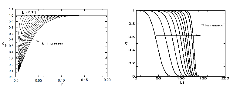
Figure 1: (a) Pole filter $g_{\phi}$ as a function of cylindrical radius $Y$ and azimuthal wavenumber $k$, with $7\leq k\leq 24$. The effects of the filter are greatest in a small region near the poles, whose cylindrical radius increases with increasing $k$. (b) Spectral filter $\sigma$ as a function of radial wavenumber $l$ (or equivalently, latitudinal wavenumber $j$) and filter order $\gamma$, with $4\leq\gamma\leq 22$. The filtering is weaker as $\gamma$ increases. The modes $k=0,\pm 1$ are not filtered, since they are important to get the correct stability characteristics. For all three wavenumbers, $g_{\phi}=1$ for all values of $Y$.

3.5 Initial and boundary conditions

3.5.1 Initial conditions for ${\bf v}_{n}$ and ${\bf v}_{s}$

The velocity fields must be divergence-free initially, in order to satisfy the incompressibility constraint (3). The easiest choice is ${\bf v}_{n}={\bf v}_{s}=0$. However, the superfluid velocity field is used to calculate the vorticity unit vector, $\mbox{\boldmath$\hat{\omega}$}_{s}$, which in turn appears in (6) and (7) and must remain well defined. Additionally, the HVBK equations describe a rotating superfluid, implying $\mbox{\boldmath$\omega$}_{s}\neq 0$ in general. A simple initial condition that satisfies $\nabla\cdot{\bf v}_{n}=\nabla\cdot{\bf v}_{s}=0$ and $\mbox{\boldmath$\omega$}_{s}\neq 0$ is the Stokes solution (Landau & Lifshitz, 1959)

$${\bf v}_{n}={\bf v}_{s}=\frac{rR_{1}^{3}R_{2}^{3}}{R_{2}^{3}-R_{1}^{3}}\left[\frac{\Omega_{1}-\Omega_{2}}{r^{3}}+\frac{\Omega_{2}}{R_{1}^{3}}-\frac{\Omega_{1}}{R_{2}^{3}}\right]\sin\theta\,{\bf e}_{\phi}.$$ (12)

This ansatz is an exact solution of the spherical Couette problem in the limit $\mbox{{Re}}\rightarrow 0$ and a respectable approximation for $\mbox{{Re}}\mathrel{\hbox to0.0pt{\lower 4.0pt\hbox{\hskip 1.0pt$\sim$}\hss}\raise 1.0pt\hbox{$<$}}10$, where meridional circulation, which is absent from (12), carries only $\sim 0.01$ % of the total kinetic energy (Dumas, 1991).

3.5.2 Boundary conditions for ${\bf v}_{n}$

The normal fluid satisfies a no-penetration condition, $({\bf v}_{n})_{r}=0$, at the inner and outer spheres. It also satisfies a no-slip condition; its tangential velocity equals that of the surface, like for a viscous, Navier-Stokes fluid. The angular velocity vector $\boldsymbol{\Omega}_{2}$, which is tilted with respect to the $z$ axis in the $x$-$z$ plane by an angle $\theta_{0}$, can be written in spherical polar coordinates as

$$\boldsymbol{\Omega}_{2} = \Omega_{2}[(\cos\theta_{0}\cos\theta+\sin\theta_{0}\sin\theta\cos\phi){\bf e}_{r}-(\cos\theta_{0}\sin\theta-\sin\theta_{0}\cos\theta\cos\phi){\bf e}_{\theta}$$

$$-\sin\theta_{0}\sin\phi{\bf e}_{\phi}],$$

while $\boldsymbol{\Omega}_{1}$ remains fixed parallel to the $z$ axis. The no-slip and no-penetration boundary conditions then reduce to

$${\bf v}_{n}(R_{1},\theta,\phi)=R_{1}\boldsymbol{\Omega}_{1}\times{\bf e}_{r},$$ (14)

$${\bf v}_{n}(R_{2},\theta,\phi)=R_{2}\boldsymbol{\Omega}_{2}\times{\bf e}_{r}.$$ (15)

3.5.3 Boundary conditions for ${\bf v}_{s}$

The distribution of quantized vorticity in the superfluid component determines the boundary conditions for ${\bf v}_{s}$. Quantized vortices in a cylindrical container are arranged in a rectilinear array parallel to the rotation axis if the rotation is slow [$\mbox{{Re}}\mathrel{\hbox to0.0pt{\lower 4.0pt\hbox{\hskip 1.0pt$\sim$}\hss}\raise 1.0pt\hbox{$<$}}268$; Barenghi & Jones (1988); Barenghi (1995)] or axisymmetric (Henderson et al., 1995; Henderson & Barenghi, 2000, 2004). Under these conditions, the numerical evolution is stable if the vortex lines are parallel to the curved wall (i.e. perfect sliding, $\boldsymbol{\omega}_{s}\times{\bf n}=0$) and perpendicular to the end plates.

In more general situations, e.g. noncylindrical containers, nonaxisymmetric flows, or fast rotation, there is no general agreement on what boundary conditions are suitable (Henderson & Barenghi, 2000). This is especially true when the rectilinear vortex array is disrupted by the Donnelly–Glaberson instability to form an isotropic, turbulent vortex tangle (Section 2.2). The radial component of the superfluid satisfies no penetration:

$$({\bf v}_{s})_{r}(R_{1},\theta,\phi)=0=({\bf v}_{s})_{r}(R_{2},\theta,\phi).$$ (16)

It is less clear how to treat the $\theta$ and $\phi$ components. Numerical solutions of the HVBK equations in cylindrical Couette geometries are stable only if there is perfect sliding at the inner and outer surfaces (Henderson et al., 1995; Henderson & Barenghi, 1995, 2004); numerical instabilities grow at rough surfaces (Henderson et al., 1995). In spherical containers, however, the vortex lines are neither perpendicular to the walls nor parallel to the rotation axis everywhere. Previous attempts to solve the HVBK equations in spherical geometries foundered partly because of these issues [Henderson & Barenghi (2004); R. Hollerbach 2004, private communication].

Khalatnikov (1965) suggested that vortex lines can either slide along, or pin to, the boundaries, or behave somewhere between these two extremes. If the boundary is not moving, the vortices terminate perpendicular to the surface (Khalatnikov, 1965). The tangential velocity ${\bf v}_{L}$ of a vortex line relative to a rough boundary moving with velocity $\bf u$ is given by (Khalatnikov, 1965; Hills & Roberts, 1977; Henderson & Barenghi, 2000)

$${\bf v}_{L}-{\bf u}=c_{1}\hat{\boldsymbol{\omega}}_{s}\times({\bf n}\times\hat{\boldsymbol{\omega}}_{s})+c_{2}{\bf n}\times\hat{\boldsymbol{\omega}}_{s},$$ (17)

where ${\bf n}$ is the unit normal to the surface, and $c_{1}$ and $c_{2}$ are coefficients describing the relative ease of sliding. The form of (17) follows from calculating the energy dissipated as vortices slip along the surface (Khalatnikov, 1965). Equation (17) is difficult to include in HVBK theory, where each fluid element is threaded by many vortex lines, because ${\bf v}_{L}$ is the velocity of a single vortex line; it cannot be calculated from ${\bf v}_{n}$ and ${\bf v}_{s}$, which are averaged over regions containing many vortex lines. Additionally, the slipping parameters $c_{1}$ and $c_{2}$ must be evaluated at each point on the surface, yet there is no experimental or theoretical study available in the literature on the precise form of these parameters. However, we can consider two simple limits of equation (17). For $c_{1}=c_{2}\rightarrow\infty$, the vortex lines slide freely along the surface and one requires

$$\boldsymbol{\omega}_{s}\times{\bf n}=0$$ (18)

in order that ${\bf v}_{L}$ remains finite; that is, the vortex lines are oriented perpendicular to the surface. On the other hand, for $c_{1}=c_{2}=0$, we have rough boundaries with ${\bf v}_{L}={\bf u}$. In spherical Couette geometries, this implies no-slip, i.e.

$${\bf v}_{s}(R_{1},\theta,\phi)=R_{1}\boldsymbol{\Omega}_{1}\times{\bf e}_{r},$$ (19)

$${\bf v}_{s}(R_{2},\theta,\phi)=R_{2}\boldsymbol{\Omega}_{2}\times{\bf e}_{r}.$$ (20)

We find empirically that conditions (19) and (3.12) lead to stable numerical evolution in most scenarios studied in this paper.

The existence of a vortex-free ($\boldsymbol{\omega}_{s}=0$) region adjacent to the boundaries, whose thickness approaches the intervortex spacing, is theoretically predicted by minimizing the free energy of a vortex array in a container (Hall, 1960; Stauffer & Fetter, 1968; Hills & Roberts, 1977; Henderson et al., 1995). However, it has not been detected conclusively in experiments (Northby & Donnelly, 1970; Mathieu et al., 1980). It is unclear how to treat this boundary layer numerically within HVBK theory, which assumes a high density of vortices, so we do not consider it further in this paper.

3.5.4 Accelerating spheres

The angular velocities of the outer and inner spheres, $\boldsymbol{\Omega}_{2}$ and $\boldsymbol{\Omega}_{1}$, can vary with time, either in a prescribed way or in reaction to the torque exerted by the fluid.

One scenario considered in this paper is free precession of the outer sphere. This situation is relevant to astrophysical systems like neutron stars (Jones & Andersson, 2002; Shaham, 1977; Link, 2003; Sedrakian, 2005) and to laboratory systems like superfluid-filled gyroscopes (Reppy, 1965). Let the outer sphere be biaxial, with symmetry axis ${\bf e}_{3}$ and constant total angular momentum ${\bf J}$, and resolve the angular velocity $\boldsymbol{\Omega}$ into components (Shaham, 1986)

$$\boldsymbol{\Omega}=\frac{{\bf J}_{\|}}{I_{\|}}+\frac{{\bf J}_{\bot}}{I_{\bot}}$$ (21)

parallel and perpendicular to the symmetry axis, with ${\bf J}={\bf J}_{\|}+{\bf J}_{\bot}$, where $I_{\|}$ and $I_{\bot}$ are the associated moments of inertia. The precession frequency $\Omega_{p}$ is then defined by

$$\boldsymbol{\Omega}_{p}={\bf J}_{\|}\displaystyle\left(\frac{1}{I_{\bot}}-\frac{1}{I_{\|}}\right)=\Omega_{p}{\bf e}_{3},$$ (22)

and the velocity of any point on the surface of the outer sphere in the inertial (lab) frame is given by

$$\frac{d{\bf x}}{dt}=R_{2}\boldsymbol{\Omega}^{\prime}\times{\bf e}_{r}-R_{2}\Omega_{p}{\bf e}_{3}\times{\bf e}_{r},$$ (23)

where $\boldsymbol{\Omega}^{\prime}=\Omega^{\prime}{\bf J}/J$ is the inertial-frame precession frequency. The back-reaction of the fluid on the container needs to be included when solving the HVBK equations self-consistently. The viscous torque accelerates (decelerates) the container. To this must be added any external torques $N_{\rm ext}$. Examples of $N_{\rm ext}$ are the electromagnetic torque on the crust of a neutron star (Ostriker & Gunn, 1969; Melatos, 1997; Spitkovsky, 2004) or the friction between a rotating container and its spindle in laboratory experiments (Tsakadze & Tsakadze, 1972, 1980). In this situation, $\boldsymbol{\Omega}_{1}$ and $\boldsymbol{\Omega}_{2}$ evolve according to

$$I_{ij}\frac{d\Omega_{j}^{1,2}}{dt}=({N}_{\rm ext}^{1,2}+{N}_{\rm int}^{1,2})_{i},$$ (24)

where $I_{ij}$ is the moment-of-inertia tensor, and $N_{\rm int}$ is the instantaneous viscous torque exerted by the normal fluid on the shell (Landau & Lifshitz, 1959),

$$N_{\rm int}^{1,2}=\frac{1}{\mbox{{Re}}}\int d\phi\int d\theta\,r\sin\theta\left(\frac{\partial v_{n\phi}}{\partial r}-\frac{v_{n\phi}}{r}\right)_{r=R_{1},R_{2}}.$$ (25)

Equation (24) is solved explicitly at each time step using a third-order Adams-Bashforth algorithm to get $\Omega_{i}(t+\Delta t)$, after advancing the flow using $\Omega_{i}(t)$ (see Section 3.2 and Appendix C.1).

4 Validation

To the best of the authors knowledge, the problem of superfluid SCF has never been solved before for $\mbox{{Re}}\gg 1$, save for an inconclusive pioneering attempt by R. Hollerbach [private communication, 2004; see also Henderson & Barenghi (2004)], who encountered numerical instabilities when implementing the cylindrical boundary conditions used by Henderson et al. (1995). Consequently, we cannot verify our code directly against previous superfluid SCF results, and we are forced into a different validation strategy: in the limit $T\rightarrow T_{c}$, the superfluid component vanishes, equation (1) reduces to the classical Navier-Stokes equation, and we validate our numerical scheme against the wealth of numerical and experimental studies available for viscous SCF.

Our three-dimensional pseudospectral HVBK solver reduces to a classical Navier–Stokes solver if all the coupling terms [HVBK friction, HVBK tension, $\nabla({\bf v}_{ns}^{2})$ and $\nu_{s}\nabla\omega_{s}$] are removed, and the ${\bf v}_{s}$ arrays are disabled. We validate our solver for three types of SCF in this regime: (i) inner sphere rotating, outer sphere stationary ($\Omega_{1}\neq 0$, $\Omega_{2}=0$); (ii) inner sphere stationary, outer sphere rotating ($\Omega_{1}=0$, $\Omega_{2}\neq 0$); and (iii) both spheres rotating ($\Omega_{1}\neq 0$, $\Omega_{2}\neq 0$). For the parameter range explored in this Section, viz. $50\leq\mbox{{Re}}_{1},\mbox{{Re}}_{2}\leq 1200$ and $0.18\leq\delta\leq 0.5$, a grid with $(N_{r},N_{\theta},N_{\phi})=(81,200,4)$ and $\Delta t=10^{-3}$ is sufficient to fully resolve the flow. A flow is regarded as fully resolved if the spectral mode amplitudes decrease quasi-monotonically with polynomial index.

The meridional streamlines drawn in the figures below correspond to the final steady state. A steady state is deemed to have been reached when the difference on the viscous torques between the inner and outer spheres satisfies $|N_{\rm ext}^{(2)}-N_{\rm int}^{(1)}|\leq 10^{-8}$. Torques are expressed in units of $\rho R_{1}^{5}\Omega_{1}^{2}$ or $\rho R_{2}^{5}\Omega_{2}^{2}$, unless otherwise indicated.

4.1 Inner sphere rotating, outer sphere stationary

Following Marcus & Tuckerman (1987a), we focus on a moderately sized gap $\delta=0.18$ with $\Omega_{1}\neq 0$ and $\Omega_{2}=0$. We look for time-dependent transitions between axisymmetric steady states characterized by zero, one, or two Taylor vortices on either side of the equatorial plane, and refer to them as $0$-, $1$-, and $2$-vortex states respectively. We obtain these basic flow states, together with an intermediate “pinched” vortex state (Bonnet & Alziary de Roquefort, 1976), as illustrated in Figures $4$, $7$ and $9$ of Marcus & Tuckerman (1987a).

Figure 2 plots the steady-state viscous inner torque (25) as a function of Reynolds number for $50\leq\mbox{{Re}}_{1}\leq 600$, normalized to the torque exerted by Stokes flow, $N_{\rm Stokes}=16\pi/[\mbox{{Re}}_{1}(1-R_{1}^{3}/R_{2}^{3})]$ (Marcus & Tuckerman, 1987a). The square symbols record the values taken from Figure $1$ of Marcus & Tuckerman (1987a), while the circles are output from our numerical code. Each point is obtained by starting from an initially stationary fluid, not the Stokes solution (12), and evolving in time until a steady state $|N_{\rm int}^{(2)}-N_{\rm ext}^{(1)}|\leq 10^{-8}$ is reached. The points obtained from our numerical simulations and the published results agree to three significant digits.

Once the basic $0$-vortex state is attained for $\mbox{{Re}}_{1}=600$, transitions to pinched, $1$-vortex, and $2$-vortex states can be induced by impulsively changing $\mbox{{Re}}_{1}$ (by reducing the viscosity) to $650$, $700$, and $900$ respectively. Below we check against Marcus & Tuckerman (1987a, b) whether our solver follows these transitions faithfully.

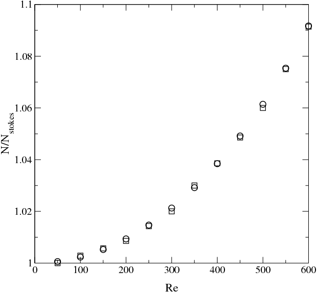
Figure 2: Viscous inner torque on the inner sphere, in units of the Stokes torque $N_{\rm Stokes}=16\pi/[\mbox{{Re}}_{1}(1-R_{1}^{3}/R_{2}^{3})]$, versus Reyolds number Re. The circles correspond to output from our numerical solver. The squares denote data taken from Marcus & Tuckerman (1987a).

4.1.1 $0\rightarrow 1$ transition

We simulate the $0\rightarrow 1$ transition by starting with a $0$-vortex equilibrium at $Re=650$ and then abruptly (over one time step) reducing the viscosity to give $Re=700$, where the equilibrum becomes unstable (Marcus & Tuckerman, 1987b). We obtain the intermediate states displayed in Figure $10$ in Marcus & Tuckerman (1987b). At the start of the sequence, the streamlines are not symmetric about the equator; the boundary between the counterrotating vortices at $t=230$ is displaced south of the equator. Then, at $t=315$, two wedges start to form in the northen hemisphere, at $\approx 82\,\deg$, and generate a growing vortex at $t=320$, which evolves into a fully developed Taylor vortex in the northen hemisphere at $t=400$. The transitions occur at about the same time as Figures $10$a–$10$b in Marcus & Tuckerman (1987b), and about $68$ units of time later than in Figures $10$c–$10$f in Marcus & Tuckerman (1987b). Figure 3 shows how the torque evolves during the time interval covered by the $0\rightarrow 1$ transition. The transition, marked by a jump in the torque, occurs later than in the numerical experiments of Marcus & Tuckerman (1987b) because it is sensitive to the exact form of the initial perturbation, which in turn depends on roundoff error, aliasing, and resolution (Marcus & Tuckerman, 1987b). The sensitivity is exacerbated by the north-south asymmetry of the $0\rightarrow 1$ transition (cf. $0\rightarrow 2$ below). However, the shapes of the solid and dashed curves in Figure 3 (especially the growth rate) agree to three significant digits if we slide them on top of each other.

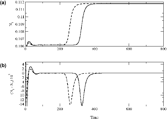
Figure 3: Torque during the $0\rightarrow 1$ transition. (a) Torque on the inner sphere, $N_{1}$, as a function of time. (b) Difference between the inner and outer torques as a function of time. The dashed curves correspond to numerical results from Marcus & Tuckerman (1987b), while the solid curves are generated by our numerical code.

4.1.2 $0\rightarrow 2$ transition

According to Marcus & Tuckerman (1987b), the $0\rightarrow 2$ transition can be produced by starting with a $0$-vortex equilibrium ($50\mathrel{\hbox to0.0pt{\lower 4.0pt\hbox{\hskip 1.0pt$\sim$}\hss}\raise 1.0pt\hbox{$<$}}\mbox{{Re}}_{1}\mathrel{\hbox to0.0pt{\lower 4.0pt\hbox{\hskip 1.0pt$\sim$}\hss}\raise 1.0pt\hbox{$<$}}651$) and impulsively increasing $\mbox{{Re}}_{1}$ above $775$, where the vortex equilibrium is unstable. We therefore start with the Stokes solution for $\mbox{{Re}}_{1}=650$ and suddenly increase $\mbox{{Re}}_{1}$ to $800$. We obtain the $0\rightarrow 2$ transitions of the meridional flow as in Figure $4$ by Marcus & Tuckerman (1987b). In Figure 4, we plot the torque on the inner sphere and the difference between the inner and outer torques as functions of time (solid curve), together with data taken from Figure $4$ of Marcus & Tuckerman (1987b) (dashed curve), showing an agreement to three significant digits, after sliding the curves together. In this case the transition is symmetric with respect to the equator and occurs more quickly. The $0\rightarrow 2$ transition is always symmetrical about the equator, as compared to the $0\rightarrow 1$ transition presented in Section 4.1.1. In a bifurcation diagram (showing the relation between torque and critical $\mbox{{Re}}_{1}$), the $0$-vortex and $2$-vortex flows lie on the same critical branch, while the $1$-vortex state lies on a different, non intersecting branch (Marcus & Tuckerman, 1987b).

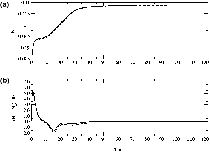
Figure 4: Torque during the $0\rightarrow 2$ transition. (a) Torque on the inner sphere, $N_{1}$, as a function of time. (b) Difference between the inner and outer torque as a function of time. The dashed curves correspond to numerical results from Marcus & Tuckerman (1987a), while the solid curves are generated by our numerical code.

4.2 Outer sphere rotating, inner sphere stationary

We now allow the outer sphere to rotate ($\Omega_{2}\neq 0$), while holding the inner sphere fixed ($\Omega_{1}=0$). We reproduce the meridional streamlines for $\mbox{{Re}}_{2}=100$, $500$, $1000$, and $2000$, with $\delta=0.5$, obtained by Dennis & Singh (1978) (Figures $3$, $4$, and $5$ of their paper), who used a numerical method in which the flow variables are expressed as a truncated series of $n$ orthogonal Gegenbauer functions with variable coefficients, reducing the Navier–Stokes equation to a set of ordinary differential equations. At $\mbox{{Re}}_{2}=500$, the agreement is good, with the streamlines showing the same distribution of vortices in the northern hemisphere: one primary circulation cell, slightly elongated in the direction of the rotation axis, with its center located $\sim 40$ deg over the equator, and a small recirculation zone near the equator. For $\mbox{{Re}}_{2}=1000$, the primary circulation cell is more elongated, with most of the circulation lying in a cylindrical sheath of radius approximately equal to $R_{1}$, as predicted by the Taylor-Proudman theorem (Pearson, 1967). For $\mbox{{Re}}_{2}=2000$, the agreement is not as good. Dennis & Singh (1978) were unable to obtain a well defined flow pattern for $\mbox{{Re}}_{2}=2000$, having been limited by computational resources to only eight Gegenbauer polynomials, which is not sufficient to follow small vortex structures developing near the equator. The higher-resolution results in our simulations suggest that the small vortices observed by Dennis & Singh (1978) near the equator are probably low-resolution artifacts.

The steady-state dimensionless torque calculated by various authors (including the present work) is presented in Table 1, together with bibliographic information.

$\mbox{{Re}}_{2}$	$N_{2}$ ($\rho R_{2}^{5}\Omega_{2}^{2}$)	Reference
$100$	$0.041745$	Present study
	$0.041750$	Dumas (1991); Dumas & Leonard (1994)
	$0.042450$	Dennis & Quartapelle (1984)
	$0.041888$	Dennis & Singh (1978)
	$0.04160$	Munson & Joseph (1971)
$500$	$0.011979$	Present study
	$0.011985$	Dumas (1991); Dumas & Leonard (1994)
	$0.012282$	Dennis & Quartapelle (1984)
	$0.011980$	Dennis & Singh (1978)
$1000$	$7.2203\times 10^{-3}$	Present study
	$7.2237\times 10^{-3}$	Dumas (1991); Dumas & Leonard (1994)
	$7.7074\times 10^{-3}$	Dennis & Quartapelle (1984)
	$7.2382\times 10^{-3}$	Dennis & Singh (1978)
$2000$	$4.4483\times 10^{-3}$	Present study
	$4.4478\times 10^{-3}$	Dennis & Singh (1978)

Table 1: Comparison of numerical values obtained by various authors for the torque on the outer sphere, $N_{2}$, when the outer sphere is rotating and the inner sphere is stationary.

4.3 Inner and outer spheres rotating

The next step in the verification program is to consider the rotation of both spheres. We follow Pearson (1967) and Munson & Joseph (1971), who studied general axisymmetric flows between rotating spheres, solving the Navier–Stokes equation in terms of stream functions in a meridional plane. Pearson (1967) used a numerical scheme based on finite differences (with typical resolution of $40\times 20$ mesh points), whereas Munson & Joseph (1971) used expansions in Legendre polynomials (typically using up to $7$ terms).

Suppose the spheres counterrotate, with $\Omega_{1}=-\Omega_{2}$. We obtatin the meridional streamlines and angular velocity profiles as shown in Figures $4$-$5$ of Munson & Joseph (1971) for $\mbox{{Re}}_{2}=100$ and $500$ respectively, with $\delta=0.5$. For $\mbox{{Re}}_{2}=100$, the agreement is good, with the $0$-vortex state rotating clockwise in the northern hemisphere, counterclockwise in the southern hemisphere, and centered at $\approx 45$ deg. The angular velocity contours are nearly concentric shells with values decreasing from $\Omega_{2}$ at the outer shell to $-\Omega_{2}$ at the inner shell. At $\mbox{{Re}}_{2}=500$, an additional counterclockwise vortex develops in the polar region, near the inner sphere, because the influence of the inner sphere strengthens as the viscosity decreases. The locations of this vortex and the main circulation cell (with its center at $\theta\approx 30$ deg) agree with the results of Munson & Joseph (1971). The angular velocity profiles show a similar pattern, forming a cylindrical sheath parallel to the rotation axes.

Now suppose that the spheres counterrotate, but with $\Omega_{1}=-2\Omega_{2}$. We do numerical simulations for $\mbox{{Re}}=\Omega_{1}R_{2}^{2}/\nu=100$ and $\mbox{{Re}}=500$ respectively. We get good agreement with the simulation results of Munson & Joseph (1971) presented in Figures $6$ and $7$ of their paper. The faster rotation of the inner sphere produces an additional circulation cell near its surface, both for $\mbox{{Re}}=100$ and $\mbox{{Re}}=500$. The center of the secondary cell is slightly displaced towards the equator in the latter case. The angular velocity contours tend to form a cylindrical sheath as the Reynolds number increases (Proudman, 1956).

Figure 5 plots the dimensionless torque as a function of the Reynolds number $\mbox{{Re}}_{1}$ or $\mbox{{Re}}_{2}$ (the definition used in each case is indicated in the plots). When the inner and outer spheres rotate in opposite directions, with $\Omega_{1}=-2\Omega_{2}$, the inner torque is shown in Figure 5a; for $\Omega_{1}=-\Omega_{2}$, the inner torque is shown in Figure 5b. When a steady state is reached, the difference between the inner and outer torques approaches $\sim 10^{-8}\rho R_{2}^{5}\Omega_{1,2}^{2}$. The solid curve and asterisks represent the data obtained by Munson & Joseph (1971) and from our numerical simulations respectively. The results coincide to three significant digits for all the Reynolds numbers considered when $\Omega_{1}=-2\Omega_{2}$. However, the results diverge for $\mbox{{Re}}\geq 500$ when $\Omega_{1}=-\Omega_{2}$. This is a consequence of the low resolution in the expansions used by Munson & Joseph (1971), who claimed to be unable to reproduce small structures near the equator, of typical size $\sim 0.3\delta$, when comparing with the study by Pearson (1967). Munson & Joseph (1971) used a maximum of $7$ modes in $r$ and $\theta$, whereas we use $N_{r}=81$ and $N_{\theta}=200$ and can therefore resolve vortical structures as small as $10^{-4}\delta$. Note that the torque is dominated by surface regions where the shear stresses are stronger, e.g. where vortices cluster.

Figure 5: (a) Dimensionless torque on the inner sphere, $c_{m}=7\mbox{{Re}}N_{1}/16\pi\rho R_{2}^{5}\Omega_{1}^{2}$, as a function of Reynolds number, Re. The spheres rotate in opposite directions, with $\Omega_{1}=-2\Omega_{2}$. (b) Dimensionless torque on the inner sphere, $c_{m}=2\mbox{{Re}}N_{1}/3\pi\rho R_{2}^{5}\Omega_{2}^{2}$ as a function of Reynolds number, Re. The spheres rotate in opposite directions, with $\Omega_{1}=-\Omega_{2}$. The solid curve corresponds to data taken from Munson & Joseph (1971). The asterisks are output from the present study.

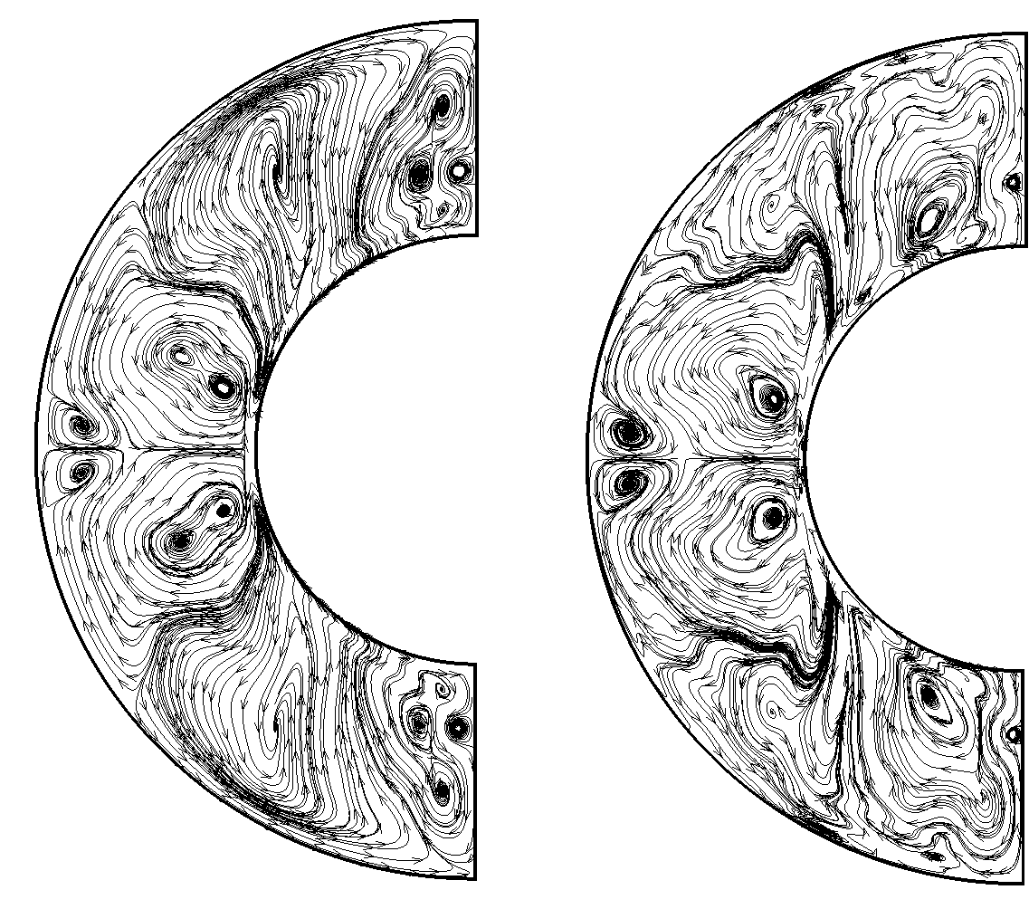
Figure 6: Snapshots at $t=214$ of meridional streamlines for the normal (left) and superfluid (right) components in superfluid SCF, with $\mbox{{Re}}=10^{4}$, $\delta=0.5$, and $\Delta\Omega=0.3$. Spectral resolution: $(N_{r},N_{\theta},N_{\phi})=(150,400,4)$. Filter parameters: $(\gamma_{r},\gamma_{\theta})=(8,6)$.

5 Unsteady, superfluid SCF

In this section, we investigate the unsteady behaviour of SCF in classical (Navier–Stokes) fluids and superfluids in two dimensions, by performing a set of axisymmetric numerical experiments ($N_{\phi}=4$) with rotational shear in the range $0.1\leq\Delta\Omega\leq 0.3$, in medium and large gaps ($0.2\leq\delta\leq 0.5$). For HV mutual friction, we use $B=1.35$ and $B^{\prime}=0.38$, the He II values at $T=1.45$ K (Barenghi et al., 1983; Donnelly, 2005; Donnelly & Barenghi, 1998). For GM mutual friction, the parameter $A^{\prime}=5.8\times 10^{-3}$ (with $\chi_{1}/\chi_{2}=0.3$) at the same temperature can be calculated from a fitting formula derived by Dimotakis (1972), which is consistent with previously published experimental values (Vinen, 1957c). Stable long-term evolution is difficult to achieve for this value of $A^{\prime}$, so we take $A^{\prime}=5.8\times 10^{-2}$ instead. We compile a preliminary gallery of vortex states, in the same spirit as for classical SCF and the validation experiments in Section 4 (Marcus & Tuckerman, 1987a, b; Dumas, 1991; Junk & Egbers, 2000); a complete classification lies outside the scope of this paper. The torque is observed to oscillate quasiperiodically, yet persistently, accompanied by oscillations in the vortical structure of the flow (Sections 5.1, 5.2). Resolution and filtering issues are discussed in Section 5.3. The role played by the inviscid superfluid, and the effect of varying the strength and form of the mutual friction force, are studied in Section 5.4 . It is observed that the superfluid tends to destabilize the flow and increases the torque. Boundary conditions are varied in Section 5.5.

5.1 Meridional streamlines

Figure 6 depicts the meridional streamlines of the normal (left) and superfluid (right) components in superfluid SCF, for the special case $\mbox{{Re}}=10^{4}$, $\delta=0.5$, and $\Delta\Omega=0.3$. In the equatorial zone ($60^{\circ}\mathrel{\hbox to0.0pt{\lower 4.0pt\hbox{\hskip 1.0pt$\sim$}\hss}\raise 1.0pt\hbox{$<$}}\theta\mathrel{\hbox to0.0pt{\lower 4.0pt\hbox{\hskip 1.0pt$\sim$}\hss}\raise 1.0pt\hbox{$<$}}120$^∘), we observe two large circulation cells adjacent to the inner boundary. Each large cell contains twin cores circulating in the same sense (and therefore tending to repel). Between the large cells and the outer boundary exist two small vortices, occupying $\approx 20$ % of the volume of the large cells. The flow in each hemisphere is symmetric about the equatorial plane. Away from the equator ($30^{\circ}\mathrel{\hbox to0.0pt{\lower 4.0pt\hbox{\hskip 1.0pt$\sim$}\hss}\raise 1.0pt\hbox{$<$}}|\theta-90^{\circ}|\mathrel{\hbox to0.0pt{\lower 4.0pt\hbox{\hskip 1.0pt$\sim$}\hss}\raise 1.0pt\hbox{$<$}}90$^∘), we observe a large cell (width $\approx 30^{\circ}$) at mid latitudes, three vortices in the normal component, and one small vortex in the superfluid component.

The flow pattern described in the previous paragraph is characteristic of moderately high Reynolds numbers ($\mbox{{Re}}\mathrel{\hbox to0.0pt{\lower 4.0pt\hbox{\hskip 1.0pt$\sim$}\hss}\raise 1.0pt\hbox{$>$}}10^{4}$). The HV mutual friction couples normal and superfluid components strongly, so that their meridional streamlines are similar. At lower Reynolds numbers ($\mbox{{Re}}\mathrel{\hbox to0.0pt{\lower 4.0pt\hbox{\hskip 1.0pt$\sim$}\hss}\raise 1.0pt\hbox{$<$}}10^{3}$), the streamlines of the two components differ markedly. The normal component behaves like a viscous, Navier–Stokes fluid at low Re, with a small number ($\mathrel{\hbox to0.0pt{\lower 4.0pt\hbox{\hskip 1.0pt$\sim$}\hss}\raise 1.0pt\hbox{$<$}}3$) of large circulation cells on each side of the equatorial plane. The superfluid is influenced less by the normal fluid, due to the stiffness provided by the vortex tension force (Henderson & Barenghi, 1995; Swanson, 1998). Streamlines of ${\bf v}_{s}$ develop multiple eddies and counter-eddies. When GM mutual friction operates, the normal and superfluid components behave similarly, both at low and high Reynolds numbers, but the superfluid displays a richer variety of circulation cells, while the normal component behaves like an uncoupled Navier–Stokes fluid. The different effects of HV and GM mutual friction are investigated in Section 5.4.

Figures 7 and 8 show the meridional streamlines at $t=20$ and $\mbox{{Re}}=3\times 10^{4}$ for the normal and superfluid components, with GM friction and zero tension force. The rotational shear $0.1\leq\Delta\Omega\leq 0.3$ increases from left to right; the dimensionless gap width $0.3\leq\delta\leq 0.5$ increases from top to bottom. The flow is approaching, but has not reached, a steady state at this time, with $|N_{\rm ext}^{(2)}-N_{\rm int}^{(1)}|\mathrel{\hbox to0.0pt{\lower 4.0pt\hbox{\hskip 1.0pt$\sim$}\hss}\raise 1.0pt\hbox{$<$}}10^{-3}$. The number for equatorial and polar circulation cells remains approximately constant as $\delta$ increases, although the cells become progressively less “stacked”. By contrast, the flow becomes less turbulent, and the number of cells decreases. Additionally, the vortices are more stacked with decreasing $\delta$.

Figures 9 and 10 show meridional streamlines at $t=14$ for the normal and superfluid components as a function of Reynolds number, for fixed $\delta$ and $\Delta\Omega$, HV friction, and nonzero tension. The streamlines of the normal fluid show the $0$-vortex state at $\mbox{{Re}}=100$ (Figure 9a). A secondary vortex develops near the outer shell at $\mbox{{Re}}=300$ (Figure 9b), whose size increases with Re, elongating in the meridional direction. Two additional vortices form in the equatorial region at $\mbox{{Re}}=10^{3}$ (Figures 9c-f). The streamlines of the superfluid component closely resemble the normal fluid component for $\mbox{{Re}}\mathrel{\hbox to0.0pt{\lower 4.0pt\hbox{\hskip 1.0pt$\sim$}\hss}\raise 1.0pt\hbox{$>$}}3\times 10^{3}$ (see Figures 10a-f).

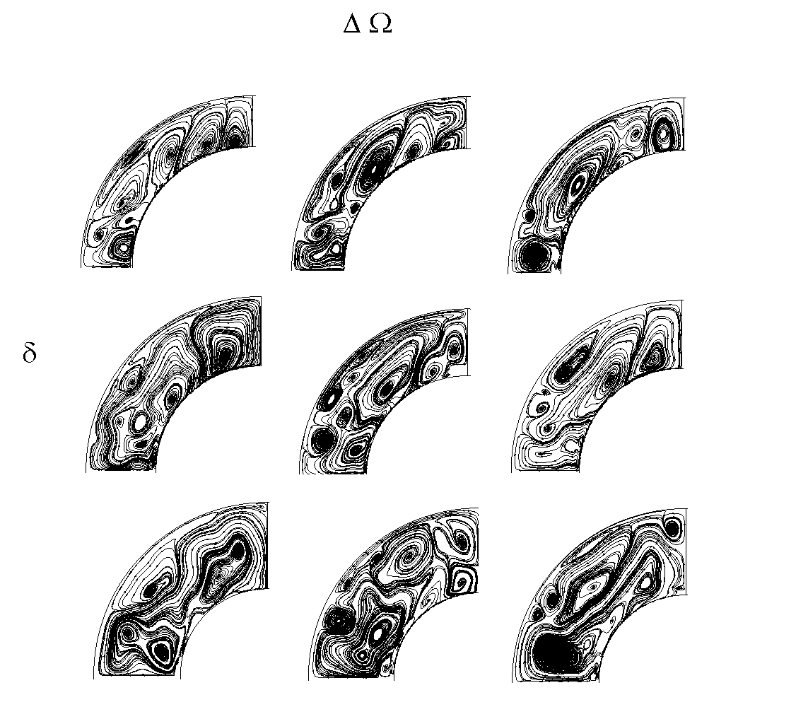
Figure 7: Snapshots at $t=20$ of meridional streamlines for the normal fluid component in superfluid SCF, with $\mbox{{Re}}=3\times 10^{4}$, $\delta=0.3$, $0.4$, $0.5$ (from top to bottom), and $\Delta\Omega=0.1$, $0.2$, $0.3$ (from left to right). The friction force if of GM form, with zero tension (${\bf T}=0$). Spectral resolution: $(N_{r},N_{\theta},N_{\phi})=(120,250,4)$. Filter parameters: $(\gamma_{r},\gamma_{\theta})=(8,8)$.

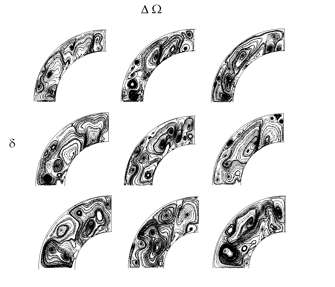
Figure 8: Snapshots at $t=20$ of meridional streamlines for the superfluid component in superfluid SCF, with $\mbox{{Re}}=3\times 10^{4}$, $\delta=0.3$, $0.4$, $0.5$ (from top to bottom), and $\Delta\Omega=0.1$, $0.2$, $0.3$ (from left to right). The friction force if of GM form, with zero tension (${\bf T}=0$). Spectral resolution: $(N_{r},N_{\theta},N_{\phi})=(120,250,4)$. Filter parameters: $(\gamma_{r},\gamma_{\theta})=(8,8)$.

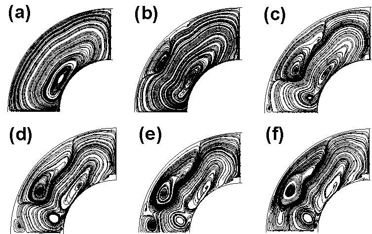
Figure 9: Snapshots at $t=14$ of meridional streamlines for the normal fluid component in superfluid SCF, with $\delta=0.5$, $\Delta\Omega=0.3$, and Re increasing from top left to bottom right. (a) $\mbox{{Re}}=100$, (b) $\mbox{{Re}}=300$, (c) $\mbox{{Re}}=1000$, (d) $\mbox{{Re}}=3000$, (e) $\mbox{{Re}}=10^{4}$, and (f) $\mbox{{Re}}=3\times 10^{4}$. The friction force is of HV form; the coefficient of the tension force is $\mbox{{Re}}_{s}=10^{-5}$. Spectral resolution: $(N_{r},N_{\theta},N_{\phi})=(120,250,4)$. Filter parameters: $(\gamma_{r},\gamma_{\theta})=(8,8)$.

Figure 10: Snapshots at $t=14$ of meridional streamlines for the superfluid component in superfluid SCF, with $\delta=0.5$, $\Delta\Omega=0.3$, and Re increasing from top to left to bottom right. (a) $\mbox{{Re}}=100$, (b) $\mbox{{Re}}=300$, (c) $\mbox{{Re}}=1000$, (d) $\mbox{{Re}}=3000$, (e) $\mbox{{Re}}=10^{4}$, and (f) $\mbox{{Re}}=3\times 10^{4}$. The friction force is of HV form; the coefficient of the tension force is $\mbox{{Re}}_{s}=10^{-5}$. Spectral resolution: $(N_{r},N_{\theta},N_{\phi})=(120,250,4)$. Filter parameters: $(\gamma_{r},\gamma_{\theta})=(8,8)$.

5.2 Unsteady torque

The torque exerted by the normal fluid component on the inner and outer spheres, calculated using (25), is plotted versus time in Figures 11a and 11b. It oscillates, with peak-to-peak amplitude $\sim 10^{-3}$ for $t\leq 30$ and $\sim 10^{-5}$ for $t\geq 30$. These oscillations, with period $\approx 2\pi/\Omega_{1}$, persist as long as the differential rotation is maintained, up to $t=214$ in our longest simulation. They are observed at all the Reynolds numbers considered in this paper ($1\times 10^{2}\leq\mbox{{Re}}\leq 3\times 10^{4}$). The oscillation amplitude is greater for HV friction; oscillations are still observed for GM friction, but with peak-to-peak amplitude $\sim 10^{-6}$. In other words, superfluid SCF is intrinsically unsteady and indeed quasiperiodic.

Figure 11: Viscous torque exerted on the (a) inner and (b) outer spheres as a function of time in superfluid SCF, with HV mutual friction, $\delta=0.5$, $\Delta\Omega=0.3$, and $\mbox{{Re}}=10^{4}$. Spectral resolution and filter parameters are the same as in Figure 6. Initially, we set ${\bf v}_{n}={\bf v}_{s}$ to the Stokes solution (12).

5.3 Spectral resolution and filter

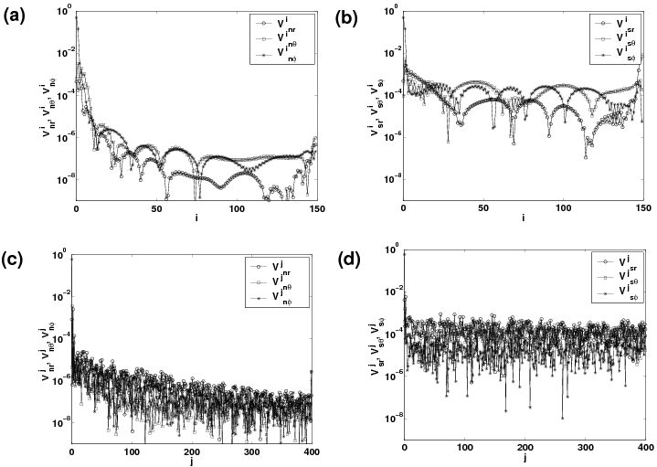
Figure 12: Snapshot of spectral mode amplitudes at $t=0.3$, as a function of the Chebyshev polynomial index $i$ for (a) the normal velocity resolutes $({\bf v}_{n})_{r}$, $({\bf v}_{n})_{\theta}$, and $({\bf v}_{n})_{\phi}$, and (b) the superfluid velocity resolutes $({\bf v}_{s})_{r}$, $({\bf v}_{s})_{\theta}$, and $({\bf v}_{s})_{\phi}$; and as a function of the sine (cosine) polynomial index $j$ for (c) the normal velocity resolutes $({\bf v}_{n})_{r}$, $({\bf v}_{n})_{\theta}$, and $({\bf v}_{n})_{\phi}$, and (d) the superfluid velocity resolutes $({\bf v}_{s})_{r}$, $({\bf v}_{s})_{\theta}$, and $({\bf v}_{s})_{\phi}$. The grid resolution is $(N_{r},N_{\theta},N_{\phi})=(150,400,4)$ and the exponential filters are switched off. Simulation parameters: HV mutual friction, $\mbox{{Re}}=178$, $\delta=0.5$, and $\Delta\Omega=0.1$.

Figure 13: Snapshot of mode amplitudes at $t=0.3$ as a function of the Chebyshev polynomial index $i$ for (a) $({\bf v}_{n})_{r}$, $({\bf v}_{n})_{\theta}$, and $({\bf v}_{n})_{\phi}$, and (b) $({\bf v}_{s})_{r}$, $({\bf v}_{s})_{\theta}$, and $({\bf v}_{s})_{\phi}$. Snapshot of mode amplitudes at $t=0.3$ as a function of the sine (cosine) polynomial index $j$ for (c) $({\bf v}_{n})_{r}$, $({\bf v}_{n})_{\theta}$, and $({\bf v}_{n})_{\phi}$, and (d) $({\bf v}_{s})_{r}$, $({\bf v}_{s})_{\theta}$, and $({\bf v}_{s})_{\phi}$. The grid resolution is $(N_{r},N_{\theta},N_{\phi})=(150,400,4)$. The exponential filter has $(\gamma_{r},\gamma_{\theta})=(8,6)$. Simulation parameters: HV mutual friction, $\mbox{{Re}}=178$, $\delta=0.5$, and $\Delta\Omega=0.1$.

In a well resolved simulation, the Chebyshev and Fourier mode amplitudes decrease monotonically (on average) with polynomial index. We prefer to maintain an amplitude ratio of at least $10^{4}$ between the strongest and weakest modes. Giacobello (2005) found empirically that this is sufficient to fully resolve vortical structures in unsteady, three-dimensional transients excited by the flow past a stationary and rotating sphere in a classical, viscous Navier–Stokes fluid. In this section, which is devoted to axisymmetric flows, we are interested in the Chebyshev ($r$) amplitudes $v^{i}_{nr,sr}$, $v^{i}_{n\theta,s\theta}$, and $v^{i}_{n\phi,s\phi}$, and Fourier ($\theta$) amplitudes $v^{j}_{nr,sr}$, $v^{j}_{n\theta,s\theta}$, and $v^{j}_{n\phi,s\phi}$. These coefficients do not correspond to $\beta_{ljk}$, $\gamma_{ljk}$, and $\delta_{ljk}$ in equations (36)–(38); $v^{i}_{nr,sr}$, $v^{i}_{n\theta,s\theta}$, and $v^{i}_{n\phi,s\phi}$ are calculated by transforming from coordinate to wavenumber space in the $r$ direction, and $v^{j}_{nr,sr}$, $v^{j}_{n\theta,s\theta}$, and $v^{j}_{n\phi,s\phi}$ are calculated by transforming from coordinate to wavenumber space in the $\theta$ direction.

We start by comparing the mode amplitudes for a poorly resolved and a well resolved simulation. Figure 12 shows an example of a poorly resolved simulation, with $\mbox{{Re}}=178$, $\delta=0.5$, $\Delta\Omega=0.1$, and $(N_{r},N_{\theta},N_{\phi})=(150,400,4)$. The spectral filter is switched off. The mode amplitudes of the normal velocity components decrease from $\sim 10^{-1}$ ($i=1$) to $\sim 10^{-6}$ ($i=150$), which superficially suggests that the flow is well resolved. However, the mode amplitudes of the superfluid velocity components are roughly constant ($\sim 10^{-4}$) across all Chebyshev ($1\leq i\leq 150$) and Fourier ($1\leq j\leq 400$) orders, indicating that the run is poorly resolved. Figure 13 shows a well resolved simulation for the same parameters. The improvement is achieved by switching on the spectral filters, and the extent of the improvement depends on the strength of the filters, with $\gamma_{r}=8$ and $\gamma_{\theta}=6$ in Figure 13. The Chebyshev amplitudes of ${\bf v}_{n}$ decrease by $\sim 8$ orders of magnitude over the index range $1\leq i\leq 25$. The Chebyshev amplitudes of ${\bf v}_{s}$ decrease more gradually, by $\sim 8$ orders of magnitude over the range $1\leq i\leq 100$. The Fourier amplitudes of ${\bf v}_{n}$ and ${\bf v}_{s}$ decay similarly (Figures 13c–d), with only $N_{\theta}\approx 20$ required to resolve the flow properly. For a weaker filter, with $\gamma_{r}=\gamma_{\theta}=12$, the mode amplitudes are unchanged to within $\sim 10$ %, but $N_{r}\approx 20$ and $N_{\theta}\approx 100$ Chebyshev and Fourier modes are required.

What happens in general when the exponential filter is either switched off, as in Figure 12, or maintained at a weak level ($\gamma_{r},\gamma_{\theta}\mathrel{\hbox to0.0pt{\lower 4.0pt\hbox{\hskip 1.0pt$\sim$}\hss}\raise 1.0pt\hbox{$>$}}20$)? For $\mbox{{Re}}\mathrel{\hbox to0.0pt{\lower 4.0pt\hbox{\hskip 1.0pt$\sim$}\hss}\raise 1.0pt\hbox{$>$}}10^{3}$, we find that the evolution is stable for a short time ($t\mathrel{\hbox to0.0pt{\lower 4.0pt\hbox{\hskip 1.0pt$\sim$}\hss}\raise 1.0pt\hbox{$<$}}10$), after which ${\bf v}_{n}$ and ${\bf v}_{s}$ become unphysically large and the numerical simulation breaks down. For $\mbox{{Re}}\sim 10^{2}$, the evolution is stable for longer, provided that perfect slip boundary conditions are applied to ${\bf v}_{s}$. Indeed, generally speaking, ${\bf v}_{s}$ evolves less stably for no-slip boundary conditions, which promote the generation of superfluid vorticity. Nevertheless, for a range of SCF parameters, we observe that ${\bf v}_{n}$ for a filtered HVBK superfluid agrees well with ${\bf v}$ for an unfiltered Navier–Stokes fluid given identical boundary conditions (see Section 5.4), engendering confidence that filtering does not cause artificial behaviour.

5.4 Effect of superfluid component

Laboratory experiments on the acceleration and deceleration of He II in spherical vessels reveal a variety of unsteady behaviour, e.g. sudden jumps and quasiperiodic oscillations in angular velocity (Tsakadze & Tsakadze, 1980). It is not known what aspects of this unsteady behaviour are caused by the nonlinear hydrodynamics of the viscous normal component of He II, or by the build-up of vorticity in the inviscid superfluid component. We now explore this question.

In order to isolate how the superfluid component influences the global dynamics of superfluid SCF, we compare three particular cases: (i) a one-component, viscous, Navier–Stokes fluid, with Reynolds number $\mbox{{Re}}=10^{4}$; (ii) a one-component, inviscid, HVBK superfluid, with ${\bf F}={\bf T}=0$ in (1) and (2); and (iii) a two-component, HVBK superfluid, whose normal component ($\mbox{{Re}}=10^{4}$) is coupled to the superfluid component through HV (Hall & Vinen, 1956a, b) and GM (Gorter & Mellink, 1949; Donnelly, 2005) mutual friction (${\bf F}\neq 0$, ${\bf T}\neq 0$). To make the comparison, we fix $\delta=0.5$ and $\Delta\Omega=0.3$.

Let us begin with case (i): a viscous, Navier–Stokes fluid. Meridional streamlines, obtained by integrating the in-plane components of the velocity field in the $x=0$ plane, are displayed in Figure 14a, at time $t=6$. The flow is complicated, featuring three primary circulation cells: one near the equator, and two near the poles (each about half the diameter of the equatorial cell). Two secondary, flattened vortices reside near the outer boundary, one just above the equator and the other centred at $r\approx 0.9$, $\theta\approx 30$^∘. These structures develop from a low-Re Stokes flow at $t=0$.

Let us repeat the experiment with an HVBK superfluid in which the normal and superfluid components are completely uncoupled, i.e. the mutual friction and tension are switched off (${\bf F}={\bf T}=0$). This is case (ii). Naturally, the normal component evolves exactly like the classical Navier–Stokes fluid in Figure 14. As for the superfluid, its meridional streamlines at time $t=6$ are shown in Figure 14b. On large scales, the flow pattern resembles Figure 14a, with the same number (three primary plus two secondary) of circulation cells. However, the cells have different shapes and diameters: the secondary cells are smaller and less flattened than in Figure 14a, and the volume of the largest (equatorial) primary cell is three times greater than in Figure 14a.

Note that equations ($1.16$) and ($1.17$) evolve independently when the coupling forces (${\bf T}$ and ${\bf F}$) are switched off. The superfluid equation of motion ($1.17$) reduces to the Euler equation for an ideal (inviscid) fluid, so only one boundary condition is required: no penetration, $({\bf v}_{s})_{r}=0$. The same is true for HV and GM mutual friction: the two forms of the friction force imply two different orders of the system of equations and hence two different sets of boundary conditions. However, there are three reasons why we do not treat HV and GM friction differently in our simulations:

1. The correct boundary conditions for the superfluid are unknown. What ultimately determines the boundary conditions for ${\bf v}_{s}$ is the distribution of quantized vorticity in the superfluid component. In cylindrical containers, it is natural to assume that the quantized vortices are arranged in a regular array parallel to the rotation axis, if the rotation is slow. Under these conditions, the numerical evolution is stable if the vortex lines are parallel to the curved wall. In spherical containers, the vortex lines are neither perpendicular to the walls nor parallel to the rotation axis everywhere. In this paper, we test what boundary conditions give the most stable evolution. Often, no slip in the superfluid component works best, even if it is not strictly mathematically correct for the GM force. Physically, we justify this by assuming that vortices pin to the boundaries, whereupon they move at the same speed. In other words, no slip corresponds to pinning at the boundaries; since we ignore the presence of the vortices in the fluid interior (${\bf T}={\bf F}=0$ at $R_{1}<r<R_{2}$) but not at the boundaries.

2. When we attempt to solve the the HVBK equations numerically with ${\bf T}=0$ in the HV friction force, or with GM friction, using only one boundary condition on the superfluid component (no penetration), the results do not differ significantly from the results presented in this paper. For $\delta=0.5$, $\Delta\Omega=0.3$, at $t=4$, the outer torque differs by $10^{-6}$ between the two approaches. One cannot see any significant difference in the streamlines of both fluids, whether one uses the strictly mathematically correct set of boundary conditions for the superfluid (no penetration only) or the simulations presented in this paper (no slip in the superfluid component).

3. The tension of the vortex lines, controlled by the stiffness parameter $\nu_{s}$, can disrupt the flow and destabilize its evolution. A high value of $\nu_{s}$ ($\mbox{{Re}}_{s}\mathrel{\hbox to0.0pt{\lower 4.0pt\hbox{\hskip 1.0pt$\sim$}\hss}\raise 1.0pt\hbox{$<$}}10^{4}$) stiffens the vortex array against the drag of the normal fluid. Previous attempts to solve the HVBK equations in spherical geometries foundered partly because of these issues. By enforcing no-slip boundary conditions on the superfluid, one ensures that the superfluid corotates with the normal fluid at the boundaries, reducing the friction force in that region. As Henderson et al. (1995) suggested (page 333, second last paragraph), the appearance of a nonlinear boundary layer may not be completely resolved by our code, or indeed by any code to date. Note also that $\nu_{s}$ is small ($\sim 10^{-5}$), so the influence of the tension term in the simulations presented in this paper is not strong. We plan to study the effects of the tension force in a future paper, when we are able to obtain a better understanding of the nonlinear boundary layer.

When the mutual friction and tension forces are switched on, as in case (iii), the vortical structures near the poles change. Consider first what happens when ${\bf F}$ is of HV form. For the normal fluid component, displayed in Figure 14c, the flattened vortex near the pole widens radially to about twice the size of the same vortex with ${\bf F}=0$, while its latitudinal extent remains unchanged. The vortex near the equator halves in size, compared to its counterpart in Figure 14a. The only appreciable changes in the superfluid flow pattern, displayed in Figure 14d, are the following: (i) the small vortex near the pole widens radially by $\sim 10$ %; and (ii) the larger circulation cell near the pole comes to resemble the same cell in the normal component more closely.

By contrast, when ${\bf F}$ is of GM form, the streamlines of the normal fluid are very similar to a classical viscous fluid at the same Reynolds number, as we can appreciate by comparing Figures 14a and 14e. The superfluid component closely resembles an uncoupled superfluid (c.f. Figures 14b and 14f). The two components are loosely coupled because GM friction is weaker than HV friction [$|{\bf F}_{\rm HV}/{\bf F}_{\rm GM}|\sim 10^{5}$; see Peralta et al. (2005, 2006b)].

Figure 14: Meridional streamlines in SCF for (a) viscous Navier–Stokes fluid with $\mbox{{Re}}=10^{4}$, (b) pure one-component inviscid superfluid, (c) normal fluid component of an HVBK superfluid with HV friction, (d) superfluid component of an HVBK superfluid with HV friction, (e) normal fluid component with GM friction, and (f) superfluid component with GM friction. All snapshots are taken at $t=6$. SCF parameters: $\delta=0.5$ and $\Delta\Omega=0.3$.

The evolution of the torque on the inner and outer spheres is plotted in Figure 15 for cases (i) and (iii). [The torque is zero in case (ii), where the fluid is completely inviscid.] The solid curve corresponds to a viscous, Navier–Stokes fluid, while the dashed and dotted curves correspond to an HVBK superfluid with HV and GM mutual friction respectively. Note that, in an HVBK superfluid, the torque is still exerted by viscous stresses in the normal component. However, its magnitude is modified by the presence of the superfluid component, because the mutual friction modifies ${\bf v}_{n}$ and hence $\partial({\bf v}_{n})_{i}/\partial x_{j}$.

The torque exerted by the normal component increases roughly thrice relative to case (i) when the superfluid component is included with HV mutual friction. By contrast, the torques exerted by a Navier–Stokes fluid and a HVBK superfluid with GM mutual friction differ by $6$ %, which is barely distinguishable on the scale of Figure 15. To understand this effect quantitatively, consider the streamline snapshots of the Navier–Stokes fluid, viscous HVBK component, and inviscid HVBK component at $t=20$, shown in Figures 16a–16c. There are four circulation cells near the outer boundary in the Navier–Stokes fluid and six in the normal HVBK component. The magnitude of the torque increases with the number of circulation cells, because more circulation cells imply steeper radial velocity gradients. We observe this in the quantity $dN_{1,2}/d(\cos\theta)$, which measures the differential contribution to the torque as a function of colatitude and is plotted in Figure 17 for the inner and outer spheres. For example, we find $|dN_{1}/d(\cos\theta)|<0.1$ for the Navier–Stokes fluid, but $|dN_{1}/d(\cos\theta)|$ is as large as $0.5$ (at $\theta\approx 75^{\circ}$, $110^{\circ}$) for the HVBK superfluid with HV mutual friction. From equation (25), we see that $N_{1}$ and $N_{2}$ in the HVBK superfluid are greater due to larger contributions from the first term in (25), viz. $\partial v_{n\phi}/\partial r$. For example, at $r=R_{2}$ and $\theta\approx 45^{\circ}$, we find $\partial v_{\phi}/{\partial r}\approx-0.73$ for the Navier–Stokes fluid and $(\partial v_{n\phi}/{\partial r})\approx-3.46$ for the normal component of the HVBK superfluid, whereas the second term in (25) is similar in both systems, viz. $v_{n\phi}/r\approx v_{\phi}/r\approx 0.49$.

Behaviour of the sort just described was predicted by Henderson & Barenghi (1995), who solved the HVBK equations numerically inside infinitely long, differentially rotating cylinders. They too observed that, as Re increases, the tension force diminishes, and the friction force dominates. Inside the circulation cells of the normal fluid, the ratio $|{\bf T}|/|{\bf F}_{\rm HV}|$ decreases with increasing Re. Henderson & Barenghi (1995) suggested that, at higher Re, the mutual friction locks together ${\bf v}_{n}$ and ${\bf v}_{s}$, so that the streamlines of the superfluid and normal fluid are similar.

In order to quantify how the two-fluid coupling changes with Re, consider a HVBK superfluid with the same parameters as in Figure 16b and 16c, but with $\mbox{{Re}}=178$ instead of $\mbox{{Re}}=10^{4}$. Figure 18 compares a sequence of snapshots of the meridional streamlines for $\mbox{{Re}}=178$ and $10^{4}$ at times $10\leq t\leq 60$. For $\mbox{{Re}}=178$, the normal component differs markedly from the superfluid component, except during the early stages of the evolution ($t\leq 10$). Eventually, at $t\geq 30$, the normal fluid settles down into a permanent $0$-vortex state, while the superfluid develops $3$–$4$ vortices near the equator. For $\mbox{{Re}}=10^{4}$, on the other hand, the normal and superfluid components display similar flow patterns, with the same number of vortices in approximately the same locations. This occurs because the HV mutual friction progressively dominates the vortex tension as Re increases and also as time passes. Quantitative evidence is presented in Figure 19, where $|{\bf T}|/|{\bf F}_{\rm HV}|$ is plotted as a function of colatitude in the equatorial region $80^{\circ}\leq\theta\leq 100^{\circ}$, at the boundary of the outer sphere ($r=R_{2}$). However, this initial transient soon disappears, and the inequality reverses. At $t=10$, we find $(|{\bf T}|/|{\bf F}_{\rm HV}|)_{\mbox{{Re}}=178}<(|{\bf T}|/|{\bf F}_{\rm HV}|)_{\mbox{{Re}}=10^{4}}$ except at $\theta\approx 85^{\circ}$ and $\theta\approx 95^{\circ}$ (see Figure 19a). At $t=20$, we find $(|{\bf T}|/|{\bf F}_{\rm HV}|)_{\mbox{{Re}}=178}>(|{\bf T}|/|{\bf F}_{\rm HV}|)_{\mbox{{Re}}=10^{4}}$, except in the narrow region $87^{\circ}\mathrel{\hbox to0.0pt{\lower 4.0pt\hbox{\hskip 1.0pt$\sim$}\hss}\raise 1.0pt\hbox{$<$}}\theta\mathrel{\hbox to0.0pt{\lower 4.0pt\hbox{\hskip 1.0pt$\sim$}\hss}\raise 1.0pt\hbox{$<$}}93^{\circ}$. For $t\geq 30$, we find $(|{\bf T}|/|{\bf F}_{\rm HV}|)_{\mbox{{Re}}=178}>(|{\bf T}|/|{\bf F}_{\rm HV}|)_{\mbox{{Re}}=10^{4}}$ throughout the equatorial region $80^{\circ}\leq\theta\leq 100^{\circ}$ (except for a brief reversal at $t\approx 50$). Thus, at low Reynolds numbers ($\mbox{{Re}}\mathrel{\hbox to0.0pt{\lower 4.0pt\hbox{\hskip 1.0pt$\sim$}\hss}\raise 1.0pt\hbox{$<$}}10^{3}$) and at early times, the tension force dominates the mutual friction throughout most of the fluid, while the opposite is true at high Reynolds numbers and late times. The stiffness of the superfluid vortex array, encoded in the tension force, prevents ${\bf v}_{s}$ from following ${\bf v}_{n}$, whereas, when the mutual friction dominates, ${\bf v}_{s}$ copies ${\bf v}_{n}$ more closely.

As the tension is less important at higher Re, one expects the superfluid component to influence the overall dynamics less as Re increases. This is reflected in the torque. For a viscous fluid at $\mbox{{Re}}=178$, the torque is half that for a superfluid at the same Reynolds number. For a superfluid with $\mbox{{Re}}=10^{4}$, the torque doubles when compared with a viscous fluid with the same Reynolds number. In Section 5.5, we quantify how the boundary condition on the superfluid component (indirectly) affects the torque.

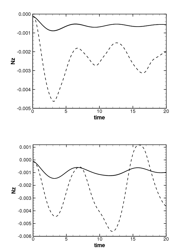
Figure 15: Torque on the inner (upper plot) and outer (lower plot) spheres, for a viscous fluid (solid curve), a superfluid with HV mutual friction force (dashed curve), and a superfluid with GM mutual friction (dotted curve). In all cases, we take $\mbox{{Re}}=10^{4}$, $\delta=0.5$, and $\Delta\Omega=0.3$. The solid and dotted curves differ by one part in $10^{4}$, and are almost indistinguishable on the scale of the plot.

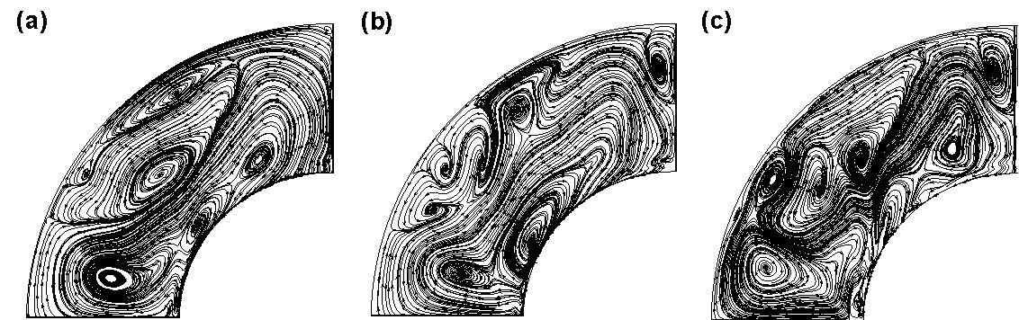
Figure 16: Meridional streamlines in SCF for (a) viscous Navier–Stokes fluid, (b) normal fluid component, with HV mutual friction, and (c) superfluid component with HV mutual friction, with $\mbox{{Re}}=10^{4}$. All snapshots are taken at $t=20$. SCF parameters: $\delta=0.5$ and $\Delta\Omega=0.3$.

Figure 17: Differential torque $dN_{z}/d(\cos\theta)$ as a function of colatitude $\theta$ for the inner (upper plot) and outer (lower plot) spheres, for a viscous Navier–Stokes fluid (solid curve), a superfluid with HV mutual friction (dashed curve), and a superfluid with GM mutual friction (dotted curve), at time $t=20$. SCF parameters: $\mbox{{Re}}=10^{4}$, $\delta=0.5$, and $\Delta\Omega=0.3$.

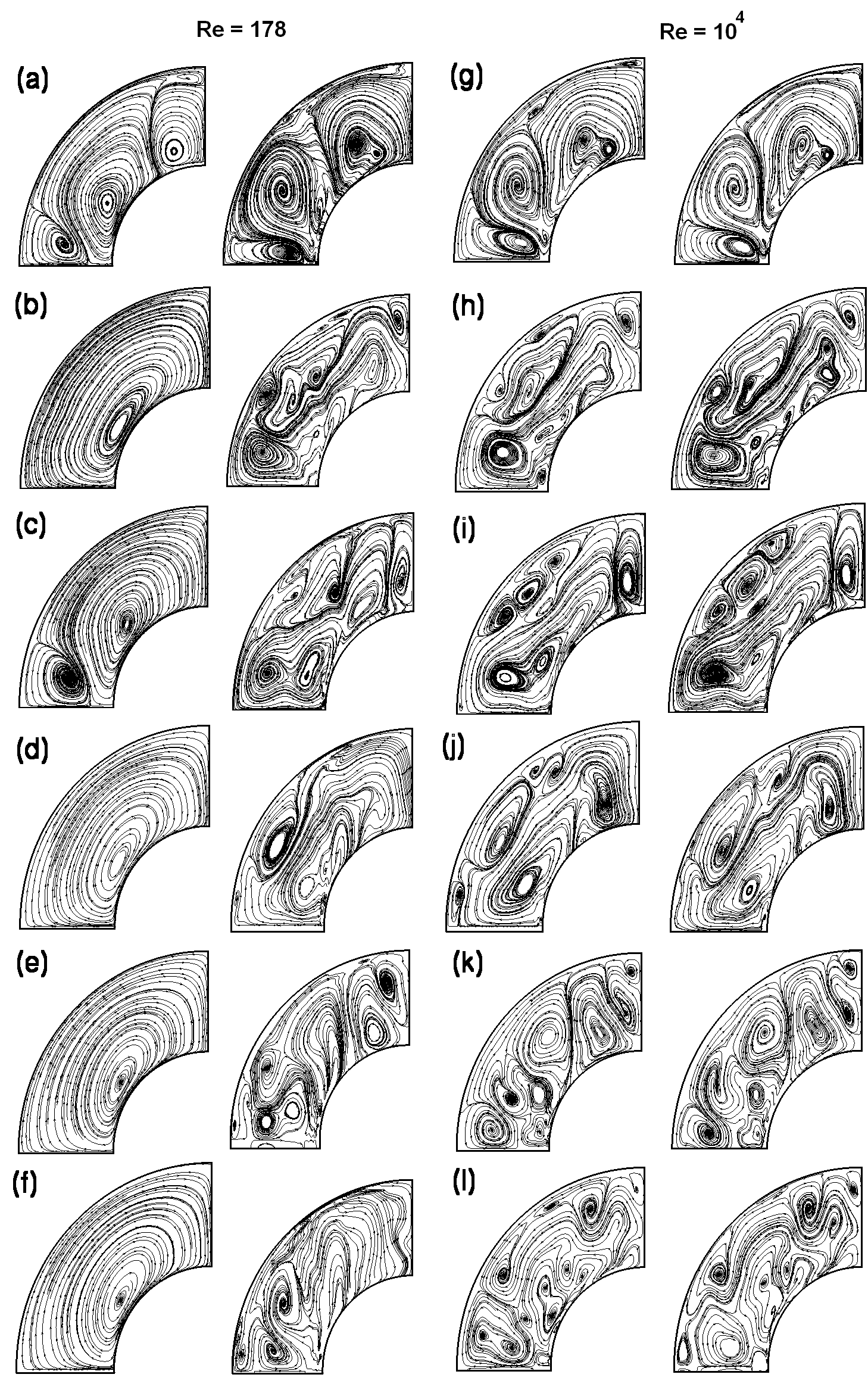
Figure 18: Meridional streamlines in superfluid SCF at low and high Reynolds numbers. Left half of figure: $\mbox{{Re}}=178$, at times (a) $t=10$, (b) $t=20$, (c) $t=30$, (d) $t=40$, (e) $t=50$, and (f) $t=60$. Right half of figure: $\mbox{{Re}}=10^{4}$, at times (g) $t=10$, (h) $t=20$, (i) $t=30$, (j) $t=40$, (k) $t=50$, and (l) $t=60$. In each snapshot, the left-hand and right-hand quadrants display the normal and superfluid components respectively. SCF parameters: $\delta=0.5$, $\Delta\Omega=0.3$, and $\mbox{{Re}}_{s}=10^{5}$.

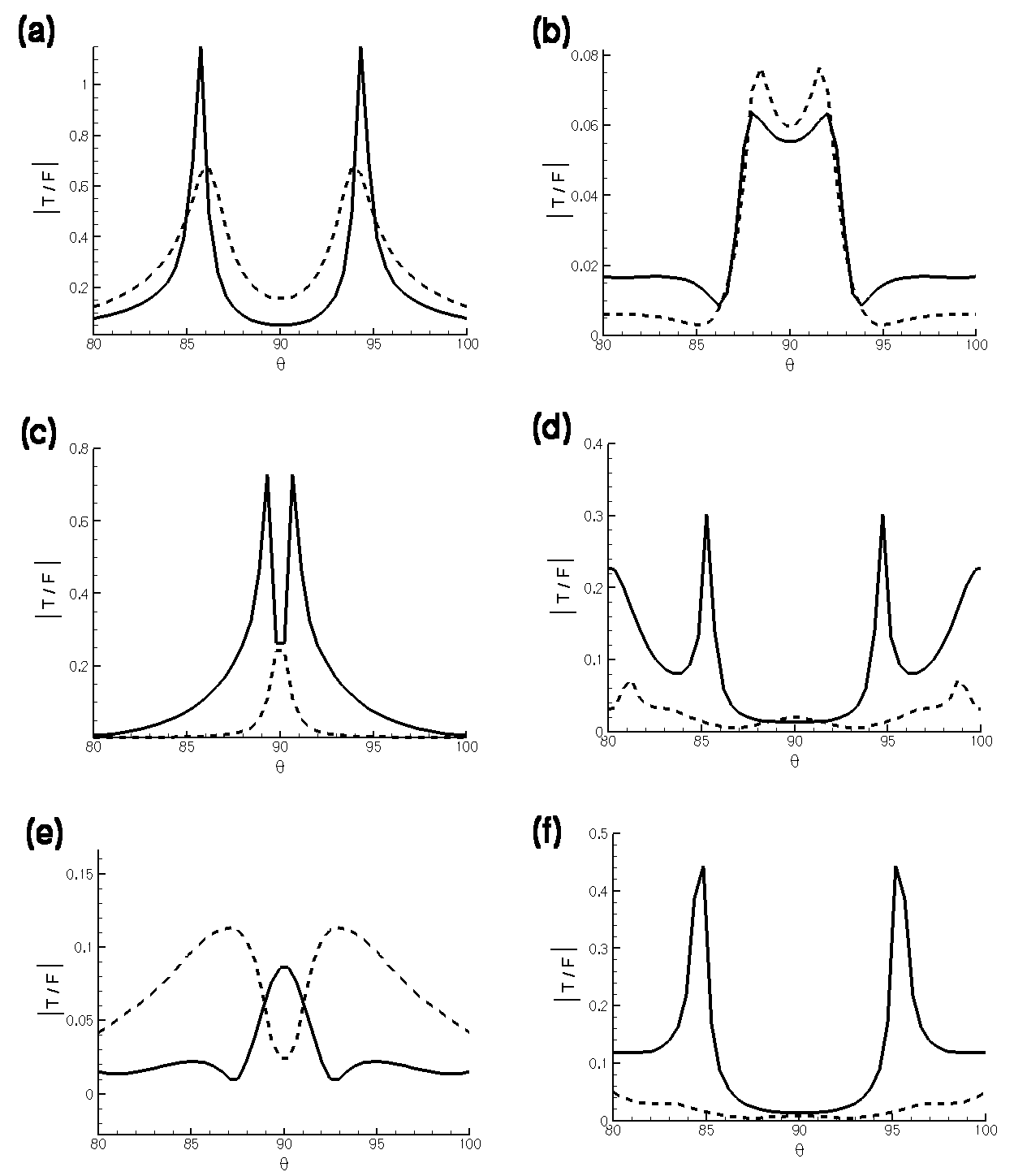
Figure 19: Ratio of the tension force $({\bf T})$ to the HV mutual friction force $({\bf F}_{\rm HV})$ as a function of colatitude $\theta$ (in ^∘), at the boundary of the outer sphere, at times (a) $t=10$, (b) $t=20$, (c) $t=30$, (d) $t=40$, (e) $t=50$, and (f) $t=60$. SCF parameters: $\delta=0.5$, $\Delta\Omega=0.3$, $\mbox{{Re}}=178$ (solid curve), and $\mbox{{Re}}=10^{4}$ (dashed curve). Generally speaking, $|{\bf T}|/|{\bf F}_{\rm HV}|$ decreases with Re and $t$.

5.5 Effect of the boundary conditions

The streamlines of the normal and superfluid components resemble each other ever more closely as Re increases, suggesting that the frictional coupling is responsible, as argued in Section 5.4. Nevertheless, it is important to check how much of the similarity arises from imposing the no-slip boundary condition on the superfluid component at $r=R_{1}$, $R_{2}$, which in turn imposes zero counterflow (${\bf v}_{n}={\bf v}_{s}$) at $r=R_{1}$, $R_{2}$. This matters, because it can be argued that the no-slip condition is artificial. The physically correct boundary conditions on ${\bf v}_{s}$ are still uncertain, lying somewhere between the following two extremes: (i) quantized vortex lines slide freely along the surface, thereby terminating perpendicular to it, as expressed by (19); or (ii) quantized vortices are pinned to the surface, so that ${\bf v}_{s}$ does not slip relative to the surface, as expressed by (18) (Khalatnikov, 1965).

To clarify these matters, we repeat two of the no-slip simulations in Section 5.4 (with $\mbox{{Re}}=178$ and $\mbox{{Re}}=10^{4}$, as well as $\delta=0.5$ and $\Delta\Omega=0.3$) such that the superfluid satisfies the perfect-slip boundary condition (18) instead of the no-slip condition (19). Perfect slip implies that the vortex lines terminate perpendicular to the surfaces of the inner and outer spheres. The normal fluid satisfies the no-slip condition (14). Both ${\bf v}_{n}$ and ${\bf v}_{s}$ are initialized to the Stokes solution (12).

Figure 20 compares the results for no slip and perfect slip at $t=18$. For both low ($\mbox{{Re}}=178$) and high ($\mbox{{Re}}=10^{4}$) Reynolds numbers, the large-scale structure of the flow is the same under both kinds of boundary conditions. For example, in both Figures 20a (perfect slip) and 20b (no slip), ${\bf v}_{s}$ exhibits three large circulation cells: one near the pole, centered near the inner sphere, at $\theta\approx 30$ and $r\approx 0.6$; one at mid-latitudes, centered near the outer sphere, at $\theta\approx 45^{\circ}$ and $r\approx 0.8$; and one at the equator, whose diamater is half that of the polar cell. Similar structures are also observed at $\mbox{{Re}}=10^{4}$ in Figures 20c (perfect slip) and 20d (no slip). On the other hand, the detailed internal structure of the cells does depend on the type of boundary condition employed, expecially at lower Re. For example, when there is no slip, the centers of the circulation cells develop additional small vortices, and the streamlines at $r=R_{1}$, $R_{2}$ become jagged.

In conclusion, therefore, the global resemblance of the ${\bf v}_{n}$ and ${\bf v}_{s}$ streamlines at high Re found in Section 5.4 is not an artifact of imposing no slip on ${\bf v}_{s}$ at the boundaries. It is observed equally when perfect slip is allowed. Indeed, the choice of boundary conditions affects the ${\bf v}_{s}$ flow pattern only as far as the small-scale structure in the cell cores is concerned. (Of course, the ${\bf v}_{n}$ streamlines are almost independent of the boundary condition used for the superfluid.) If HV mutual friction is replaced by (weaker) GM mutual friction, the resemblance lessens, with ${\bf v}_{n}$ tending to look like a Navier–Stokes flow (Figure 14a) and ${\bf v}_{s}$ tending to look like an uncoupled superfluid (Figure 14b).

The torque on the outer and inner spheres is plotted versus time in Figures 21a–21b, for perfect slip (solid curve) and no slip (dashed curve). A viscous Navier–Stokes fluid is also plotted for comparison (dotted curve). The perfect-slip boundary condition on ${\bf v}_{s}$ roughly halves the amplitude of the torque compared to the no-slip boundary condition.

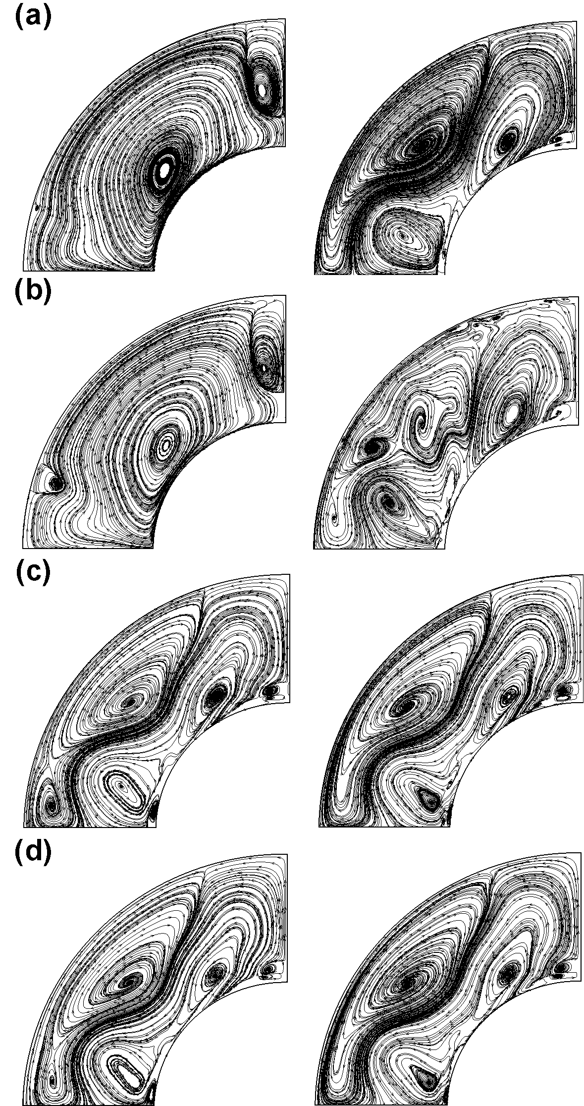
Figure 20: Meridional streamlines in superfluid SCF for the normal (left panels) and superfluid (right panels) components, at time $t=18$, for $\delta=0.5$, $\Delta\Omega=0.3$, and $\mbox{{Re}}_{s}=10^{5}$. The panels illustrate the effect of boundary conditions. (a) $\mbox{{Re}}=178$, perfect-slip boundary condition (18) on ${\bf v}_{s}$; (b) $\mbox{{Re}}=178$, no-slip boundary condition (19) on ${\bf v}_{s}$; (c) $\mbox{{Re}}=10^{4}$, perfect-slip boundary condition (18) ; and (d) $\mbox{{Re}}=10^{4}$, no-slip boundary condition.

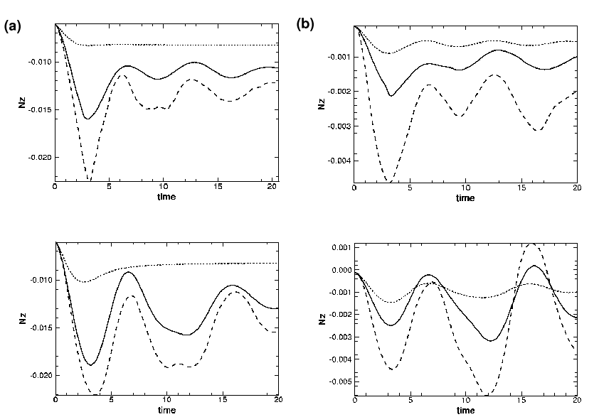
Figure 21: Evolution of the inner torque (upper plots) and outer torque (lower plots) for superfluid SCF with $\delta=0.5$, $\Delta\Omega=0.3$, and Reynolds number (a) $\mbox{{Re}}=178$ and (b) $\mbox{{Re}}=10^{4}$. The solid, dashed, and dotted curves correspond to an HVBK superfluid with perfect-slip boundary condition on ${\bf v}_{s}$, an HVBK superfluid with no-slip boundary condition on ${\bf v}_{s}$, and a viscous Navier–Stokes fluid, respectively.

6 Nonaxisymmetric spherical Couette flow

We take advantage of the three-dimensional capabilities of our numerical solver to investigate two systems that exhibit nonaxisymmetric flow (requiring spectral resolution $N_{\phi}\mathrel{\hbox to0.0pt{\lower 4.0pt\hbox{\hskip 1.0pt$\sim$}\hss}\raise 1.0pt\hbox{$>$}}12$): (i) a spherical, differentially rotating shell in which the rotation axes of the inner and outer spheres are mutually inclined; and (ii) a spherical, differentially rotating shell in which the outer sphere precesses freely, while the inner sphere rotates uniformly or is at rest. These systems have never been studied before. We use standard vortex identification methods, introduced by Chong et al. (1990) in viscous flows, to fully characterize the three-dimensional vortex structures we encounter — the first time this has been done for an HVBK superfluid. One incidental outcome of the work is to confirm that our numerical method can resolve fine structures in superfluid flow.

6.1 Characterizing the flow topology

To understand the topology of a three-dimensional flow, one must classify the vortices it contains. In its simplest guise, a vortex coincides with a local pressure minimum, where the centrifugal acceleration balances the radial pressure gradient. However, this criterion fails in situations where unsteady strains or viscous effects (at low Reynolds numbers) balance the centrifugal force (Chong et al., 1990; Jeong & Hussain, 1995). A second simplistic approach is to use $|\boldsymbol{\omega}|=|\nabla\times{\bf v}|$ to identify local concentrations of vorticity (Metcalfe et al., 1985). However, this method can lead to confusion in wall-bounded flows, like ours, where the vorticity produced by a wall-driven background shear can mask the main vortical structures of the flow, and one needs to know the location of the vortex core beforehand (Robinson, 1991).

Several sophisticated alternatives to the simple pressure minimum and vorticity magnitude tests have been developed. Most are based on invariants of the velocity gradient tensor (Hunt et al., 1988). We describe two tests below: the discriminant definition of a vortex, which is insensitive to numerical error, especially in Couette geometries (Frana et al., 2005); and the $\lambda_{2}$ definition, which is suited better to open geometries, e.g. the flow past a rotating sphere (Giacobello, 2005).

6.1.1 Discriminant definition of a vortex

The velocity gradient tensor $A_{ij}=\partial v_{i}/\partial x_{j}$ measured by a nonrotating observer that moves locally with the fluid can be decomposed into a symmetric ($S_{ij}$, or rate-of-strain tensor) and an antisymmetric ($W_{ij}$, or rate-of-rotation tensor) part:

$$A_{ij}=S_{ij}+W_{ij}=\frac{1}{2}\left(\frac{\partial v_{i}}{\partial x_{j}}+\frac{\partial v_{j}}{\partial x_{i}}\right)+\frac{1}{2}\left(\frac{\partial v_{i}}{\partial x_{j}}-\frac{\partial v_{j}}{\partial x_{i}}\right).$$ (26)

The eigenvalues $\lambda$ are roots of the characteristic polynomial $\lambda^{3}+P_{A}\lambda^{2}+Q_{A}\lambda+R_{A}=0$, whose coefficients are defined by

$$P_{A} = -{\rm tr}(A_{ij})=-S_{ii},$$ (27)

$$Q_{A} = \frac{1}{2}[P_{A}^{2}-{\rm tr}(A_{ij}^{2})]=\frac{1}{2}(P_{A}^{2}-S_{ij}S_{ji}-W_{ij}W_{ji}),$$ (28)

$$R_{A} = -{\rm det}(A_{ij})=\frac{1}{2}(-P_{A}^{3}+3P_{A}Q_{A}-S_{ij}S_{jk}S_{ki}-3W_{ij}W_{jk}W_{ki}).$$ (29)

These quantities are invariant under any nonrotating coordinate transformation. The quantity $P_{A}$ is the trace of the velocity gradient tensor (that is, the continuity equation); in an incompressible fluid, one has $P_{A}=0$. The quantity $Q_{A}$ measures the excess of rotation over strain. The sign of $R_{A}$ governs the stability of the flow (see below). The scalar invariants $R_{A}$ and $Q_{A}$ can be combined to form the discriminant $D_{A}=Q_{A}^{3}+27R_{A}^{2}/4$ (Soria & Cantwell, 1994).

• If $D_{A}>0$ at some point in the flow, $A_{ij}$ at that point has one real and two complex conjugate eigenvalues. Following the nomenclature of Chong et al. (1990), we say that such points are focal in nature. Streamlines wrap around the axis of the real eigenvector and describe a spiral in the plane spanned by the two complex eigenvectors. The sense of the spiral is determined by the sign of $R_{A}$. For $R_{A}>0$, the trajectories are attracted towards the axis of the real eigenvector; the point is an unstable focus/contracting (UF/C) (Chong et al., 1990). For $R_{A}<0$, the trajectories are repelled away from the eigenvector; the point is a stable focus/stretching (SF/S).

• If $D_{A}<0$, all the eigenvalues are real. We say that such points are strain dominated (Soria & Cantwell, 1994). Streamlines either approach or flee the point along the three independent, intersecting, real eigenvectors. When projected onto the three planes spanned by the eigenvectors, the trajectories asymptotically approach the eigenvector axes along “parabola-like” or “hyperbola-like” paths, depending on the sign of $R_{A}$. If $R_{A}<0$, we get a stable node/saddle/saddle (SN/S/S); if $R_{A}>0$, we get an unstable/node/saddle/saddle (UN/S/S). The degenerate case $R_{A}=0$ corresponds to a two-dimensional flow.

In this paper, we plot topological isosurfaces according to the following colour scheme. Regions with $D_{A}>0$ which are SF/S and UF/C are coloured yellow and light blue respectively. Regions with $D_{A}<0$ which are SN/S/S and UN/S/S are coloured orange and green respectively.

6.1.2 $\lambda_{2}$ definition of a vortex

Jeong & Hussain (1995) realized that the existence of a pressure minimum is not a sufficient and necessary condition for a vortex core to be present. For example, an unsteady flow can create a pressure minimum even where there is no vortex. On the other hand, centrifugal forces can cancel viscous forces perfectly (e.g. Kármán’s viscous flow, or a Stokes flow at low Re), thereby eliminating a pressure minimum even though a vortex is present (Jeong & Hussain, 1995).

The $\lambda_{2}$ criterion seeks to locate the pressure minimum in a plane perpendicular to the vortex axis by eliminating unsteady strains and viscous stresses from the Navier–Stokes equations. Decomposing $A_{ij}$ into symmetric and anti-symmetric parts and substituting into the Navier–Stokes equation, we obtain, for the symmetric part,

$$\frac{\partial S_{ij}}{\partial t}+v_{k}\frac{\partial S_{ij}}{\partial x_{k}}-\frac{1}{\mbox{{Re}}}\frac{\partial^{2}S_{ij}}{\partial x_{k}\partial x_{k}}+S_{kj}S_{ik}+W_{kj}W_{ik}=-\frac{\partial^{2}p}{\partial x_{i}\partial x_{j}}.$$ (30)

The Hessian of the pressure, $\partial^{2}p/{\partial x_{i}\partial x_{j}}$, contains information about pressure minima. The existence of a pressure minimum requires the Hessian to have two positive eigenvalues (Jeong & Hussain, 1995). Ignoring the unsteady strain [first term in (30)] and the viscous stress [third term in (30)], a vortex is defined as a connected region with two negative eigenvalues of the tensor ${\bf S}^{2}+{\bf W}^{2}$, which is symmetric and has real eigenvalues only. Hence, if we call the eigenvalues $\lambda_{1}$, $\lambda_{2}$, and $\lambda_{3}$ and order them such that $\lambda_{1}\geq\lambda_{2}\geq\lambda_{3}$, we define a vortex to be a region where one has $\lambda_{2}<0$ (Jeong & Hussain, 1995).

6.2 Misaligned spheres

In this section, we consider a spherical shell filled with superfluid ($\delta=0.3$, $\mbox{{Re}}=10^{3}$ or $10^{4}$), whose inner and outer surfaces rotate at the same angular speed, $\Omega_{1}=\Omega_{2}=1.0$, but about different rotation axes. The outer sphere rotates about an axis inclined with respect to the $z$ axis, in the $x$-$z$ plane, by an angle $\theta_{0}=3$^∘, while the inner sphere rotates about the $z$ axis. We present a gallery of some of the flows excited in this system and characterize their topologies employing the methods in Section 6.1. Our results are merely a first attempt at this problem; a lot remains to be learnt about the nonlinear physics behind such flows.

No-slip boundary conditions (14) are imposed on ${\bf v}_{n}$, while the superfluid satisfies either perfect slip (19) or no slip (18). The mutual friction takes the GM form (8). We fail to obtain stable evolution for HV mutual friction (6) or large inclination angles ($\theta_{0}\geq 3^{\circ}$); the simulation becomes unresolved in $\phi$ unless $N_{\phi}\geq 20$ is used, straining our computing budget.

6.2.1 Topology of the flow

Investigations of the flow past a sphere (Giacobello, 2005) found that the $\lambda_{2}$ criterion is better at identifying nonaxisymmetric vortex structures than the discriminant criterion, validating the findings of Jeong & Hussain (1995), who noticed that vortical structures identified using $D_{A}$ tend to have noisy boundaries. Recently, however, investigations of Taylor-Görtler vortices in cylindrical containers by Frana et al. (2005) revealed that the vortex contours identified by the $\lambda_{2}$ criterion can be severely perturbed by numerical noise, unlike the discriminant criterion. We find this too. The discriminant criterion is better suited to enclosed geometries than the $\lambda_{2}$ criterion, while the opposite is true for open geometries.

In Figures 22a–c, we plot isosurfaces of $\lambda_{2}$ ($\lambda_{2}=-0.5$, $-1$, $-3$) for the normal component in superfluid SCF with $\mbox{{Re}}=10^{3}$, at $t=50$. It is hard to discern the regions of the flow which are vorticity dominated. Moreover, when varying the isosurface from $\lambda_{2}=-0.5$ to $\lambda_{2}=-3$, we find that its overall shape changes greatly, which is undesirable; the visualization method should be insensitive to the threshold (Giacobello, 2005). By contrast, when we use the discriminant criterion, as in Figures 22d–f, focal regions in ${\bf v}_{n}$ are cleary visible, and their shape is preserved despite varying the threshold over four decades ($10^{-4}\leq D_{A}\leq 1$).

The discriminant criterion allows us to diagnose the topology of the inviscid superfluid component as well. In Figure 23, we present isosurfaces of $D_{A}=10^{-4}$ (Figures 23a–d) and $D_{A}=-10^{-4}$ (Figures 23e–h) for ${\bf v}_{s}$ in superfluid SCF with $\mbox{{Re}}=10^{3}$ and no-slip boundary conditions on ${\bf v}_{s}$. Throughout most of the volume, the flow is focal, or vorticity-dominated. Strain-dominated regions, shown in orange, also exist, but are less widespread. They have a threaded structure (Figures 23e–h), which is maintained when we increase the Reynolds number to $\mbox{{Re}}=10^{4}$, because ${\bf v}_{s}$ is weakly coupled to ${\bf v}_{n}$ via GM mutual friction (see Section 5.4). Perfect-slip boundary conditions on ${\bf v}_{s}$ do not alter the topology. The normal fluid dynamics, on the other hand, is almost completely dominated by vorticity, as Figures 24a–d show. Strain-dominated regions are only detected in small regions close to the poles (see Figures 24e–h). This is natural: the differential rotation is small ($\Omega_{2}\cos\theta_{0}-\Omega_{1}\approx 0.01$), so the strain applied to the fluid is small.

The changes in the flow from one snapshot to the next are hard to discern in Figures 23 and 24. In order to reveal them more clearly, we plot isosurfaces of $(\boldsymbol{\omega}_{s})_{\phi}$ and $(\boldsymbol{\omega}_{n})_{\phi}$ at times $10\leq t\leq 50$ in Figure 25. Positive values [$(\boldsymbol{\omega}_{s,n})_{\phi}=0.1$] are drawn in light blue; negative values [$(\boldsymbol{\omega}_{s,n})_{\phi}=-0.1$] are drawn in orange. Figures 25a–e show how the normal fluid component evolves. The wedge-shaped isosurface $(\boldsymbol{\omega}_{n})_{\phi}=-0.1$ develops a pointy extension at the equator that spreads clockwise. Likewise, for the superfluid component, the isosurface $(\boldsymbol{\omega}_{s})_{\phi}=-0.1$ spreads clockwise in an equatorial band located at $60^{\circ}\mathrel{\hbox to0.0pt{\lower 4.0pt\hbox{\hskip 1.0pt$\sim$}\hss}\raise 1.0pt\hbox{$<$}}\theta\mathrel{\hbox to0.0pt{\lower 4.0pt\hbox{\hskip 1.0pt$\sim$}\hss}\raise 1.0pt\hbox{$<$}}150^{\circ}$. Note that, although the changes in the flow are easier to see, the isosurfaces are threshold-sensitive. For example, the wavy contours in Figure 25a–e are not visible for $(\boldsymbol{\omega}_{s,n})_{\phi}=\pm 10^{-4}$.

Figure 22: Instantaneous flow topology for the normal component in superfluid SCF, with $\mbox{{Re}}=10^{3}$, $\delta=0.3$, $\Delta\Omega=0$, and $\theta_{0}=3^{\circ}$. Isosurfaces in orange for (a) $\lambda_{2}=-0.5$, (b) $\lambda_{2}=-1$, and $\lambda_{2}=-3$, and in light blue for (d) $D_{A}=10^{-4}$, (e) $D_{A}=10^{-1}$, and (f) $D_{A}=1$. The $D_{A}$ criterion is to be preferred over the $\lambda_{2}$ criterion as it is less sensitive to the threshold. Spectral resolution and filter parameters: $(N_{r},N_{\theta},N_{\phi})=(100,200,12)$, $(\gamma_{r},\gamma_{\theta})=(10,10)$.

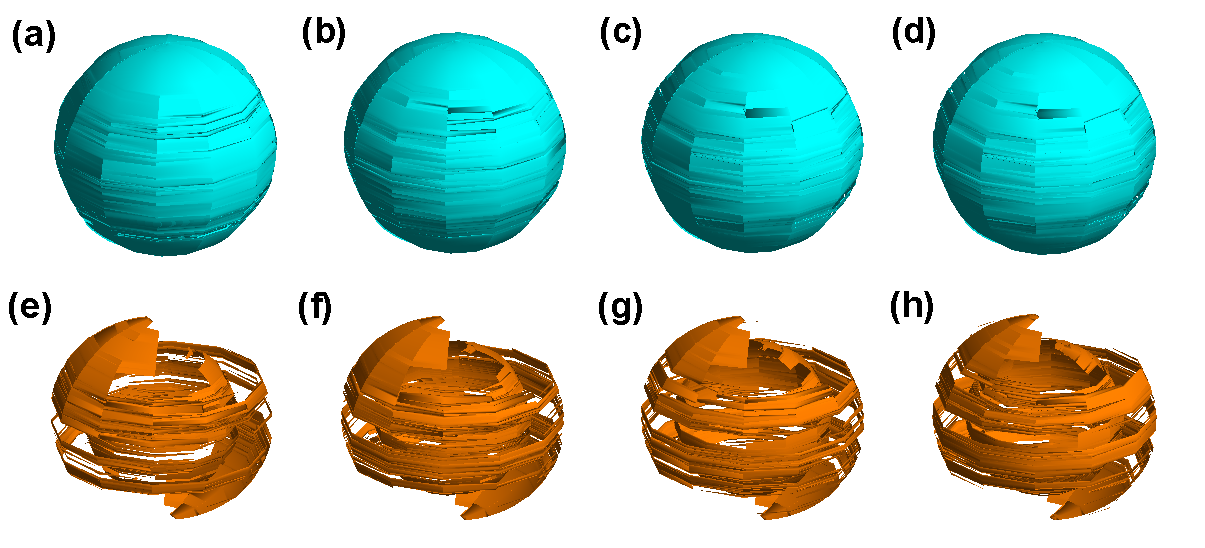
Figure 23: Instantaneous flow topology of the superfluid component in superfluid SCF with $\mbox{{Re}}=10^{3}$, $\delta=0.3$, $\Delta\Omega=0$, $\theta_{0}=3^{\circ}$, and no-slip boundary conditions on ${\bf v}_{s}$. Isosurfaces in light blue for $D_{A}=10^{-4}$ at (a) $t=20$, (b) $t=30$, (c) $t=40$, and (d) $t=50$; and in orange for $D_{A}=-10^{-4}$ at (e) $t=20$, (f) $t=30$, (g) $t=40$, and (h) $t=50$. Spectral resolution and filter parameters: $(N_{r},N_{\theta},N_{\phi})=(100,200,12)$, $(\gamma_{r},\gamma_{\theta})=(10,10)$.

Figure 24: Instantaneous flow topology of the normal fluid component in superfluid SCF with $\mbox{{Re}}=10^{4}$, $\delta=0.3$, $\Delta\Omega=0$, $\theta_{0}=3^{\circ}$, and no-slip boundary conditions on ${\bf v}_{s}$. Isosurfaces in light blue for $D_{A}=10^{-4}$ at (a) $t=20$, (b) $t=30$, (c) $t=40$, and (d) $t=50$; and in orange for $D_{A}=-10^{-4}$ at (e) $t=20$, (f) $t=30$, (g) $t=40$, and (h) $t=50$. Spectral resolution and filter parameters: $(N_{r},N_{\theta},N_{\phi})=(100,200,12)$, $(\gamma_{r},\gamma_{\theta})=(10,10)$.

Figure 25: Isosurfaces of vorticity for superfluid SCF with $\mbox{{Re}}=10^{4}$, $\delta=0.3$, $\Delta\Omega=0$, $\theta_{0}=3^{\circ}$, and no-slip boundary conditions on ${\bf v}_{s}$. Snapshots of the normal component $(\boldsymbol{\omega}_{n})_{\phi}$ are shown at times (a) $t=10$, (b) $t=20$, (c) $t=30$, (d) $t=40$, and (e) $t=50$. Snapshots of the superfluid component $(\boldsymbol{\omega}_{s})_{\phi}$ are shown at times (f) $t=10$, (g) $t=20$, (h) $t=30$, (i) $t=40$, and (j) $t=50$. Positive vorticity $(\boldsymbol{\omega}_{n,s})_{\phi}=0.1$ is shown in light blue; negative vorticity $(\boldsymbol{\omega}_{n,s})_{\phi}=-0.1$ is shown in orange. Spectral resolution and filter parameters: $(N_{r},N_{\theta},N_{\phi})=(100,200,12)$, $(\gamma_{r},\gamma_{\theta})=(10,10)$.

6.2.2 Unsteady torque

We present the evolution of the torque on the outer sphere in Figures 26 ($\mbox{{Re}}=10^{3}$) and 27 ($\mbox{{Re}}=10^{4}$). For $\mbox{{Re}}=10^{3}$, we have $N_{z}\sim 10N_{y}$, and $N_{z}\sim 40N_{x}$, as expected for small $\theta_{0}$. Moreover, $N_{z}$ tends to a constant value $N_{z}\approx 1.7\times 10^{-3}$ for the outer torque and $N_{z}\approx 1.4\times 10^{-3}$ for the inner torque at $t\geq 20$. The boundary condition on ${\bf v}_{s}$ has a negligible effect. When it is changed from no slip to perfect slip, $N_{z}$ decreases by $\mathrel{\hbox to0.0pt{\lower 4.0pt\hbox{\hskip 1.0pt$\sim$}\hss}\raise 1.0pt\hbox{$<$}}0.3$ %, and $N_{y}$ decreases by $1$ % (dashed curve in Figure 26b). For $\mbox{{Re}}=10^{4}$, the torque tends to a constant value more gradually than for $\mbox{{Re}}=10^{3}$. The differences between no slip (dashed curves) and perfect slip (solid curves) are slightly greater; $N_{x}$ and $N_{y}$ (see Figures 27a–b and 27d–e) are $\sim 2$ % larger for no slip. Again, the dominant torque component is $N_{z}$ ($>N_{y}>N_{x}$).

The differences in the torque components arise from asymmetries in the flow. In an axisymmetric flow, the greatest contribution to the torque comes from regions containing a larger number of tightly packed circulation cells. The same is true in a nonaxisymmetric flow. We calculate the torque from ${\bf N}=\int dS(\tau_{r\theta}{\bf e}_{\theta}+\tau_{r\phi}{\bf e}_{\phi})$, where $dS$ denotes the area element on the sphere and $\tau_{ij}$ are the shear stresses. We have $\tau_{r\theta}\neq 0$ and $\tau_{r\phi}\neq 0$ in a nonaxisymmetric flow, giving $N_{x}\neq 0$ and $N_{y}\neq 0$. Note that $N_{x}\neq N_{y}$ when avergared over time, since the rotation axis is in the $x$-$z$ plane.

Figure 26: Inner (left) and outer (right) torque versus time in superfluid SCF with no-slip (solid curve) and perfect-slip (dashed curve) boundary conditions on ${\bf v}_{s}$, with $\mbox{{Re}}=10^{3}$, $\delta=0.3$, $\Delta\Omega=0$, $\theta_{0}=3^{\circ}$, and GM mutual friction. From top to bottom, the plots show the (a) $x$, (b) $y$, and (c) $z$ components of the inner torque, and the (d) $x$, (e) $y$, and (f) $z$ components of the outer torque. Spectral resolution: $(N_{r},N_{\theta},N_{\phi})=(100,200,12)$. Filter parameters: $(\gamma_{r},\gamma_{\theta})=(10,10)$.

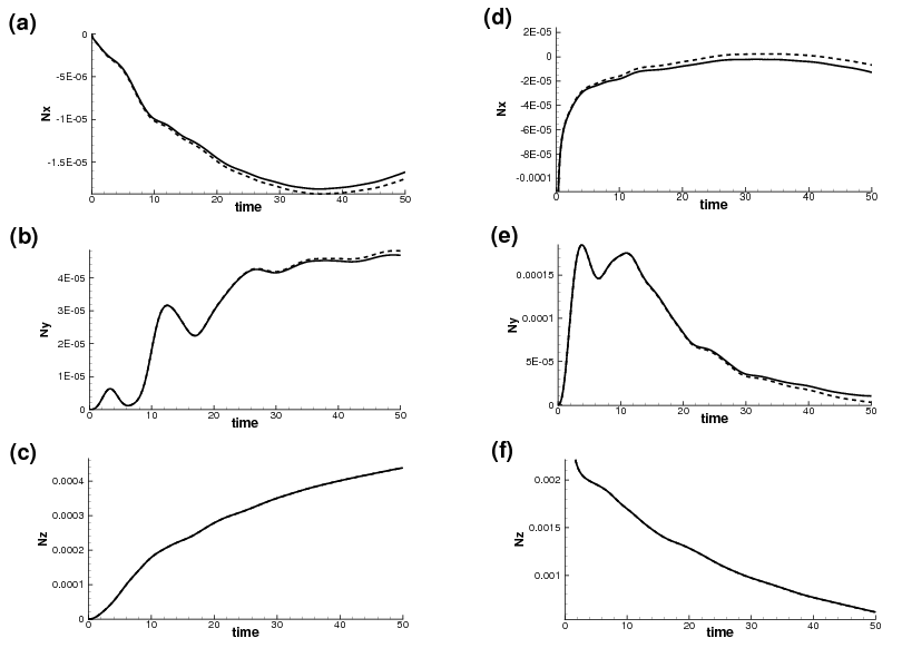
Figure 27: Inner (left) and outer (right) torque versus time in superfluid SCF with no-slip (solid curve) and perfect-slip (dashed curve) boundary conditions on ${\bf v}_{s}$, with $\mbox{{Re}}=10^{4}$, $\delta=0.3$, $\Delta\Omega=0$, $\theta_{0}=3^{\circ}$, and GM mutual friction. From top to bottom, the plots show the (a) $x$, (b) $y$, and (c) $z$ components of the inner torque, and the (d) $x$, (e) $y$, and (f) $z$ components of the outer torque. Spectral resolution: $(N_{r},N_{\theta},N_{\phi})=(100,200,12)$. Filter parameters: $(\gamma_{r},\gamma_{\theta})=(10,10)$.

6.3 Free precession

In this section, we consider a spherical rotating shell filled with superfluid, where the outer sphere precesses freely, while the inner sphere rotates uniformly. We exaggerate the biaxiality of the outer shell, taking $\Omega_{p}=1.0$ for the body-frame precessional frequency (defined in Section 3.5.4) and $\Omega^{\prime}=2.0$ for the inertial-frame precession frequency (Landau & Lifshitz, 1969; Jones & Andersson, 2001). This allows us to investigate all the time-scales comprising the precession dynamics using simulations of reasonable duration, something that would be impossible for $\Omega_{p}\ll\Omega^{\prime}$. The fixed angular momentum vector of the outer sphere points in the $z$ direction in the inertial frame of the inner sphere (which rotates with $\Omega_{1}=1.0$). An expression for the velocity of every point on the outer sphere is given in Section 3.5.4. We consider a relatively low Reynolds number, $\mbox{{Re}}=10^{3}$, with $\delta=0.3$ and no-slip boundary conditions on ${\bf v}_{s}$.

6.3.1 Topology of the flow

The topology of the flow is illustrated in Figure 28 for the normal fluid component and in Figure 29 for the superfluid component. Unlike the misaligned spheres in Section 6.2, this flow is influenced equally by strain and vorticity. The UF/C topology is slightly more prevalent (see the light blue isosurfaces in Figures 28a–d) than the SN/S/S topology in the normal fluid component. In the superfluid component, the UF/C and SN/S/S topologies are equally prevalent. The UF/C regions (in light blue in Figures 28a–d) exhibit a complicated brick-like structure (for $N_{\phi}=12$), while the SN/S/S regions are more filamentary. The superfluid component is similar to the normal fluid component but has smoother isosurfaces (see Figure 29), so it is doubly difficult to distinguish transients in the flow.

When we plot isosurfaces of vorticity, in the same manner as in Figure 25, the results are unsatisfactory. The positive and negative isosurfaces are tightly interleaved and it is hard to make out the underlying topology. However, the results improve dramatically when we subtract the vorticity of the Stokes solution from the total vorticity and project $\Delta\boldsymbol{\omega}_{n,s}$ along the instantaneous principal axis of inertia, ${\bf e}_{3}(t)$, of the outer sphere (defined in Section 3.5.4). We present isosurfaces for $\Delta\boldsymbol{\omega}_{n}\cdot{\bf e}_{3}=\pm 0.1$ in Figures 30a–d; as before, positive (negative) isosurfaces are coloured light blue (orange). Similarly, we present isosurfaces for $\Delta\boldsymbol{\omega}_{s}\cdot{\bf e}_{3}=\pm 0.1$ in Figures 30e–h. We observe that isosurfaces of $\Delta\boldsymbol{\omega}_{n}\cdot{\bf e}_{3}$ form two interlocking ribbons of opposite sign which attach ($t=20$), detach ($t=40$), and attach again ($t=50$) at two equatorial points (one of which is framed by a black circle). In contrast, isosurfaces of $\Delta\boldsymbol{\omega}_{s}\cdot{\bf e}_{3}$ exhibit a tongue-like structure in the equatorial plane (framed by a black square), which grows clockwise from $t=20$ to $t=40$ and finally develops sawteeth at $t=50$ (see Figures 30e–h). We suspect that these three-dimensional structures are not completely developed by $t=50$, i.e. we are observing transients, but computational limitations prevented us from extending the runs at the time of writing.

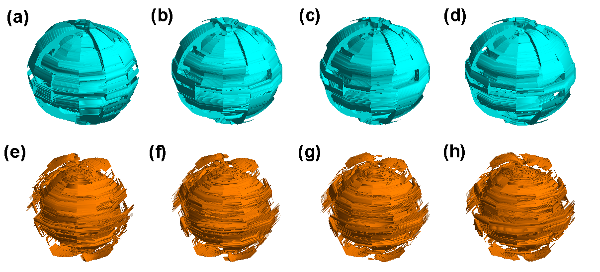
Figure 28: Instantaneous flow topology for a rotating superfluid contained within a freely precessing outer sphere and uniformly rotating inner sphere. Discriminant isosurfaces are shown for the normal fluid component, for $D_{A}=10^{-4}$ (light blue) at (a) $t=20$, (b) $t=30$, (c) $t=40$, and (d) $t=50$, and for $D_{A}=-10^{-4}$ (orange), at (e) $t=20$, (f) $t=30$, (g) $t=40$, and (h) $t=50$. The mutual friction is of GM form. Simulation parameters: $\mbox{{Re}}=10^{3}$, $\delta=0.3$, $\Omega_{1}=1.0$, $\Omega^{\prime}=2.0$, $\Omega_{p}=2.0$, $\theta_{p}=3^{\circ}$, and no-slip boundary conditions on ${\bf v}_{s}$. Spectral resolution and filter parameters: $(N_{r},N_{\theta},N_{\phi})=(100,200,12)$, $(\gamma_{r},\gamma_{\theta})=(8,8)$.

Figure 29: Instantaneous flow topology for a rotating superfluid contained within a freely precessing outer sphere and uniformly rotating inner sphere. Discriminant isosurfaces are shown for the superfluid component, for $D_{A}=10^{-4}$ (light blue), at (a) $t=20$, (b) $t=30$, (c) $t=40$, and (d) $t=50$, and for $D_{A}=-10^{-4}$ (orange) at (e) $t=20$, (f) $t=30$, (g) $t=40$, and (h) $t=50$. The mutual friction is of GM form. Simulation parameters: $\mbox{{Re}}=10^{3}$, $\delta=0.3$, $\Omega_{1}=1.0$ $\Omega^{\prime}=2.0$, $\Omega_{p}=1.0$, $\theta_{p}=3^{\circ}$, and no-slip boundary conditions on ${\bf v}_{s}$. Spectral resolution and filter parameters: $(N_{r},N_{\theta},N_{\phi})=(100,200,12)$, $(\gamma_{r},\gamma_{\theta})=(8,8)$.

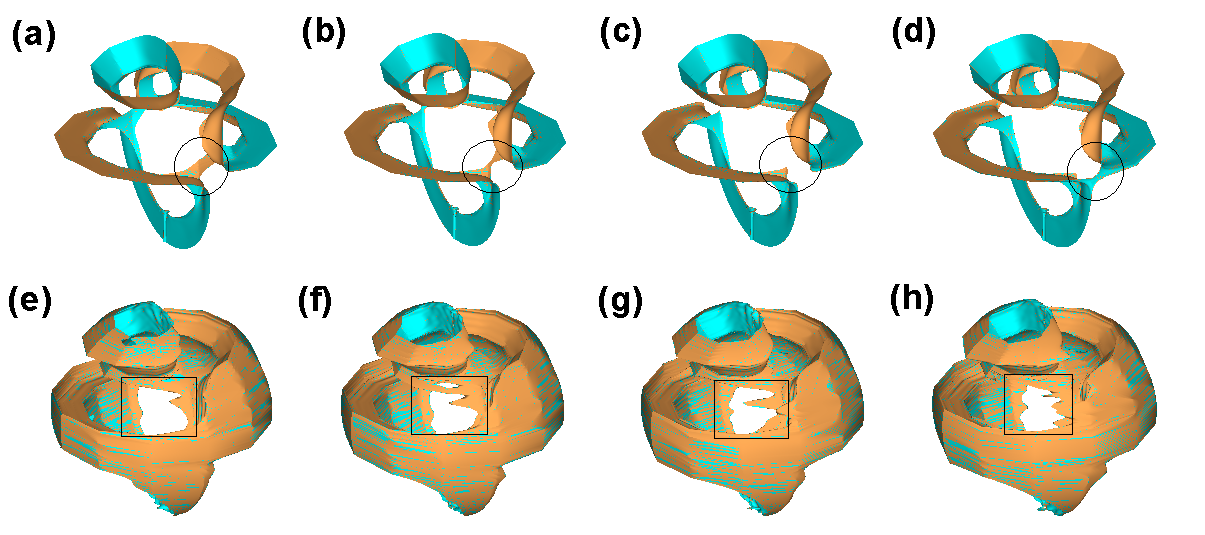
Figure 30: Isosurfaces of vorticity with the Stokes solution subtracted, projected along the instantaneous principal axis of inertia of the outer sphere. Snapshots of $\Delta\boldsymbol{\omega}_{n}\cdot{\bf e}_{3}$ are shown at times (a) $t=20$, (b) $t=30$, (c) $t=40$, and (d) $t=50$, and of $\Delta\boldsymbol{\omega}_{s}\cdot{\bf e}_{3}$ at times (e) $t=20$, (f) $t=30$, (g) $t=40$, and (h) $t=50$. Positive vorticity ($\Delta\boldsymbol{\omega}_{n,s}\cdot{\bf e}_{3}=0.1$) is shown in light blue; negative vorticity ($\Delta\boldsymbol{\omega}_{n,s}\cdot{\bf e}_{3}=-0.1$) is shown in orange. Simulation parameters: $\mbox{{Re}}=10^{3}$, $\delta=0.3$, $\Omega_{1}=1.0$, $\Omega^{\prime}=2.0$, $\Omega_{p}=1.0$, $\theta_{p}=3^{\circ}$, and no-slip boundary conditions on ${\bf v}_{s}$. Spectral resolution and filter parameters: $(N_{r},N_{\theta},N_{\phi})=(100,200,12)$, $(\gamma_{r},\gamma_{\theta})=(8,8)$.

6.3.2 Unsteady torque

In Figure 31, we plot the viscous torque exerted by the fluid on the inner (Figures 31a–c) and outer (Figures 31d–f) spheres for $\mbox{{Re}}=10^{3}$. On the inner sphere, we find $N_{z}\sim 10^{2}N_{x}\sim 10^{2}N_{y}$. On the outer sphere, we find $N_{z}\sim N_{x}\sim 10N_{y}$. The outer torque increases linearly up to $t\approx 20$, when it reaches $|N_{z}|\approx 0.03$, while the inner torque decreases to $|N_{z}|\approx 0.01$ over the same interval and oscillates persistently ($\Delta|N_{z}|\approx 10^{-3}$, period $\approx 3$). The other torque components oscillate persistently for $t\geq 2$. For example, $({\bf N}_{2})_{x}$ has constant amplitude ($\approx 4\times 10^{-2}$) and period ($\approx 3$), $({\bf N}_{1})_{x}$ has a smaller amplitude ($\approx 2\times 10^{-4}$) but the same period, $({\bf N}_{1})_{y}$ has period $\approx 3$ and amplitude ranging from $2\times 10^{-4}$ to $4\times 10^{-4}$, and $({\bf N}_{2})_{y}$ has amplitude ranging from $2\times 10^{-3}$ to $5\times 10^{-4}$.

Figure 31: Evolution of the viscous torque on the inner (left) and outer (right) spheres for a rotating superfluid contained within a freely precessing outer sphere and uniformly rotating inner sphere. From top to bottom, the plots show the (a) $x$, (b) $y$, and (c) $z$ components of the inner torque and the (d) $x$, (e) $y$, and (f) $z$ components of the outer torque. Simulation parameters: $\mbox{{Re}}=10^{3}$, $\delta=0.3$, $\Omega^{\prime}=2.0$, $\Omega_{p}=1.0$, $\Omega_{1}=1.0$, $\theta_{p}=3^{\circ}$, no-slip boundary conditions on ${\bf v}_{s}$, and GM mutual friction. Spectral resolution and filter parameters: $(N_{r},N_{\theta},N_{\phi})=(100,200,12)$, $(\gamma_{r},\gamma_{\theta})=(8,8)$.

7 Conclusion

Superfluid SCF, like its classical (Navier–Stokes) counterpart, is controlled by three global parameters: the dimensionless gap width $\delta$, the Reynolds number Re, and the rotational shear $\Delta\Omega/\Omega$. In addition, it is a function of the form (isotropic versus anisotropic) and dimensionless amplitude of the mutual friction and vortex tension forces. In this paper, we solve numerically the HVBK equations describing superfluid SCF for a range of $\delta$, Re, and $\Delta\Omega/\Omega$ and study the time-dependent behaviour of the resulting flow. The numerical solver is based upon a pseudospectral collocation method. Special attention is paid to the pole parity problem and to controlling the growth of global oscillations (due to the Gibbs phenomenon) by filtering out high spatial frequencies spectrally. The solver accurately resolves flows covering the parameter range $10\leq\mbox{{Re}}\leq 10^{5}$, $0.2\leq\delta\leq 0.9$, and $0\leq\Delta\Omega/\Omega\leq 0.3$. Grids with resolution $(N_{r},N_{\theta},N_{\phi})=(150,400,4)$ and $(100,200,12)$ are adopted for the most challenging problems we attempt in two and three dimensions respectively.

In two dimensional superfluid SCF, persistent quasiperiodic oscillations are always observed in the torque during steady differential rotation (after initial transients die away), with typical period $\sim\Omega_{1}^{-1}$ and fractional amplitude $\sim 10^{-2}$. The oscillation amplitude increases as Re increases. The viscous torques exerted by a Navier–Stokes fluid and an HVBK superfluid with GM mutual friction differ by $6$ %. However, the torque roughly triples for HV mutual friction. The meridional streamlines are more complicated for HV friction, with more small circulation cells near the outer sphere, and the amplitude of the torque oscillations is greater.

In three dimensional superfluid SCF, nonaxisymmetric vortex structures are classified according to topological invariants. The discriminant criterion is more instructive than the $\lambda_{2}$ criterion. For misaligned spheres, the flow is focal (vorticity-dominated) throughout most of its volume, except for thread-like zones where it is strain-dominated near the equator (inviscid component) and poles (viscous component). A wedge-shaped isosurface of vorticity rotates around the equator at roughly the rotation period. For a freely precessing outer sphere, the flow is equally strain- and vorticity-dominated throughout its volume. Unstable focus/contracting points are slightly more common than stable node/saddle/saddle points in the viscous component but not in the inviscid component. Isosurfaces of positive and negative vorticity form interlocking poloidal ribbons (viscous component) or toroidal tongues (inviscid component) which attach and detach at roughly the rotation period. Persistent torque oscillations are observed in all the three dimensional flows considered, with period $\sim 6\Omega_{1}^{-1}$.

A detailed knowledge of the global superfluid hydrodynamics inside a neutron star is needed to understand the origin of the timing irregularities — glitches and timing noise — observed in over $100$ radio pulsars to date (D’Alessandro et al., 1995; Shemar & Lyne, 1996; Lyne et al., 2000; Hobbs, 2002; Scott et al., 2003; Hobbs et al., 2004; Peralta et al., 2005, 2006a, 2006b; Melatos et al., 2007). Glitches are characterized by a sudden increase in the angular velocity of the pulsar, in the range $10^{-11}\mathrel{\hbox to0.0pt{\lower 4.0pt\hbox{\hskip 1.0pt$\sim$}\hss}\raise 1.0pt\hbox{$<$}}\Delta\Omega/\Omega\mathrel{\hbox to0.0pt{\lower 4.0pt\hbox{\hskip 1.0pt$\sim$}\hss}\raise 1.0pt\hbox{$<$}}10^{-4}$ (Lyne & Graham-Smith, 2006; Peralta, 2006). Pulsars also exhibit non-Gaussian fluctuations in pulse arrival times over many years, known as timing noise. The long relaxation time following a glitch, and the temperatures in a neutron star, independently imply that the interior of the star is a neutron superfluid (Lorimer & Kramer, 2004; Lyne & Graham-Smith, 2006).

Recently, it was shown that the global pattern of superfluid circulation in a neutron star exerts a dramatic influence on its rotation and may play a central role in explaining the phenomena of glitches and timing noise (Peralta et al., 2005, 2006a, 2006b). For this reason, it is important to understand more fully the axisymmetric and nonaxisymmetric dynamics of superfluid SCF. The results in this paper represent a first step along this path. One particular consequence is that, if the meridional circulation is fast enough, a vortex tangle (superfluid turbulence) is alternatively created and destroyed in the outer core of the star (and indeed any spherical container). For example, before a glitch, differential rotation in the outer core drives a nonzero, poloidal counterflow which excites the Donnelly-Glaberson instability (DGI) (Glaberson et al., 1974; Swanson et al., 1983; Tsubota et al., 2003), and the vortices evolve into an isotropic tangle of reconnecting loops. In this regime, the friction force is of GM form, coupling the normal and superfluid components loosely. Right after a glitch, the differential rotation ceases, so does the poloidal counterflow, the vortex tangle decays, a rectilinear vortex array forms, and the mutual friction changes to HV form, suddenly locking the normal and superfluid components together. In previous simulations done for neutron star parameters (Peralta et al., 2005), we make an order-of-magnitude estimate of the ratio $|{\bf F}_{\rm HV}|/{\bf F}_{\rm GM}|$ as follows. Ignoring $B^{\prime}$, we find $|{\bf F}_{\rm HV}|/{\bf F}_{\rm GM}|\sim[B\omega_{s}(v_{ns}-\nu_{s}/R_{2})]/[A^{\prime}\rho_{n}\rho_{s}v_{ns}^{3}/\kappa\rho^{2}]$. Taking $v_{ns}\sim R_{2}\Omega_{2}$, with $R_{2}\sim 10^{6}$ cm, $\Omega_{2}\sim 10^{2}$ Hz, and $A^{\prime}\sim 10^{-5}$, we get $|{\bf F}_{\rm HV}|/{\bf F}_{\rm GM}|\sim 10^{6}$. From the numerical simulations, we obtain a typical value $|{\bf F}_{\rm HV}|/{\bf F}_{\rm GM}|\sim 10^{5}$, which is similar. Nevertheless, we note that the microphysics of the GM force in superfluid turbulence has not been worked out fully yet (Jou & Mongiovì, 2004).

The results on superfluid turbulence summarised above are also relevant to laboratory experiments by Tsakadze & Tsakadze (1972, 1973, 1974, 1975, 1980), the only systematic experimental study of spherical Couette flow in superfluid helium undertaken to date. Tsakadze & Tsakadze (1972) studied the deceleration of axisymmetric vessels made of glass and plastic and filled with ⁴He (in the temperature range $1.4\,{\rm K}\leq T\leq 2.0$ K), after an impulsive acceleration. They observed “jerky” behavior, reminiscent of pulsar glitches, and developed an empirical formula for the relaxation time as a function of the initial angular velocity, the normal fluid fraction, and the radius of the vessel. The results agree qualitatively with glitch data from the Crab and Vela. These experiments lend support to the idea that the neutron superfluid inside pulsars plays an important role in the glitch phenomenon. More broadly, however, the Tsakadze experiments — and by extension, the theoretical results in this paper — are of general interest in understanding the physics of superfluid turbulence in rotating systems (Barenghi et al., 2001). The spin-up problem in helium II, and superfluids in general, is far more complicated than in a viscous fluid, because the normal fluid component interacts nonlinearly with the quantized Feynman-Onsager vortices in the superfluid component. One interesting effect is that sudden, “glitch-like”, spin-up events and other rotational irregularities are associated with patchy mutual friction: the DGI is excited in parts of the superfluid (e.g. near the walls, on the rotation axis, and at the equator) but not elsewhere (Peralta et al., 2006b). This new phenomenon will be investigated further in a forthcoming paper (Peralta et al., 2007).

Appendix A Pseudospectral collocation grids

The radial direction ($r$) is discretized using Chebyshev polynomials and a collocation scheme (Boyd, 2001). The Gauss-Lobatto collocation points in $r$ are defined as (Canuto et al., 1988)

$$x_{i}=-\cos\left[\frac{\pi(i-1)}{N_{r}-1}\right],\hskip 28.45274pt\mbox{with}\,\,\,1\leq i\leq N_{r},$$ (31)

where $N_{r}$ is the number of radial collocation points. The computational points $r_{i}$ in physical space are related to the Chebyshev grid $x_{i}$ through the mapping

$$r_{i}=x_{i}\left(\frac{R_{2}-R_{1}}{2}\right)+\left(\frac{R_{1}+R_{2}}{2}\right).$$ (32)

The angular directions $\theta$ and $\phi$ are discretized using a periodic grid over the intervals $0\leq\theta\leq\pi$ and $0\leq\phi\leq 2\pi$ respectively. In the azimuthal direction, the collocation points are defined as

$$\phi_{k}=\frac{2\pi(k-1)}{N_{\phi}},\hskip 28.45274pt\mbox{with}\,\,\,1\leq k\leq N_{\phi},$$ (33)

where $N_{\phi}$ is the number of grid points in $\phi$. In the polar direction, the collocation points are defined as

$$\theta_{j}=\frac{\pi(j-1/2)}{N_{\theta}},\hskip 28.45274pt\mbox{with}\,\,\,1\leq j\leq N_{\theta},$$ (34)

where $N_{\theta}$ is the number of grid points in $\theta$.

Appendix B Spectral expansions

A scalar field $s$ (such as pressure) is expanded as

$$s=\left\{\begin{array}[]{lll}\displaystyle\sum_{l=0}^{N_{r}-1}\sum_{j=0}^{N_{\theta}-1}\sum_{k=-N_{\phi}/2}^{N_{\phi}/2}\alpha_{ljk}T_{l}(r)\cos(j\theta)e^{ik\phi}&\,\,\mbox{for}\,\,k\,\,\mbox{even}&\\ \displaystyle\sum_{l=0}^{N_{r}-1}\sum_{j=1}^{N_{\theta}}\sum_{k=-N_{\phi}/2}^{N_{\phi}/2}\alpha_{ljk}T_{l}(r)\sin(j\theta)e^{ik\phi}&\,\,\mbox{for}\,\,k\,\,\mbox{odd}&\end{array}\right.$$ (35)

The radial component of a vector is continuous across the poles, but the tangential and azimuthal components change sign. Hence the radial, tangential, and azimuthal components of the velocity field are expanded as

$$u_{r}=\left\{\begin{array}[]{lll}\displaystyle\sum_{l=0}^{N_{r}-1}\sum_{j=0}^{N_{\theta}-1}\sum_{k=-N_{\phi}/2}^{N_{\phi}/2}\beta_{ljk}T_{l}(r)\cos(j\theta)e^{ik\phi}&\,\,\mbox{for}\,\,k\,\,\mbox{even}&\\ \displaystyle\sum_{l=0}^{N_{r}-1}\sum_{j=1}^{N_{\theta}}\sum_{k=-N_{\phi}/2}^{N_{\phi}/2}\beta_{ljk}T_{l}(r)\sin(j\theta)e^{ik\phi}&\,\,\mbox{for}\,\,k\,\,\mbox{odd}&\end{array}\right.$$ (36)

$$u_{\theta}=\left\{\begin{array}[]{lll}\displaystyle\sum_{l=0}^{N_{r}-1}\sum_{j=1}^{N_{\theta}}\sum_{k=-N_{\phi}/2}^{N_{\phi}/2}\gamma_{ljk}T_{l}(r)\sin(j\theta)e^{ik\phi}&\,\,\mbox{for}\,\,k\,\,\mbox{even}&\\ \displaystyle\sum_{l=0}^{N_{r}-1}\sum_{j=0}^{N_{\theta}-1}\sum_{k=-N_{\phi}/2}^{N_{\phi}/2}\gamma_{ljk}T_{l}(r)\cos(j\theta)e^{ik\phi}&\,\,\mbox{for}\,\,k\,\,\mbox{odd}&\end{array}\right.$$ (37)

$$u_{\phi}=\left\{\begin{array}[]{lll}\displaystyle\sum_{l=0}^{N_{r}-1}\sum_{j=1}^{N_{\theta}}\sum_{k=-N_{\phi}/2}^{N_{\phi}/2}\delta_{ljk}T_{l}(r)\sin(j\theta)e^{ik\phi}&\,\,\mbox{for}\,\,k\,\,\mbox{even}&\\ \displaystyle\sum_{l=0}^{N_{r}-1}\sum_{j=0}^{N_{\theta}-1}\sum_{k=-N_{\phi}/2}^{N_{\phi}/2}\delta_{ljk}T_{l}(r)\cos(j\theta)e^{ik\phi}&\,\,\mbox{for}\,\,k\,\,\mbox{odd}&\end{array}\right.$$ (38)

where $T_{l}$ is the $l$-th Chebyshev polynomial, $j$ and $k$ are the $\theta$ and $\phi$ wavenumbers, and $\alpha_{ljk}$, $\beta_{ljk}$, $\gamma_{ljk}$ and $\delta_{ljk}$ are real coefficients.

Appendix C Solution Algorithm

C.1 Numerical differentiation

Spatial differentiation in $r$ and $\theta$ is carried out in physical space. The first-order $r$ derivative is calculated by performing the operation

$$\frac{\partial f}{\partial r}=\displaystyle\sum_{j=1}^{N_{r}}{\cal D}_{ij}^{r}f(x_{j}),\,\,\,\,\,\,\,\,\,\,\mbox{with}\,\,\,\,\,\,1\leq i\leq N_{r},$$ (39)

in which $f(x_{j})$ is a discrete vector array, and ${\cal D}^{(r)}_{ij}$ is the differentiation operator for the variable $r$, defined below. A similar formula applies for $\partial f/\partial\theta$.

For the Gauss-Lobatto distribution of radial points defined in Section 3.1, the radial derivative operator is defined as

$${\cal D}_{ij}^{r}=\left\{\begin{array}[]{ll}\displaystyle\displaystyle\frac{(-1)^{i+j}}{\displaystyle 2\sin\left[\frac{\pi}{2(N_{r}-1)(i+j-2)}\right]\displaystyle\sin\left[\frac{\pi(i-j)}{2(N_{r}-1)}\right]}&\,\,\,\,\,\mbox{for}\,\,i\neq j\\ \\ \displaystyle\frac{\displaystyle\cos[\pi j/(N_{r}-1)]}{\displaystyle 2\sin^{2}[\pi j/(N_{r}-1)]}&\,\,\,\,\,\mbox{for}\,\,i<=j<N_{r}\\ \\ \displaystyle-\frac{2(N_{r}-1)^{2}+1}{6}&\,\,\,\,\,\mbox{for}\,\,i=j=1\\ \\ \displaystyle\frac{2(N_{r}-1)^{2}+1}{6}&\,\,\,\,\,\mbox{for}\,\,i=j=N_{r}.\end{array}\right.$$ (40)

The top-half entries of the matrix ${\cal D}_{ij}^{r}$ ($1\leq i,j\leq N_{r}/2$) are more accurately represented than the lower-half ones, for a given machine precision $\epsilon$ (Don & Solomonoff, 1995). A significant improvement in accuracy is obtained by using the property ${\cal D}_{ij}^{r}=-{\cal D}_{{N_{r}-i},{N_{r}-j}}^{r}$ [for $(N_{r}/2)+1\leq i\leq N_{r}$], and calculating only the more accurate top-half part of (40). This reduces the overall round-off error from ${\cal O}(N_{r}^{3}\epsilon)$ to ${\cal O}(N_{r}^{2}\epsilon)$ (Don & Solomonoff, 1995). Radial derivatives of order $n$ are computed by applying (40) $n$ times.

For a periodic grid with $2N_{\theta}$ points, the first-order $\theta$ differentiation operator can be expressed as (Canuto et al., 1988)

$${\cal F}_{ij}^{\theta}=\left\{\begin{array}[]{ll}\displaystyle\frac{1}{2}\displaystyle(-1)^{i-j}\cot\displaystyle\frac{\pi(i-j)}{2N_{\theta}}&\hskip 28.45274pt\,\,\,\,\mbox{for}\,\,i\neq j\\ \\ 0&\hskip 28.45274pt\,\,\,\,\mbox{for}\,\,i=j,\end{array}\right.$$ (41)

and the second-order differentiation operator as

$${\cal F}_{ij}^{\theta\theta}=\left\{\begin{array}[]{ll}\displaystyle\frac{1}{2}\displaystyle(-1)^{i-j+1}\sin^{2}\displaystyle\frac{\pi(i-j)}{2N_{\theta}},&\,\,\,\,\,\,\mbox{for}\,\,i\neq j\\ \\ \displaystyle-\frac{2+N_{\theta}^{2}}{12},&\,\,\,\,\,\,\mbox{for}\,\,i=j.\end{array}\right.$$ (42)

The form of ${\cal D}_{ij}^{\theta}$ depends on the parity of the function $f(x_{j})$ on which it acts, as explained in Section B. First-order cosine ($\cal C$) and sine ($\cal S$) operators can be constructed from (41) as

$${\cal C}_{ij}^{\theta}={\cal F}_{ij}^{\theta}+{\cal F}_{i,2N_{\theta}+1-j}^{\theta}\hskip 28.45274pt\,\,\,\,\,\,\,\,\,\,\,\mbox{for}\,\,\,\,1\leq i,j\leq N_{\theta}$$ (43)

$${\cal S}_{ij}^{\theta}={\cal F}_{ij}^{\theta}-{\cal F}_{i,2N_{\theta}+1-j}^{\theta}\hskip 28.45274pt\,\,\,\,\,\,\,\,\,\,\,\mbox{for}\,\,\,\,1\leq i,j\leq N_{\theta},$$ (44)

and second-order cosine and sine operators can be defined as

$${\cal C}_{ij}^{\theta\theta}={\cal F}_{ij}^{\theta\theta}+{\cal F}_{i,2N_{\theta}+1-j}^{\theta\theta}\hskip 28.45274pt\,\,\,\,\,\,\,\,\,\,\,\mbox{for}\,\,\,\,1\leq i,j\leq N_{\theta}$$ (45)

$${\cal S}_{ij}^{\theta\theta}={\cal F}_{ij}^{\theta\theta}-{\cal F}_{i,2N_{\theta}+1-j}^{\theta\theta}\hskip 28.45274pt\,\,\,\,\,\,\,\,\,\,\,\mbox{for}\,\,\,\,1\leq i,j\leq N_{\theta}.$$ (46)

The operators (43)–(46) are applied in spectral space using a fast Fourier transform (FFT). Since the expansions (35)–(38) are different for even or odd $k$, the $\theta$ differentiation is performed separately for even and odd $k$. For even $k$, a $\cal C$ operator is applied; for odd $k$, an $\cal S$ operator is applied . The differentiation operator reverses the parity when applied an odd number of times and leaves the parity unchanged when applied an even number of times, which needs to be taken into account when computing higher order derivatives.

For the $\phi$ derivatives, the periodicity of the grid makes it easier to perform the differentiation in spectral space. Differentiation in $\phi$ reduces to multiplying each Fourier coefficient ${\rm FFT}_{\phi}[f(x_{k})]=\widehat{f}(x_{k})$ by $i=\sqrt{-1}$ times the corresponding wavenumber $k$, viz.

$${\cal D}^{\phi}\widehat{f}(x_{j})=ik\widehat{f}(x_{j})\hskip 56.9055pt\,\,\mbox{for}\,\,1\leq j\leq N_{r,\theta}.$$ (47)

The function $\widehat{f}(x_{j})$ is transformed back to physical space using an inverse FFT. In order to compute $\phi$ derivatives of order $n$, the operation (47) is performed $n$ times.

C.2 Temporal discretization

The most common and efficient method to solve the Navier–Stokes equation in terms of the primitive variables (i.e., the velocity and pressure fields) is the fractional step approach (Chorin, 1968; Brown et al., 2001). This method proceeds in two time steps, decoupling the calculation of the velocity and pressure fields. In the first step, an intermediate velocity field ${\bf v}_{n,s}^{\star}$ is computed from the velocity field at the $n$-th time level, ${\bf v}_{n,s}^{n}$, using the momentum equations (1) and (2) and ignoring the pressure and the incompressibility constraint (3). In the second step, the pressure is calculated by solving a Poisson equation involving the intermediate velocity field to obtain the final, divergence-free velocity field at the $n+1$-th time level, ${\bf v}_{n,s}^{n+1}$. The second step can be seen as a projection of ${\bf v}_{n,s}$ onto a space of divergence-free vectors.

Stable evolution is achieved by treating all the viscous terms implicitly, to avoid the stringent upper bound on $\Delta t$ imposed by the CFL condition (Voigt et al., 1984). Nonlinear terms, on the other hand, are treated explicitly (Orszag, 1971a). Upon discretizing equations (1) and (2) in time using an explicit third-order Adams-Bashforth (AB3) method for the nonlinear terms and an implicit second-order Crank-Nicolson (CN2) for the viscous terms (Boyd, 2001), and advancing the solution from the time level $n$ to the time level $\star$, we obtain

$$\frac{{\bf v}_{n}^{\star}-{\bf v}_{n}^{n}}{\Delta t} = -\frac{1}{12}\left\{23\left[{\bf v}_{n}\cdot\nabla{\bf v}_{n}+\frac{\rho_{s}\nabla\omega_{s}}{\rho{\it Re_{s}}}-\frac{\rho_{s}{\bf F}}{\rho}-{D}_{\alpha}\right]^{n}-16\left[{\bf v}_{n}\cdot\nabla{\bf v}_{n}+\frac{\rho_{s}\nabla\omega_{s}}{\rho{\it Re_{s}}}\right.\right.$$ (48)

$$\left.\left.-\frac{\rho_{s}{\bf F}}{\rho}-{D}_{\alpha}\right]^{n-1}+5\left[{\bf v}_{n}\cdot\nabla{\bf v}_{n}+\frac{\rho_{s}\nabla\omega_{s}}{\rho{\it Re_{s}}}-\frac{\rho_{s}{\bf F}}{\rho}-\frac{{D}_{\alpha}}{{\it Re_{s}}}{\bf e}_{\alpha}\right]^{n-2}\right\}$$

$$+\frac{{\bf e}_{\alpha}}{2\mbox{{Re}}}\left[\frac{1}{r^{2}\sin^{2}\theta}\frac{\partial^{2}v_{n\alpha}^{\star}}{\partial\phi^{2}}+\frac{1}{r^{2}\sin^{2}\theta}\frac{\partial^{2}v_{n\alpha}^{n}}{\partial\phi^{2}}+\frac{1}{r^{2}}\frac{\partial}{\partial r}\left(r^{2}\frac{\partial v_{n\alpha}^{\star}}{\partial r}\right)\right.$$

$$\left.+\frac{1}{r^{2}}\frac{\partial}{\partial r}\left(r^{2}\frac{\partial v_{n\alpha}^{n}}{\partial r}\right)\right],$$

$$\frac{{\bf v}_{s}^{\star}-{\bf v}_{s}^{n}}{\Delta t} = \frac{1}{12}\left\{23\left[{\bf v}_{s}\cdot\nabla{\bf v}_{s}++\frac{\rho_{s}\nabla\omega_{s}}{\rho{\it Re_{s}}}+\frac{\rho_{n}{\bf F}}{\rho}+\frac{{\bf T}}{{\it Re_{s}}}\right]^{n}-16\left[{\bf v}_{s}\cdot\nabla{\bf v}_{s}+\frac{\rho_{s}\nabla\omega_{s}}{\rho{\it Re_{s}}}\right.\right.$$ (49)

$$\left.+\frac{\rho_{n}{\bf F}}{\rho}+\frac{{\bf T}}{{\it Re_{s}}}\right]^{n-1}\left.+5\left[{\bf v}_{s}\cdot\nabla{\bf v}_{s}+\frac{\rho_{s}\nabla\omega_{s}}{\rho{\it Re_{s}}}+\frac{\rho_{n}{\bf F}}{\rho}+\frac{{\bf T}}{{\it Re_{s}}}\right]^{n-2}\right\},$$

where ${\bf e}_{\alpha}=({\bf e}_{r},{\bf e}_{\theta},{\bf e}_{\phi})$ is the triad of spherical polar unit vectors. The term ${D}_{\alpha}$ is defined as

$${D}_{r} = \frac{1}{r^{2}\sin\theta}\frac{\partial}{\partial\theta}\left(\sin\theta\frac{\partial v_{nr}}{\partial\theta}\right)-\frac{2v_{nr}}{r^{2}}-\frac{2}{r^{2}}\frac{\partial v_{n\theta}}{\partial\theta}-\frac{2v_{n\theta}\cot\theta}{r^{2}}-\frac{2}{r^{2}\sin\theta}\frac{\partial v_{n\phi}}{\partial\phi},$$ (50)

$${D}_{\theta} = \frac{1}{r^{2}\sin\theta}\frac{\partial}{\partial\theta}\left(\sin\theta\frac{\partial v_{n\theta}}{\partial\theta}\right)+\frac{2}{r^{2}}\frac{\partial v_{nr}}{\partial\theta}-\frac{v_{n\theta}}{r^{2}\sin^{2}\theta}-\frac{2\cos\theta}{r^{2}\sin^{2}\theta}\frac{\partial v_{n\phi}}{\partial\phi},$$ (51)

$${D}_{\phi} = \frac{1}{r^{2}\sin\theta}\frac{\partial}{\partial\theta}\left(\sin\theta\frac{\partial v_{n\phi}}{\partial\theta}\right)-\frac{v_{n\phi}}{r^{2}\sin^{2}\theta}+\frac{2}{r^{2}\sin^{2}\theta}\frac{\partial v_{nr}}{\partial\phi}+\frac{2\cos\theta}{r^{2}\sin^{2}\theta}\frac{\partial v_{n\theta}}{\partial\phi}.$$ (52)

Note that the Laplacian operator $\nabla^{2}{\bf v}$ splits into two parts: $\theta$ derivatives are computed explicitly with an AB3 scheme, while $r$ and $\phi$ derivatives are computed implicitly with a CN2 scheme. This procedure avoids numerical instabilities (Bagchi, 2002) and allows us to rewrite equation (48) at the time level $\star$ as a Helmholtz equation for ${\bf v}_{n}^{\star}$ (see Section C.3).

The previous advection-diffusion step is followed by a pressure correction step based on

$$\frac{{\bf v}_{n,s}^{n+1}-{\bf v}_{n,s}^{\star}}{\Delta t}=-\nabla p_{n,s}^{n+1}.$$ (53)

By taking the divergence of this equation, and imposing the continuity constraint $\nabla\cdot{\bf v}_{n,s}^{n+1}=0$, we obtain a Poisson equation for the pressure:

$$\frac{\nabla\cdot{\bf v}_{n,s}^{\star}}{\Delta t}=\nabla^{2}p_{n,s}^{n+1}.$$ (54)

This equation is solved implicitly for $p_{n,s}^{n+1}$ at every time step, in order to get divergence-free normal and superfluid velocity fields accurate to second order in time.

A boundary condition is needed to solve equation (54). Since physical boundary conditions do not apply to ${\bf v}_{n,s}^{\star}$ and $p_{n,s}^{n+1}$, a number of empirical choices have been proposed (Kim & Moin, 1985; Bell et al., 1989). Unfortunately, all the choices create a spurious numerical boundary layer at the edge of the computational domain. The simplest and most common choice for the pressure is a homogeneous boundary condition $(\partial p_{nr,sr}^{n+1}/\partial r)|_{r=R_{1},R_{2}}=0$ (Orszag et al., 1986). The radial component of the velocity field satisfies no penetration, viz. ${\bf e}_{r}\cdot{\bf v}_{n,s}^{\star}={\bf e}_{r}\cdot{\bf v}_{n,s}^{n+1}=0$. A boundary condition for the tangential components can be obtained by rearranging equation (53) to read ${\bf v}_{n,s}^{\star}|_{r=R_{1},R_{2}}=({\bf v}_{n,s}^{n+1}+\Delta t\nabla p_{n,s}^{n+1})|_{\partial\Gamma}$. However, $\nabla p_{n,s}^{n+1}$ is unknown at this stage of the calculation: we wish to solve for it in order to pressure-correct the fields. Streett & Hussaini (1991) argue that, since the time-stepping scheme is second-order accurate in time, a second-order accurate (or better) estimate for the velocity fields is sufficient to preserve global second-order accuracy. Expanding $\nabla p_{n,s}^{n+1}$ in a Taylor series about $t=t^{n}$ and approximating $\partial p_{n,s}^{n}/\partial t$ with a first-order backward difference formula, we obtain $\nabla p_{n,s}^{n+1}=2\nabla p_{n,s}^{n}-\nabla p_{n,s}^{n-1}+{\cal O}(\Delta t^{2})$ and the boundary condition for the $\theta$ and $\phi$ components of the $\star$ velocity fields then becomes

$$\mbox{\boldmath$\tau$}\cdot{\bf v}_{n,s}^{\star}=\mbox{\boldmath$\tau$}\cdot\left[{\bf v}_{n,s}^{n+1}+\Delta t(2\nabla p^{n}-\nabla p^{n+1})\right]+{\cal O}(\Delta t^{3}),$$ (55)

with $\mbox{\boldmath$\tau$}={\bf e}_{\theta}$ or ${\bf e}_{\phi}$. This gives a small slip velocity at the boundary, at the time level $n+1$, of order ${\cal O}(\Delta t^{3})$. The particular choices for ${\bf v}^{n+1}_{n,s}$ are described in more detail below.

Once $p^{n+1}$ has been calculated, the updated divergence-free velocity fields ${\bf v}_{n,s}^{n+1}$ are calculated from (53). Note that, since there is no diffusive term in equation (2), the explicit AB3 method is used to advance ${\bf v}_{s}$ from the time level $n$ to the time level $\star$.

C.3 Advancing the solution in time

Starting from an initial choice of ${\bf v}_{n}$ and ${\bf v}_{s}$ that satisfies the continuity equations (3), the time-stepping procedure consists of an advection step (or, more precisely, an advection-diffusion step for the normal fluid), in which the linear terms are handled implicitly (Crank-Nicolson) and the nonlinear terms explicitly (Adams-Bashforth), followed by a pressure-correction step. Given the solution at the $n$-th time level, and appropriate boundary conditions, the algorithm proceeds as follows.

1. We calculate the Fourier and Chebyshev grids, the differentiation matrices, the matrix operations that only depend on the spatial grid needed by the Helmholtz and Poisson solvers (see below), any exponential filters to be applied to ${\bf v}_{n}$ and ${\bf v}_{s}$, and the pole filter and anti-aliasing filter matrices (see Section 3.4).

2. We calculate the nonlinear and linear parts of (48) and (49). The time-stepping loop starts. The AB3 method initializes ${\bf v}_{n,s}^{1}$ and ${\bf v}_{n,s}^{2}$ using a lower-order, Euler method.

3. We perform the advection-diffusion step. All the velocity and pressure variables are Fourier expanded in $\phi$. A Helmholtz equation (equation 56 below) is solved in order to get the intermediate ${\bf v}_{n}^{\star}$ at the time level $\star$. The AB3 algorithm is used to step forward ${\bf v}_{s}$ explicitly to the time level $\star$. The boundary conditions are applied.

4. We apply filters to the expansion coefficients and a convective filter, as described in Section 3.4. We then pressure-correct ${\bf v}_{n}^{\star}$ and ${\bf v}_{s}^{\star}$ in order to get ${\bf v}_{n}^{n+1}$ and ${\bf v}_{s}^{n+1}$, satisfying the continuity equation (3). Poisson’s equation (53) is solved for ${\bf v}_{n}^{\star}$ and ${\bf v}_{s}^{\star}$ and the solution is advanced to the time level $n+1$ using (53).

5. We take the inverse Fourier transform of the velocity and pressure fields and write out their values on the coordinate grid as a restart file (if desired).

We now describe in detail steps (c) and (d). The $r$, $\theta$ and $\phi$ components of the vector Laplacian $\nabla^{2}{\bf v}$ are coupled and a completely implicit treatment of the diffusive terms is cumbersome. To get around this issue, in step (d), the linear diffusive terms in equation (1) are treated semi-implicitly: only the linear terms in the Laplacian are included in the implicit temporal discretization (using the CN algorithm) (Bagchi, 2002), while the nonlinear terms in (1) are treated in an explicit way (using an AB3 algorithm). Since $r\Delta\theta>\Delta r$, the $\theta$ components of the Laplacian can be treated explicitly, without affecting the stability of the time-stepping algorithm (see Section C.2). Moving the nonlinear terms and $\theta$ derivatives of the Laplacian to the right-hand side of equation (48), and the time derivatives to the left-hand side, and Fourier transforming all the variables, we arrive at a Helmholtz equation for the normal velocity field ${\bf v}_{n}=(v_{nr},v_{n\theta},v_{n\phi})$ at the time step $\star$ which, for the radial component, takes the form

$$\sin^{2}\theta\frac{\partial}{\partial r}\left(r^{2}\frac{\partial\widehat{v}_{nr}^{\star}}{\partial r}\right)-\left(\frac{r^{2}\sin^{2}\theta\mbox{{Re}}}{\Delta t}+\frac{k_{\phi}}{2}\right)\widehat{v}_{nr}^{\star}=\widehat{\left(RHS\right)}^{n}_{r},$$ (56)

where all Fourier-transformed quantities are indicated by a ‘$\widehat{\hskip 7.11317pt}$’. Similar equations can be written for $\widehat{v}_{n\theta}^{\star}$ and $\widehat{v}_{n\phi}^{\star}$. The right-hand side $\widehat{\left(RHS\right)}^{n}_{r}$ contains all the non-linear terms and $\theta$ derivatives of the Laplacian evaluated at the time step $n$. This equation is solved in spectral space for each wave number $k_{\phi}$, as described below.

The absence of a viscous term in equation (2) allows us to use an explicit method for the evolution in time, as indicated in equation (49). For ${\bf v}_{s}=(v_{sr},v_{s\theta},v_{s\phi})$, the solution advances in time from $n$ to $\star$ according to an AB3 scheme,

$$\widehat{v}_{si}^{\star}=\widehat{v}_{si}^{\,n}-\Delta t\left[\frac{23}{12}\widehat{\left(NLS\right)}_{i}^{n}-\frac{4}{3}\widehat{\left(NLS\right)}_{i}^{n-1}+\frac{5}{12}\widehat{\left(NLS\right)}_{i}^{n-2}\right],$$ (57)

where $\widehat{\left(NLS\right)}_{i}$ contains all the nonlinear terms in (2).

The velocity fields obtained from equations (56) and (57) are not divergence-free, and therefore do not satisty the continuity equation. A correction must be made by solving the Poisson equation (54) for the pressure, which can be written as

$$\frac{\partial}{\partial r}\left(r^{2}\frac{\partial\widehat{p}_{n,s}^{\,n+1}}{\partial r}\right)+\frac{1}{\sin\theta}\frac{\partial}{\partial\theta}\left(\sin\theta\frac{\partial\widehat{p}_{n,s}^{\,n+1}}{\partial\theta}\right)-\frac{k_{\phi}\widehat{p}_{n,s}^{\,n+1}}{\sin^{2}\theta}=r^{2}\frac{\widehat{\nabla\cdot{\bf v}_{n,s}^{\star}}}{\Delta t}.$$ (58)

The corrected velocity fields ${\bf v}_{n}^{n+1}$ and ${\bf v}_{s}^{n+1}$ are then calculated using (53), which gives

$$\widehat{{\bf v}}_{n,s}^{n+1}=\widehat{{\bf v}}_{n,s}^{\star}-\nabla\widehat{p}_{n,s}^{n+1}\Delta t.$$ (59)

Equations (56) and (58) are solved using a matrix diagonalization method (Canuto et al., 1988; Trefethen, 2001). The Helmholtz and Poisson equations can be written in matrix form, viz.

$$\left[A\right]\left[\widehat{v}\right]+\left[\widehat{v}\right][B]^{T}-\alpha[\widehat{v}]=\widehat{\left[RHS\right]},$$ (60)

where $\left[\widehat{v}\right]$ is a $N_{r}\times N_{\theta}$ array containing the velocity or pressure fields, and $\left[A\right]$ is a $N_{r}\times N_{r}$ matrix that represents the discrete operators on the left-hand sides of (56) and (58). The matrix $\left[B\right]^{T}$ is the transpose of $\left[B\right]$, a $N_{\theta}\times N_{\theta}$ matrix which is zero for the Poisson equation (58) and contains the second and third terms in the Helmholtz equation (56). Finally, we have $\alpha=2\mbox{{Re}}/\Delta t$ for (56) and $\alpha=0$ for (58).

In order to solve equation (60) by matrix diagonalization (Canuto et al., 1988), we decompose $\left[A\right]$ and $\left[B\right]$ in eigenvectors and eigenvalues for the operators $\nabla^{2}_{r}$ and $\nabla^{2}_{\theta}$ as

$$\left[A\right]=\left[M\right]\left[\lambda_{r}\right]\left[M\right]^{-1},\quad\quad\left[B\right]=\left[N\right]\left[\lambda_{\theta}\right]\left[N\right]^{-1},$$ (61)

where $\left[M\right]$ and $\left[N\right]$ are matrices formed from the eigenvectors of $\left[\nabla^{2}_{r}\right]$ and $\left[\nabla^{2}_{\theta}\right]$, and $\left[\lambda_{r}\right]$ and $\left[\lambda_{\theta}\right]$ are diagonal matrices formed from the eigenvalues of $\left[\nabla^{2}_{r}\right]$ and $\left[\nabla^{2}_{\theta}\right]$, respectively. Substituting equation (61) in equation (60) leads to

$$\left[\lambda_{r}\right]\left[u\right]+\left[u\right]\left[\lambda_{\theta}\right]-\alpha\left[u\right]=\left[s\right],$$ (62)

with $\left[u\right]=\left[M\right]^{-1}\left[\widehat{v}\right]\left[N\right]$ and $\left[s\right]=\left[M\right]^{-1}\widehat{\left[RHS\right]}\left[N\right]$. Since $\left[\lambda_{r}\right]$ and $\left[\lambda_{\theta}\right]$ are diagonal matrices, this expression can be simplified to $[u]=[\lambda_{r}+\lambda_{\theta}-\alpha]^{-1}[s]$ and written explicitly as

$$\left[u\right]_{ij}=\frac{\left[s\right]_{ij}}{\left[\lambda_{r}\right]_{ii}+\left[\lambda_{\theta}\right]_{jj}-\alpha},\,\,\hskip 85.35826pt\mbox{for}\,\,1\leq i,j\leq N_{r,\theta}.$$ (63)

Finally, $\left[\widehat{v}\right]$ can be obtained from (63) using $\left[\widehat{v}\right]=[M][u][N]^{-1}$.

To impose boundary conditions in the $r$ and $\theta$ directions, the last and first rows of the operator matrices $\left[A\right]$ and $\left[B\right]$ must be modified to include the known boundary values on the right-hand side of the equation (Trefethen, 2001). Dirichlet boundary conditions are applied to the Helmholtz equation for ${\bf v}_{n}$ (see Section 3.5.2). Neumann boundary conditions are applied to the Poisson equation for $p_{n,s}$ (see Section C.2).

References

- Andersson & Comer (2006) Andersson, N. & Comer, G. L. 2006 A flux-conservative formalism for convective and dissipative multi-fluid systems, with application to Newtonian superfluid neutron stars. Classical Quant. Grav. 23, 5505–5529.
- Andronikashvili & Mamaladze (1966) Andronikashvili, E. L. & Mamaladze, Y. G. 1966 Quantization of Macroscopic Motions and Hydrodynamics of Rotating Helium II. Rev. Mod. Phys. 38, 567–625.
- Bagchi (2002) Bagchi, P. 2002 Particle dynamics in inhomegeneous flow at moderate to high Reynolds number. PhD thesis, University of Illinois at Urbana-Champaign.
- Bagchi & Balachandar (2002) Bagchi, P. & Balachandar, S. 2002 Steady planar straining flow past a rigid sphere at moderate Reynolds number. J. Fluid. Mech. 466, 365–407.
- Barenghi (1992) Barenghi, C. F. 1992 Vortices and the Couette flow of helium II. Phys. Rev. B 45, 2290–2293.
- Barenghi (1995) Barenghi, C. F. 1995 Superfluid Rayleigh criterion. Phys. Rev. B 52, 3596–3600.
- Barenghi et al. (1983) Barenghi, C. F., Donnelly, R. J. & Vinen, W. F. 1983 Friction on Quantized Vortices in Helium II. A Review. J. Low Temp. Phys. 52, 189–246.
- Barenghi et al. (2001) Barenghi, C. F., Donnelly, R. J. & Vinen, W. F. 2001 Quantized Vortex Dynamics and Superfluid Turbulence. LNP Vol. 571: Quantized Vortex Dynamics and Superfluid Turbulence 571.
- Barenghi & Jones (1988) Barenghi, C. F. & Jones, C. A. 1988 The stability of the Couette flow of Helium II. J. Fluid Mech. 197, 551.
- Bekarevich & Khalatnikov (1961) Bekarevich, I. L. & Khalatnikov, I. M. 1961 A phenomenological derivation of the equations of vortex motion in He II. Sov. Phys. JETP 13, 643–646.
- Bell et al. (1989) Bell, J. B., Colella, P. & Glaz, H. M. 1989 A second-order projection method for the incompressible Navier-Stokes equations. J. Comp. Phys. 85, 257–283.
- Belyaev et al. (1978) Belyaev, Yu N, Monakhov, A. A. & Yavorskaya, I. M. 1978 Stability of spherical Couette flow in thick layers when the inner sphere revolves. Fluid Dyn. 2, 162–168.
- Bonnet & Alziary de Roquefort (1976) Bonnet, J. P. & Alziary de Roquefort, T. 1976 Ecoulement entre deux sphéres concentriques en rotation rotating spheres. J. Méc. 15, 373–397.
- Boyd (2001) Boyd, J. P. 2001 Chebyshev and Fourier Spectral Methods. Dover Publications.
- Brown et al. (2001) Brown, D. L., Cortez, R. & Minion, M. L. 2001 Accurate projection methods for the incompressible Navier-Stokes equations. J. Comput. Phys. 168, 464–499.
- Bühler (1990) Bühler, K. 1990 Symmetric and asymmetric Taylor vortex flow in spherical gaps. Acta Mech. 81, 3–38.
- Canuto et al. (1988) Canuto, C., Hussaini, M., Quarteroni, A. & Zang, T. 1988 Spectral Methods in Fluid Dynamics. Springer-Verlag.
- Chong et al. (1990) Chong, M. S., Perry, A. E. & Cantwell, B. J. 1990 A general classification of three-dimensional flow fields. Phys. Fluids 2, 765–777.
- Chorin (1968) Chorin, A. J. 1968 Numerical solution of the Navier-Stokes equations. Math. Comp. 22, 745–762.
- D’Alessandro et al. (1995) D’Alessandro, F., McCulloch, P. M., Hamilton, P. A. & Deshpande, A. A. 1995 The timing noise of 45 southern pulsars. Mon. Not. R. Astron. Soc. 277, 1033–1046.