Signal propagation through dense granular systems

Abstract

The manner in which signals propagate through dense granular systems in both space and time is not well understood. In order to learn more about this process, we carry out discrete element simulations of the system response to excitations where we control the driving frequency and wavelength independently. Fourier analysis shows that properties of the signal depend strongly on the spatial and temporal scales introduced by the perturbation. The features of the response provide a test-bed for any continuum theory attempting to predict signal properties. We illustrate this connection between micro-scale physics and macro-scale behavior by comparing the system response to a simple elastic model with damping.

The issue of stress and energy transport through dense granular matter (DGM) is of significant importance to a number of applications ranging from detection of land mines to oil exploration. Due to the importance of this problem, a significant amount of research has been carried out in order to understand the basic physical mechanisms involved. The major focus of recent work on this issue has been on how the application of static forces changes the force structure within a material. One approach involves considering typically small size granular samples exposed to time-independent, often point-like perturbations. A substantial range of models has been proposed, including diffusive Coppersmith et al. (1996), wave-like Bouchaud et al. (1994); Otto et al. (2003); Blumenfeld (2004) or elastic response Goldenberg and Goldhirsch (2005). More traditional continuum models Nedderman (1992); Goddard (1990)) commonly assume an elastic or elasto-plastic response. These various models are fundamentally at odds with each other, since the basic (possibly continuum limit) equations for these different descriptions are of parabolic, hyperbolic, or elliptic nature with respect to their spatial variables. Some progress in connecting discrete and continuum descriptions has been reached by realizing that the system’s response may change depending on the scale or the state of the system: one can see wave-like response on short (meso) scales, but elastic response on longer ones Goldenberg and Goldhirsch (2005). For dense systems, theory and experiment Goldenberg and Goldhirsch (2005); Geng et al. (2003) suggest that an elastic description is best, but near jamming threshold, a hyperbolic description may apply Blumenfeld (2004).

Understanding signal (such as a compression wave) propagation through a granular system builds on the approaches used for studies of the static force response but adds the additional feature of time-dependence. Within continuum theory, the issue of ‘sound’ propagation is often considered via an effective medium approach Goddard (1990); Sheng (1995). A typical model in this class explores the response to a spatially independent perturbation which is large compared to a particle size, such as the response to a moving piston. Other work has used experiments and simulations to explore the pressure dependence of the sounds speed, and the role of microsctructure including force chains on signal propagation Makse et al. (1999); Jia (2004); Somfai et al. (2005); Hostler and Brennen (2005). Very different issues arise for 1D particle chains, which are characterized by nonlinear high-order wave-like continuum models Nesterenko (2001). An extension of these results to higher dimensions and realistic granular media remains to be carried out.

This letter concentrates on the response of DGM to space-time dependent perturbations, with the goal of gaining further insight into the mechanisms involved in stress and energy transport. To the best of our knowledge, this approach has not been considered so far. We concentrate on the regime where the imposed frequencies are low, and the wavelengths are large compared to the particle size. We then compare the information extracted from discrete element (DEM) simulations to expectations based on a simple continuum picture, that includes elastic and diffusive behavior.

We choose a relatively simple granular geometry in two spatial dimensions with the granular particles constrained between two rough walls (up-down) with periodic boundary conditions (left-right). The walls’ position prescribes the volume fraction, $\nu=0.9$. The particles are polydisperse disks, with the radii varying randomly in the range of $\pm 5\%$ about the mean. For simplicity, we put gravity to zero. The particle-particle and particle-wall interactions are modeled using a soft-sphere model that includes damping, dynamic friction and rotational degrees of freedom, as explained elsewhere (e.g. Kondic (1999)). As appropriate for 2D disks considered here, we use linear springs Johnson (1989). The walls in the simulations are made of particles that are rigidly attached, thus creating an impenetrable boundary. The wall particles are strongly inelastic and frictional. More detailed explorations of the variation of the DEM model parameters, or of the force model itself (e.g., presence of static friction), are considered elsewhere Kondic and Behringer . We note that our preliminary results show only weak dependence of the response on the details of the force model, or on the parameters.

The simulations are prepared by very slow compression until the required $\nu$ is reached. After this initial stage, the system is relaxed, the upper boundary is fixed and the lower boundary is perturbed as $z(x)=z_{0}+A\sin(\omega t)sin(kx)$, where $A,~{}\omega=2\pi f$, and $k={2\pi/\lambda}$ are the amplitude, angular frequency, and the wavenumber of the imposed perturbation, respectively.

The simulation parameters are as follows. Particle properties: the force constant $k_{n}=4000~{}{mg/d}$, where $g$ is the acceleration of gravity, and $m,d$ are the average mass and diameter of a particle; the system particles have the coefficient of restitution $e_{n}=0.9$ and the coefficient of friction $\mu_{s}=0.1$; the values for the (monodisperse) wall particles are $e_{n}=0.1$ and $\mu_{s}=0.9$. System properties: $40,000$ particles, with the $x$ dimension being $L=250~{}d$. One reason for using such a large system is to reduce the boundary and finite size effects. In addition, as we will see below, with the parameters used, some important features of propagation are only visible in such a large system. Perturbation properties: Amplitude $A=0.6d$; $\lambda\gg d$ and $f\ll{c^{*}/d}$ (where $c^{*}$ is the speed of sound in the solid) are varied.

Figure 1 shows a snapshot of the simulation domain just after the perturbation of the lower boundary has been activated. The color scheme shows the forces on particles, with blue (dark) corresponding to low, and green-yellow/light to large forces. We note the force chains in the interior of the domain, as typically observed for DGM.

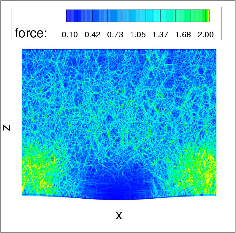
Figure 1: Snapshot of the simulation domain soon after perturbation of the lower boundary has been activated. The figure shows the forces (normalized by the mean) that the particle experience at a given time. The upper wall is static, and the lower one performs standing-wave type of motion. $40,000$ particles.

While the evolution, dynamics, and distribution of force chains is of significant interest in understanding signal propagation in DGM Somfai et al. (2005); Hostler and Brennen (2005), in what follows we consider system quantities which can be averaged over a volume which is small compared to the system size, but which still includes a relatively large number of particles. Furthermore, we also carry out time averaging, choosing an averaging period that is long compared to the particle collision time, but short compared to $1/f$. This averaging procedure is used for calculating the quantities which are later compared to the results of a simple continuum model. The presented results do not depend on the details of the averaging procedure, as long as the general conditions specified above are followed.

In this work, we concentrate on the elastic energy, which is much larger than the kinetic one, to illustrate properties of the propagating signal. Figure 2 shows the elastic energy of the granular particles at several different phases during one period of the boundary oscillation Kondic . We note clear and well-defined wave forms propagating from the lower towards the upper boundary. Analysis of the signal properties such as shown in this figure is one of the main points of this work.

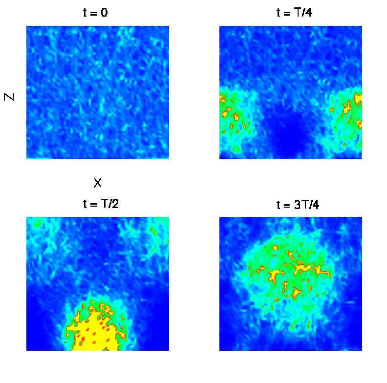
Figure 2: Energy fluctuations for a DEM simulation where a spatially and temporally harmonic perturbation ($\lambda=250d$ and $f=30$ Hz) is applied at the lower boundary (yellow/light corresponds to high energy and blue/dark to low energy). The data in this figure are obtained by subdividing the domain in $64$x$64$ cells and than calculating the cell-averages.

Figure 3 shows the Fourier transforms (FT’s), $E(z;f,\lambda)$, of the elastic energy, $E$, and of the elastic temperature defined as $T=<E>^{2}-<E^{2}>$ associated with the signal Kondic and Behringer (2004). We choose here to present the dominant Fourier mode; the spectral power results are similar. These FT’s are carried out by expanding the energies accumulated during a given time interval in the $x$ direction, and then carrying out a time average over a large number (hundreds or thousands) of periods of the boundary motion. Time averaging serves to increase the signal to noise ratio, and also to ensure that we are not seeing transient effects. The initial results, obtained for the first few periods of the oscillations, are discarded. We have further verified the steady nature of the results by carrying out selected simulations for much longer times.

Figure 3 shows a well defined signal propagating in the $z$-direction. Clearly, $E$ and $T$, which measures local deviations of $E$ from the mean, follow each other closely. Additional simulations show that the system-selected wavelengths in the $z$-direction are independent of the system size Kondic and Behringer . Next we vary $f$ and $\lambda$ of the perturbation, and discuss how the spectrum of the resulting signal changes. We expect that results such as these will be very useful for comparison with any desired continuum model.

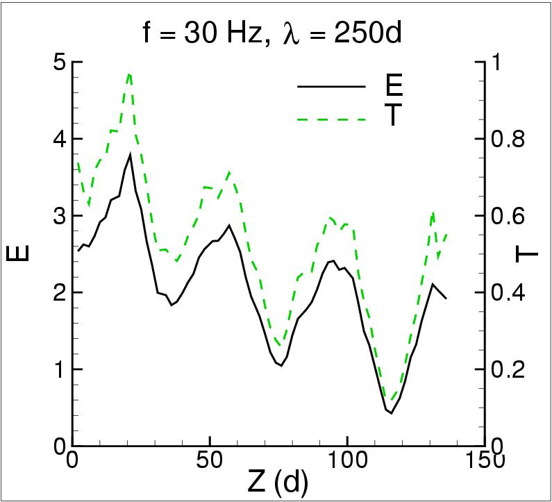
Figure 3: Dominant Fourier mode (the one imposed by the boundary motion) of the elastic energy and temperature as a function of $z$, the distance from the oscillating wall.

Figure 4 shows $E(z;f,\lambda)$ as $\lambda$ and $f$ are varied. In Figs. 4a-b we see that a decrease of $\lambda$ leads to a significant dispersion, that is, the wave-like property of the signal disappears, and the information about the length-scale introduced by the perturbation tends to be lost. Note that although $\lambda$ is decreased, it is still large compared to the particle size. Therefore, we are not in the regime where finite particle size should be important. Figures 4c-d show that an increase of $f$ also leads to the loss of the wave-like signal properties. For a smaller $f$, we see a signal which is weaker and also characterized by a larger $z$-direction wavelength compared to Fig. 3. Therefore, there is just a narrow regime of $f$’s and $\lambda$’s where a well defined signal propagates. For even smaller $f$’s, the energy input is not sufficiently large to be traced in an accurate manner. We note in passing that simulations with an effectively infinite $\lambda$ were also carried out, with the results regarding e.g., the speed of propagation, consistent with the ones in literature Hostler and Brennen (2005).

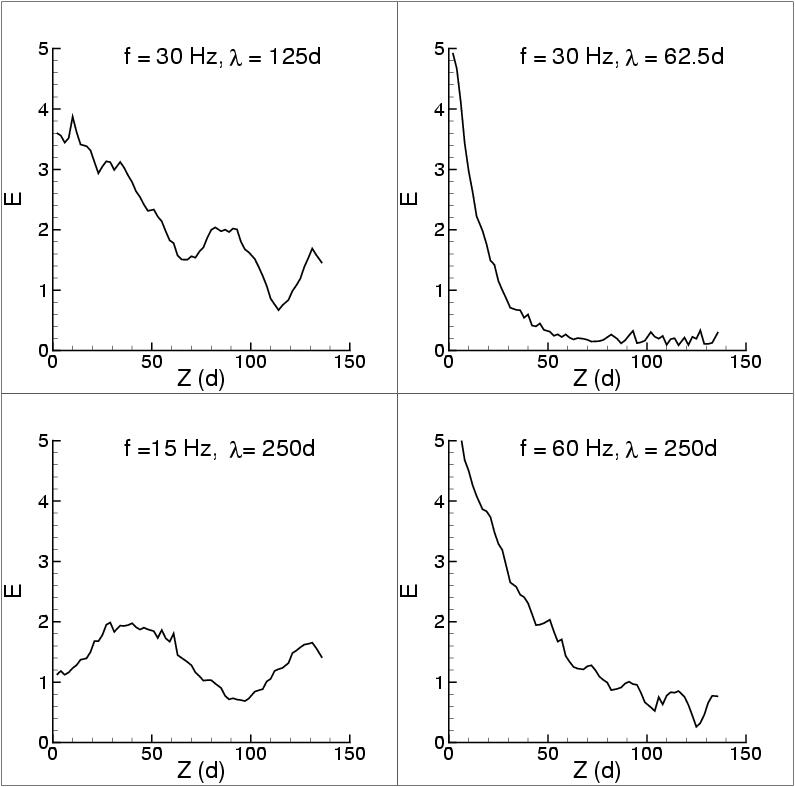
Figure 4: Dominant Fourier mode of the elastic energy as the frequency and wavelength of the perturbation are modified.

We next compare these results to a model which includes elastic behavior and diffusive damping. We chose such a model since static force transmission well above jamming densities is, to date, best described in terms of an elastic picture Goldenberg and Goldhirsch (2005); Geng et al. (2003), and because we anticipate presence of dissipative processes. Assume that the space-time properties of a considered variable $E$ (but similarly for pressure, temperature, or a component of the stress tensor) can be described by

$$\nabla^{2}E-{1\over c^{2}}{\partial^{2}E\over\partial t^{2}}-{1\over D}{\partial E\over\partial t}=0\ ,$$ (1)

which in the limit $D\rightarrow\infty$ reduces to a linear wave equation often used to describe wave propagation in elastic solids, and in the limit $c\rightarrow\infty$ to a diffusion equation, as considered, e.g. in Jia (2004), although for typically much larger $f$’s. We emphasize here that this model in its present form is not meant as a complete description of the simulation results presented so far, but instead as a basis for comparison of signal properties that we understand, and those what we do not.

Eq. (1) is given in a nondimensional form obtained by choosing $L$ as a length scale, and $1/\omega_{p}$ as a time scale, where $\omega_{p}$ is some typical imposed frequency (we use $\omega_{p}=2\pi f_{p}$, $f_{p}=30$ Hz). We take the diffusion $D$, and the speed of propagation, $c$, as constants. Further assuming plane wave solution as a zeroth order approximation to more complex waves that can be expected in DGM Nesterenko (2001); Hostler and Brennen (2005); Sen et al. (2001) in the form $E(x,z,t)=E_{0}e^{\imath\omega t}e^{\imath kx}e^{\imath qz}$, one obtains the following dispersion relation

$$q=-|q|e^{\imath{\phi/2}},\quad|q^{2}|={\cal X}^{2}+({\omega/D})^{2},\quad\tan\phi=-{\omega\over(D{\cal X})}\ ,$$ (2)

where ${\cal X}={(\omega/c)}^{2}-k^{2}$. We first discuss general features of such a mode in light of the simulation results, and note that the results outlined below apply for a wide range of (constant) $c$’s and $D$’s. The following predictions are easily verified: (i) for a fixed frequency of perturbation $f$, an increase of $k$ leads to an increase of the dominant wavelength of the propagating signal, in agreement with Figs. 3 and 4a; (ii) still for a fixed $f$, an increase of $k$ also leads to larger $Im(q)$ showing that stronger attenuation is expected for shorter $\lambda$’s, in agreement with Figs. 3, 4a and 4b; (iii) for a fixed $k$, as $f$ is decreased, one expects longer emerging wavelengths, in agreement with Fig. 4c. We note here that, while the attenuation of a propagating signal as a function of driving frequency has been considered before Jia (2004); Hostler and Brennen (2005), we are not aware of any results discussing the dependence of attenuation on the spatial scales introduced by the perturbation. One feature of the DEM results which is not explained well by the model is the fact that Eq. (1) predicts essentially constant attenuation for larger $f$’s, while in Fig. 4d we see stronger attenuation than e.g. in Fig. 3, consistent with the previous work Jia (2004); Hostler and Brennen (2005). One explanation for this difference is that the model predicts shorter emerging wavelengths for these high frequencies. These shorter wavelengths may become comparable to the particle size, where a continuum model is not expected to apply.

After finding reasonable agreement between the model, Eq. (1), and the simulations, we next ask whether the values of $D$ and $c$ deduced by comparison to the DEM data are in qualitative agreement with the commonly used ones. For this purpose, we extract the value of $q$ from Fig. 3, and using the dispersion relation, Eq. (2), obtain $c\approx 0.025$, $D\approx 0.01$. Similar values of $c$ and $D$ can be extracted from the results shown in Fig. 4 and from additional simulations using other values of $f$ and $\lambda$ (not shown), typically with the spread of obtained values of $D$ larger than the one for $c$. The value of $c$ can now be compared with the speed of sound resulting from elasticity theory, $c*=\sqrt{E_{y}/((1-\sigma^{2})\rho)}/(L\omega_{p})$, where $E_{y},\sigma,\rho$ are the Young modulus, Poisson ratio and density of the material. These material parameters can be extracted from the DEM force model Kondic (1999) (the force constant there corresponds to photoelastic disks such as those used e.g. in Geng et al. (2003)), giving $c/c*\approx 0.1$, in general agreement with other works Somfai et al. (2005).

An interpretation of $D$ is more complicated. An estimate based on the particle size and some typical shear rate, such as average velocity gradient, underestimates significantly the predicted value of $D$, suggesting that a different mechanism is in place. Alternatively, we recall the estimate $D\approx{v_{e}l/3}$ where $v_{e}$ is the velocity of energy transport, and $l$ is the transport mean free path, measuring the distance traveled before the direction of propagation is randomized; for further discussion regarding applicability of this concept to dense granular materials, see, e.g., Sheng (1995); Jia (2004). Let us assume that $v_{e}\approx c*$. The value of $D$ predicted by the model then gives $l$ corresponding to $30-40d$. It will be of interest to analyze whether such a long lengthscale may be related to the correlation length introduced by the force-chain structure, the issue which has been a subject of considerable discussion Liu and Nagel (1992); Jia (2004); Somfai et al. (2005); Hostler and Brennen (2005). It will be also of interest to explore how $l$ (and therefore $D$) vary with, e.g., the volume fraction, or the imposed frequency. An additional task will be to analyze the influence of dimensionality of the system, since it has been suggested that in 3D the correlation length of the force network may be much shorter Jia (2004). We note in passing that, in the regime considered here, a diffusion model that was successfully applied to the 3D system driven at high frequencies Jia (2004), could not explain the main features of the DEM results presented in Figs. 3 and 4.

While we find consistent results between the simulations and the simple continuum model encouraging, we note that much more work is needed. Regarding simulations, we have considered propagation for a given volume fraction, therefore not considering explicitly the pressure dependence of the speed of propagation. For smaller volume fractions (closer to the jamming threshold) the nature of the signal propagation may be modified, and it remains to be seen how the continuum model used here would apply in that case. Regarding the continuum model itself, although we find that it describes well many features of the DEM results, better understanding of the attenuation properties of the signal is needed. The degree of agreement with the simulations suggests that for more precise comparison one may need to consider frequency-dependent $D$. The question of coupling of different spacial and temporal scales needs to be considered as well.

We hope that probing DGM with both space and time dependent perturbations, as done here, will be utilized in future theoretical and particularly experimental efforts to build a more complete picture regarding stress and energy transport in dense granular matter.

Acknowledgments We thank Joe Goddard for useful comments. This work was supported by NSF Grants No. DMS 0605857 and DMR 0555431.

References

- Coppersmith et al. (1996) S. N. Coppersmith et al., Phys. Rev. E 53, 4673 (1996).
- Otto et al. (2003) M. Otto et al., Phys. Rev. E 67, 0313023 (2003).
- Bouchaud et al. (1994) J. P. Bouchaud et al., J. Phys. I France 4, 1383 (1994).
- Blumenfeld (2004) R. Blumenfeld, Phys. Rev. Lett. 93, 108301 (2004).
- Goldenberg and Goldhirsch (2005) C. Goldenberg and I. Goldhirsch, Nature 435, 188 (2005).
- Nedderman (1992) R. M. Nedderman, Statics and kinematics of granular materials (Cambridge University Press, 1992).
- Goddard (1990) J. D. Goddard, Proc. R. Soc. Lond. A 430, 105 (1990).
- Geng et al. (2003) J. Geng et al., Physica D 182, 274 (2003).
- Sheng (1995) P. Sheng, Introduction to Wave Scattering, Localization, and Mesoscopic Phenomena (Academic Press, 1995).
- Liu and Nagel (1992) C.-h. Liu and S. R. Nagel, Phys. Rev. Lett. 68, 2301 (1992).
- Makse et al. (1999) H. A. Makse et al., Phys. Rev. Lett. 83, 5070 (1999).
- Jia (2004) X. Jia, Phys. Rev. Lett. 93, 154303 (2004).
- Somfai et al. (2005) E. Somfai et al., Phys. Rev. E 72, 021301 (2005).
- Hostler and Brennen (2005) S. R. Hostler and C. E. Brennen, Phys. Rev. E 72, 031303 (2005).
- Nesterenko (2001) V. Nesterenko, Dynamics of Heterogenous Materials (Springer, New York, 2001).
- Kondic (1999) L. Kondic, Phys. Rev. E 60, 751 (1999).
- Johnson (1989) K. L. Johnson, Contact Mechanics (Cambridge University Press, Cambridge, 1989).
- (18) L. Kondic and R. P. Behringer, in preparation.
- (19) L. Kondic, http://m.njit.edu/~kondic/granular/signal/signal.html.
- Kondic and Behringer (2004) L. Kondic and R. P. Behringer, Europhys. Lett. 67, 205 (2004).
- Sen et al. (2001) S. Sen et al., Granular Matter 3, 33 (2001).