Quantum Accelerator Modes near Higher-Order Resonances.

Abstract

Quantum Accelerator Modes have been experimentally observed, and theoretically explained, in the dynamics of kicked cold atoms in the presence of gravity, when the kicking period is close to a half- integer multiple of the Talbot time. We generalize the theory to the case when the kicking period is sufficiently close to any rational multiple of the Talbot time, and thus predict new rich families of experimentally observable Quantum Accelerator Modes.

Present-day experimental techniques afford almost perfect control of the state and time evolution of quantum systems, and thus allow observation of phenomena, that are rooted in subtle aspects of the quantum-classical correspondence. In particular, effects of mode-locking and nonlinear resonance, that are ubiquitous in classical nonlinear dynamics, could be observed on the quantum level, in the form of unexpected quantum stabilization phenomena; for instance, in nondispersive wave-packet dynamics MNG05 , and in the kicked dynamics of cold and ultra-cold atoms. In the latter case, techniques originally introduced by M. Raizen and coworkers have been successfully used to produce atom-optical realizations of the Kicked Rotor (KR) model KR , which is a famous paradigmatic model of Quantum Chaos. A variant of the KR, which was realized in Oxford, had the (Cesium) atoms freely falling under the effect of gravity between kicks. Discovery of a new effect followed, which was named Quantum Accelerator Modes (QAM) Ox99 . A natural internal time scale for the system is set by the so-called Talbot time, and whenever the kicking period is close to a half-integer multiple of that time, small groups of atoms are observed to steadily accelerate away from the bulk of the atomic cloud, at a rate and in a direction (upwards, or downwards) which depend on parameter values. A theory for this phenomenon FGR03 introduces a dimensionless parameter $\epsilon$, which measures the detuning from exact resonance, and shows that the nearly resonant quantum dynamics may be obtained from quantization of a certain classical dynamical system , using $\epsilon$ as the Planck’s constant. This dynamical system was termed the $\epsilon$-classical limit of the quantum dynamics, and is quite different from the system, which is obtained in the classical limit proper $\hbar\to 0$. QAM are absent in the latter limit, and are accounted for by $\epsilon$-classical phase space structures. Thus, they are at once a purely quantal phenomenon, and a manifestation of classical nonlinear resonance; indeed, their theory is a repertory of classic items of nonlinear dynamics, occurring in a purely quantum context. For instance, they are associated with Arnol’d tongues in the space of parameters, and are hierarchically organized according to number-theoretical rules farey . Finally, on the quantum level, a deep relation to the famous problem of Bloch oscillations and Wannier-Stark resonances WS has been exposed SFGR06 .
Existence of QAM somehow related to other rational multiples of the Talbot time (”higher order resonances”), than just the half-integer ones, is a long-standing question, that lies beyond the reach of the existing theory. Some indications in this sense are given by numerical simulations, and also by generalizations of heuristic arguments GS , which were formerly devised Ox99 in order to explain the first experimental observations of QAM.
In this paper we show that QAM indeed exist near resonances of arbitrary order. This noticeable re-assessment of the QAM phenomenon requires a nontrivial reformulation of the small-$\epsilon$ approximation, in order to circumvent the basic difficulty, that no $\epsilon$-classical limit exists in the case of higher resonances. We show that, in spite of that, families of rays (in the sense of geometrical optics) nonetheless exist, that give rise to QAM in the vicinity of a KR resonance. Such ”accelerator rays” are not trajectories of a single formally classical system, but rather come in families, generated by different classical systems, which provide but local (in phase space) approximations to the quantum dynamics. This is remindful of the small-$\hbar$ asymptotics for the dynamics of particles, in the presence of spin-orbit interactions LF91 . This similarity is by no means accidental, because the KR dynamics at higher-order resonance may be described in terms of spinors IS80 ; SZAC ; thus, the present problem naturally fits into a more general theoretical framework, and our formal approach may find application in the broader context of quantum kicked dynamics, in the presence of spin.
The dynamics of kicked atoms moving in the vertical direction under the effect of gravity is modeled by the following time-dependent Hamiltonian:

$${\hat{H}}(t)\;=\;\frac{1}{2}({\hat{P}}+\frac{\eta}{\tau}t)^{2}\;+\;kV({\hat{X}})\;\sum_{n=-\infty}^{+\infty}\delta(t-n\tau)\;.$$ (1)

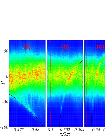
Figure 1: (Color online) Momentum distributions, in the time dependent gauge, after $n=100$ kicks, for different values of the kicking period near the resonance $\tau=\pi$ ((a) and (b)), and near the resonance $\tau=14\pi/13$ (c). Red color corresponds to highest probability. The initial state is a mixture of 100 plane waves sampled from a gaussian distribution of momenta. Vertical dashed lines correspond to the mentioned resonant values of $\tau/2\pi$. Black full lines show the theoretical curves (12), with: (a) $T=2,{\mathfrak{p}}=3,{\mathfrak{j}}=1,\Delta_{2}=0$ , (b) $T=1,{\mathfrak{p}}=5,{\mathfrak{j}}=1,\Delta_{1}=0$ and (c) $T=1,{\mathfrak{p}}=5,{\mathfrak{j}}=1,\Delta_{1}=20\pi/13$. Parameter values are: $k=0.8\pi$ and $\eta=0.126\tau$.

Units are chosen so that the atomic mass is 1, Planck’s constant is 1, and the spatial period of the kicks is $2\pi$. The dimensionless parameters $k,\tau,\eta$ are expressed in terms of the physical parameters as follows: $k=\kappa/\hbar$, $\tau=\hbar TG^{2}/M$, $\eta=MgT/(\hbar G)$, where $M,T,\kappa$ are the atomic mass, the kicking period, the kick strength, and $2\pi/G$ is the spatial period of the kicks. $\hat{X}$ is the position operator (along the vertical direction) and the kicking potential $V({\hat{X}})=\cos({\hat{X}})$ in experiments. Hamiltonian (1) is written in a special, time dependent gauge FGR03 , in which the canonical momentum operator is given by ${\hat{P}}+\eta t/\tau$. This choice of a gauge makes (1) invariant under spatial translations by $2\pi$, so, by Bloch theory, the quasi-momentum $\beta$ is conserved. With the present units, $\beta$ is the fractional part of $\hat{P}$. The dynamics at fixed $\beta$ are formally those of a rotor with angular coordinate $\theta=X$mod$(2\pi)$. Let $|\psi_{n}\rangle$ denote the state of the rotor immediately after the $n$-th kick; then $|\psi_{n+1}\rangle={\hat{U}}_{n}|\psi_{n}\rangle$, where the unitary operators ${\hat{U}}_{n}$ are given, in the $\theta$-representation, by:

$${\hat{U}}_{n}\;=\;e^{-ikV({\theta})}\;e^{-i\frac{\tau}{2}(-i\partial_{\theta}+\beta+\eta/2+\eta n)^{2}}\;.$$ (2)

For $\eta=0$, ${\hat{U}}_{n}$ does not depend on $n$, and coincides with the propagator of the generalized Kicked Rotor. Multiplication of wavefunctions $\psi(\theta)$ by $\exp(im\theta)$, ($m\in{\mathbb{Z}}$) generates the discrete unitary group of (angular) momentum translations. For special values of $\tau$ and $\beta$ a nontrivial subgroup of such translations commutes with the KR propagator. This leads to a special dynamical behaviour, called KR-resonance IS80 . We define the order of a KR resonance as the minimum index of a commuting subgroup; or, the least positive integer $\ell$ such that (2) commutes with multiplication by $\exp(i\ell\theta)$. KR resonances occur if, and only if refwhen , $\tau$ is commensurate to $2\pi$, and the quasi-momentum $\beta$ is rational. Indeed, momentum translations by multiples of an integer $\ell$ leave (2) invariant if, and only if, (i) $\tau=2\pi p/q$ with $p,q$ coprime integers, (ii) $\ell=mq$ for some integer $m$, and (iii) $\beta={\nu}/mp+mq/2$ mod$(1)$, with $\nu$ an arbitrary integer. In the following we restrict to ”primary” resonances, which have $m=1$ and $\ell=q$, and generically denote $\beta_{r}$ the resonant values of quasi-momentum. The KR propagator at exact resonance is obtained on substituting $\tau=2\pi p/q$, $\beta=\beta_{r}$, and $\eta=0$ in (2). Using Poisson’s summation formula, it may be written in the form:

$${\hat{U}}_{\mbox{\rm\tiny res}}\psi(\theta)\;=\;e^{-ikV(\theta)}\sum\limits_{s=0}^{q-1}G_{s}\;{\psi}(\theta-2\pi s/q)\;,$$ (3)

where

$$G_{s}\equiv G_{s}(p,q,\beta_{r})\;=\;\frac{1}{q}\sum\limits_{l=0}^{q-1}e^{-\pi ip(l+\beta_{r})^{2}/q}\;e^{2\pi isl/q}\;,$$ (4)

so that $|G_{s}|=q^{-1/2}$. Now let $\tau=2p\pi/q+\epsilon$, $\beta=\beta_{r}+\delta\beta$; and denote $\phi_{n}=\delta\beta+\eta/2+\eta n$. We may write

$${\hat{U}}_{n}\;=\;{\hat{U}}_{\mbox{\rm\tiny res}}\exp(-i\frac{\epsilon}{2}(-i\partial_{\theta}+\beta_{r})^{2})\;\exp(-\tau\phi_{n}\partial_{\theta})\;.$$ (5)

Here, and in the following, phase factors only dependent on $\beta$ and $n$ are disregarded. Thanks to eqn.(3), eqn.(5) may be rewritten in the following form :

$$({\hat{U}}_{n}\psi)(\theta)\;=\;e^{-ikV(\theta)}\sum\limits_{s=0}^{q-1}\;G_{s}\;{\tilde{\psi}}(\theta-2\pi s/q-\tau\phi_{n})\;,$$ (6)

where:

$${\tilde{\psi}}(\theta)\;=\;e^{-i\frac{\epsilon}{2}(-i\partial_{\theta}+\beta_{r})^{2}}\psi(\theta)\;.$$ (7)

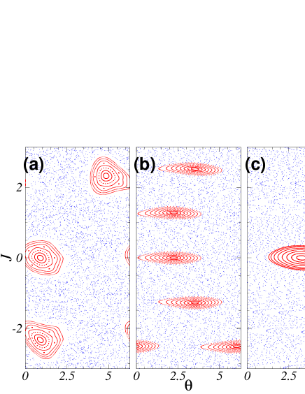
Figure 2: (Color online) Phase portraits of maps ${\cal F}^{(T)}_{0}$ on the 2-torus, for (a) $T=2,\delta_{s}=(-1)^{s+1}\pi,\tilde{k}=-0.395,\tau\eta=1.122,({\mathfrak{p}},{\mathfrak{j}})=(3,1)$ $(\tau/2\pi=0.475,\epsilon=-0.157)$; (b) $T=1,\delta_{s}=0,\tilde{k}=0.032,\tau\eta=1.253,({\mathfrak{p}},{\mathfrak{j}})=(5,1)$ $(\tau/2\pi=0.502,\epsilon=0.013)$ and (c) $T=1,\delta_{s}=20\pi/13,\tilde{k}=0.040,\tau\eta=1.455,({\mathfrak{p}},{\mathfrak{j}})=(1,1)$ $(\tau/2\pi=0.541,\epsilon=0.016)$.

If $\epsilon$ is granted the formal role of Planck’s constant, then operator (7) has the form of a unitary propagator for a generalized free rotor SH , so quasi-classical methods may be used to investigate the small-$\epsilon$ regime. We define the $\epsilon$-classical momentum operator ${\hat{I}}=-i\epsilon\partial/\partial\theta$ . Denoting ${\tilde{k}}\equiv k\epsilon$, the $\epsilon$-quasiclassical asymptotic regime is defined by $\epsilon\to 0$ at constant ${\tilde{k}},I$. Using the explicit form of the integral kernel for (7) SH , the transition amplitude from $\theta=\theta_{0}$ at time $0$ to $\theta=\theta_{n}$ after $n$ kicks is given by:

$$\langle\theta_{n}|{\hat{U}}_{n-1}\ldots{\hat{U}}_{0}|\theta_{0}\rangle=(2\pi i\epsilon)^{-n/2}\sum\limits_{({\bf m},{\bf s})\in\Omega_{n}}G_{s_{0}}\ldots G_{s_{n-1}}\times$$

$$\times\int_{0}^{2\pi}\ldots\int_{0}^{2\pi}d\theta_{1}\ldots d\theta_{n-1}e^{i\epsilon^{-1}S_{{\bf m},{\bf s}}(\theta_{0},\theta_{1},\ldots,\theta_{n})}\;,$$ (8)

where ${\bf m}$ and ${\bf s}$ are vectors with $(n-1)$ integer components, $\Omega_{n}\equiv{\mathbb{Z}}^{n-1}\times\{1,\ldots,q\}^{n-1}$, and

$$S_{{\bf m},{\bf s}}(\theta_{0},\ldots,\theta_{n})=\sum\limits_{t=1}^{n}\{-{\tilde{k}}V(\theta_{t})+$$

$$+\frac{1}{2}(\theta_{t}-\theta_{t-1}-2\pi s_{t}/q-2m_{t}\pi-\tau\phi_{t})^{2}\}\;.$$ (9)

Replacing (9) in (8), and using the stationary phase approximation in individual terms in the sum on the rhs of (8), we find that, at small $|\epsilon|$, (7) propagates along rays, which satisfy the equations :

$$\theta_{t+1}\; = \;\theta_{t}\;+\;I_{t}\;+\;\tau\phi_{t}\;+2\pi s_{t}/q\;\mbox{\rm mod}\;2\pi$$

$$I_{t+1}\; = \;I_{t}\;-\;{\tilde{k}}V^{\prime}(\theta_{t+1})\;,$$ (10)

or, defining $J_{t}\equiv I_{t}+\tau\phi_{t}+2\pi s_{t}/q$, and $\delta_{t}\equiv 2\pi(s_{t+1}-s_{t})/q$,

$$J_{t+1}\; = \;J_{t}\;+\delta_{t}+\tau\eta-{\tilde{k}}\;V^{\prime}(\theta_{t+1})\;,$$

$$\theta_{t+1}\; = \;\theta_{t}\;+J_{t}\;\mbox{\rm mod}(2\pi)\;.$$ (11)

For each value of $t$, (Quantum Accelerator Modes near Higher-Order Resonances.) defines a map ${\cal F}_{t}$ on the cylinder; however, since the choice of the integers $s_{1},s_{2},\ldots$ is totally arbitrary whenever $q>1$, such maps do not, in general, uniquely define a classical dynamical system. The $s_{t}$ may be removed by changing variables to $\vartheta=q\theta$, but this calls into play the function $V^{\prime}(\vartheta/q)$, which is not a single-valued function in $\vartheta\in[0,2\pi]$, except in the case when $V(\theta)$ is a $2\pi/q$-periodic function; then eqs. (Quantum Accelerator Modes near Higher-Order Resonances.) reduce to a single map, and the theory proceeds essentially identical as in the case $q=1$. In all other cases, exponentially many different maps enter the game upon iterating eqs.(Quantum Accelerator Modes near Higher-Order Resonances.), and so no $\epsilon$-classical limit proper exists. In spite of that, we shall presently show how a stability requirement singles out special families of rays, which give distinguished contributions in the dynamics, ultimately resulting in QAM. In stationary phase approximation, each ray (Quantum Accelerator Modes near Higher-Order Resonances.) contributes a term $q^{-n/2}|$det$({\mathfrak{M}})|^{-1/2}\exp(iS_{{\bf s},{\bf m}}/\epsilon+i\Phi_{\bf s})$ in (8), where $S_{{\bf s},{\bf m}}$ is the action (9) computed along the given ray, $\Phi_{\bf s}$ collects phases from the $G_{s_{t}}$ and from Maslov indices, and $\mathfrak{M}$ is the matrix of 2nd derivatives of (9) with respect to the angles $\theta_{1},\ldots,\theta_{n-1}$. Stability of a ray is related to the behavior of the prefactor $|$det$({\mathfrak{M}})|^{-1/2}$ as a function of ”time” $n$. $\mathfrak{M}$ is a tridiagonal Jacobi matrix, with off-diagonal elements equal to $-1$, and diagonal elements given by $-{\tilde{k}}V^{\prime\prime}(\theta_{t})+2$, where $\theta_{t}$ are the angles along the ray. For a large number $n$ of kicks, most choices of ${\bf s}\in\{1,\ldots,q\}^{n}$ are essentially random. The same may be assumed to be true of the diagonal elements of $\mathfrak{M}$, and so $\mathfrak{M}$ has a positive Lyapunov exponent, due to Anderson localization. It follows that $|$det$({\mathfrak{M}})|$ exponentially increases with $n$ (as may be seen, e.g., from the Herbert-Jones-Thouless formula PF ). Therefore, such rays carry exponentially small contributions, and their global effect is determined by interference of exponentially many such contributions. In contrast, distinguished contributions are given by those rays, whose matrices $\mathfrak{M}$ have extended states, thanks to absence of diagonal disorder. The simplest such case occurs when the diagonal elements of $\mathfrak{M}$ are a periodic sequence. This in particular happens when $\delta_{t}$ is a periodic sequence, and rays are in such cases related to stable periodic orbits of certain classical dynamical systems, which are constructed as follows. Let $\delta_{t+T}=\delta_{t}$ for some $T$ and all $t$. Then map ${\cal F}_{t}$ (Quantum Accelerator Modes near Higher-Order Resonances.) periodically depends on ”time” $t$; so, for each choice of $t^{\prime}$ with $0\leq t^{\prime}<T-1$, one may introduce a ”map over one period” ${\cal F}^{(T)}_{t^{\prime}}\equiv{\cal F}_{t^{\prime}+T-1}\circ\ldots\circ{\cal F}_{t^{\prime}}$, whose iteration determines rays (Quantum Accelerator Modes near Higher-Order Resonances.) at every $T$-th kick after the $t^{\prime}$-th one. As this map is $2\pi$-periodic in $J,\theta$, it defines a dynamical system on the 2-torus. Systems that way constructed with different $t^{\prime}$ are obviously conjugate to each other, so the periodic orbits of any of them one-to-one correspond to the periodic orbits that are obtained for $t^{\prime}=0$. As a result, to each periodic orbit of ${\cal F}^{(T)}_{0}$ (on the 2-torus) a ray (Quantum Accelerator Modes near Higher-Order Resonances.) is associated, which is periodic in position space; therefore, its matrix $\mathfrak{M}$ has periodic diagonal elements. If the orbit has period $\mathfrak{p}$, then the corresponding ray (Quantum Accelerator Modes near Higher-Order Resonances.) satisfies $J_{(l+{\mathfrak{p}})T}=J_{lT}+2\pi{\mathfrak{j}}$ for all integer $l$, where $\mathfrak{j}$ is the ”jumping index” of the periodic orbit. This is equivalent to $I_{(l+{\mathfrak{p}})T}=I_{lT}-2\pi(s_{(l+{\mathfrak{p}})T}-s_{lT})/q-\tau\eta T{\mathfrak{p}}+2\pi{\mathfrak{j}}$ and so, along such a ray, the physical momentum $I/\epsilon$ linearly increases (or decreases) with average acceleration

$$a=\epsilon^{-1}\left\{2\pi{\mathfrak{j}}({\mathfrak{p}}T)^{-1}-\Delta_{T}-\tau\eta\right\}\;,$$ (12)

where $\Delta_{T}=T^{-1}\sum_{s=0}^{T-1}\delta_{s}$. Finally, stability of such rays, as determined by the behavior of det$({\mathfrak{M}})$ as a function of ”time” $n$, is controlled by the Lyapunov exponent, and so is equivalent to dynamical stability of the corresponding periodic orbits .
In summary: whenever $V(\theta)$ is not $2\pi/q$-periodic, no $\epsilon$-classical limit exists for the dynamics (8); QAM may nevertheless exist, associated with stable ”accelerator rays”, that are associated with the stable periodic orbits of a family of maps of the 2-torus. There is one such map for each choice of a periodic sequence in $\{1,\ldots,q\}^{{\mathbb{N}}}$. The simplest choice is $\delta_{t}=0$ ; the relevant map (Quantum Accelerator Modes near Higher-Order Resonances.), and the acceleration formula (12), are then the same as in the case $q=1$ FGR03 . In Fig. 1 we show numerical evidence for QAM associated with the resonances at $q=2$, $p=1$ ((a) and (b)) and at $q=13$, $p=7$ (c). Here, the kicking potential is $V(\theta)=\cos(\theta)$. For the given parameter values, three QAM are clearly detected: two around the $q=2$, $p=1$ resonance, one near the $q=13$, $p=7$ one. They correspond, via eq. (12), to stable periodic orbits of maps ${\cal F}^{(T)}_{0}$ with $T=1$ and with $T=2$. The stable islands of these orbits are shown in Fig. 2.
The present theory suggests an unsuspected richness of QAM, associated with the dense set of higher-order resonances. If produced with ideal, infinite resolution, figures in the style of Fig. 1 might reveal that QAM are essentially ubiquitous; however, some QAM associated with resonances of low order $q>1$ should be observable already on the present level of experimental resolution. Our numerical simulations have exposed a fine texture of seemingly QAM-like structures; on the available level of precision, however, most of them are so vague, that it is impossible to decide to which resonance they belong. Those for which this question could be answered were in all cases found to correspond to some stable orbits, in agreement with the above theory. On the other hand, for a few of the periodic orbits we have computed, no partner QAM could be detected. This may be due to the fact that, at given parameter values, many different orbits coexist, which are related to different resonances, hence to different values of the pseudo-Planck constant $\epsilon$. The hierarchical rules that determine their relative ”visibility” are not known at this stage. In general, one may expect stronger QAM near lower order resonances, yet exceptions are not rare, see Fig.1 (c).

We thank G. Summy for communicating results obtained by his group, prior to publication, and S. Fishman for his constant attention and precious comments in the course of this work.

References

- (1) H.Maeda, D.V.L.Norum, T.F.Gallagher, Science 307, 1757, (2005); F.B. Dunning et al., Adv. At. Mol. Opt. Phys 52, 49, (2005).
- (2) F. L. Moore, J. C. Robinson,C. F. Bharucha, B. Sundaram, and M. G. Raizen, Phys.Rev.Lett. 75, 4598, (1995); H. Amman, R. Gray, I. Shvarchuck, N. Christensen, Phys. Rev. Lett. 80, 4111, (1998); P. Szriftgiser, J. Ringot, D. Delande, J.C. Garreau, Phys. Rev. Lett. 89, 22410, (2002); C. Ryu, M.F. Andersen, A. Vaziri, M.B. d’Arcy, J.M. Grossmann, K. Helmerson, W.D. Phillips, Phys. Rev. Lett. 96, 1604031, (2006).
- (3) M.K. Oberthaler, R.M. Godun, M.B. d’Arcy, G.S. Summy and K. Burnett, Phys.Rev.Lett. 83, 4447, (1999); R.M. Godun, M.B. d’Arcy, M.K. Oberthaler, G.S. Summy, and K. Burnett, Phys. Rev. A 62, 013411, (2000); S. Schlunk, M.B. d’Arcy, S.A. Gardiner, G.S. Summy, Phys. Rev. Lett. 90, 124102, (2003).
- (4) S. Fishman, I. Guarneri, and L.Rebuzzini, J. Stat. Phys. 110, 911, (2003); Phys. Rev. Lett. 89, 084101, (2002) .
- (5) A. Buchleitner, M.B. d’Arcy, S. Fishman, S.A. Gardiner, I. Guarneri, Z.Y. Ma, L. Rebuzzini, G.S. Summy, Phys. Rev. Lett. 96, 164101, (2006); I. Guarneri, L. Rebuzzini and S. Fishman, Nonlinearity 19, 1141, (2006); R.Hihinashvili,T.Oliker,Y.S. Avizrats,A. Jomin, S.Fishman, I.Guarneri , Physica D 226, 1, (2007).
- (6) M. Gluck, A. Kolovsky, H.J. Korsch Phys. Rep. 366, 103, (2002).
- (7) M. Sheinman, S. Fishman, I. Guarneri, L. Rebuzzini, Phys. Rev. A 73, 052110, (2006).
- (8) F.M. Izrailev and D.L. Shepelyansky, Theor. Mat. Phys. 43, 353, (1980); G. Casati and I.Guarneri, Comm.Math. Phys. 95 121, (1984); F.M. Izrailev, Phys. Rep. 196, 299, (1990).
- (9) G. Summy, private communication.
- (10) R.G. Littlejohn and W.G. Flynn, Phys. Rev. A 44, 5239, (1991).
- (11) V.V. Sokolov, O.V. Zhirov, D. Alonso, and G. Casati, Phys. Rev. Lett. 84, 3566, (2000); Phys. Rev. E 61, 5057, (2000).
- (12) I.Dana and D.L.Dorofeev, Phys. Rev. E 73, 026206, (2006).
- (13) L.S. Schulman, Techniques and Applications of Path Integration, Wiley 1996, p.190.
- (14) D.J. Thouless, J.Phys. C 5, 77, (1972); D.C.Herbert and R.Jones, ibidem 4, 1145, (1971).