Characterizing Long-Period Transiting Planets Observed by Kepler

Abstract

Kepler will monitor a sufficient number of stars that it is likely to detect single transits of planets with periods longer than the mission lifetime. We show that by combining the exquisite Kepler photometry of such transits with precise radial velocity observations taken over a reasonable timescale ($\sim 6$ months) after the transits, and assuming circular orbits, it is possible to estimate the periods of these transiting planets to better than 20%, for planets with radii greater than that of Neptune, and the masses to within a factor of 2, for planets with masses larger than or about equal to the mass of Jupiter. Using a Fisher matrix analysis, we derive analytic estimates for the uncertainties in the velocity of the planet and the acceleration of the star at the time of transit, which we then use to derive the uncertainties for the planet mass, radius, period, semimajor axis, and orbital inclination. Finally, we explore the impact of orbital eccentricity on the estimates of these quantities.

1 Introduction

Planets that transit their stars offer us the opportunity to study the physics of planetary atmospheres and interiors, which may help constrain theories of planet formation. From the photometric light curve, we can measure the planetary radius and also the orbital inclination, which when combined with radial velocity (RV) observations, allows us to measure the mass and density of the planet. Infrared observations of planets during secondary eclipse can be used to measure the planet’s thermal spectrum (Charbonneau et al., 2005; Deming et al., 2005), and spectroscopic observations around the time of transit can constrain the composition of the planet’s atmosphere through transmission spectroscopy (Charbonneau et al., 2002). Additionally, optical observations of the secondary eclipse can probe a planet’s albedo (Rowe et al., 2007). All of the known transiting planets are Hot Jupiters or Hot Neptunes, which orbit so close to their parent stars that the stellar flux plays a major role in heating these planets. In contrast, the detection of transiting planets with longer periods ($P>1\,{\rm yr}$) and consequently lower equilibrium temperatures, would allow us to probe a completely different regime of stellar insolation, one more like that of Jupiter and Saturn whose energy budgets are dominated by their internal heat.

Currently, it is not feasible to find long-period, transiting planets from the ground. While RV surveys have found $\sim 110$ planets with periods $\gtrsim 1\,{\rm yr}$, it is unlikely that any of these transit their parent star, given that for a solar-type host, the transit probability is very small, $\wp_{\rm tr}\simeq 0.5\%(P/{\rm yr})^{-2/3}$. Thus the sample of long-period planets detected by RV will need to at least double before a transiting planet is expected. Given the long lead time necessary to detect long-period planets with RV observations, this is unlikely to happen in the near future. Furthermore, the expected transit times for long-period systems are relatively uncertain, which makes the coordination and execution of photometric follow-up observations difficult. Putting all this together, radial velocity surveys are clearly an inefficient means to search for long-period, transiting planets.

Ground-based photometric transit surveys are similarly problematic. A long-period system must be monitored for a long time because typically, at least two transits must be observed in order to measure the period of the system. Furthermore, if there are a couple of days of bad weather at the wrong time, the transit event will be missed entirely, rendering years of data worthless. Thus transit surveys for long-period planets require many years of nearly uninterrupted observations. Additionally, many thousands of suitable stars must be monitored to find a single favorably-inclined system.

Because of its long mission lifetime ($L=3.5\,{\rm yrs}$), nearly continuous observations, and large number of target stars ($N\simeq 10^{5}$), the Kepler satellite (Borucki et al., 2004; Basri et al., 2005) has a unique opportunity to discover long-period transiting systems. Not only will Kepler observe multiple transits of planets with periods up to the mission lifetime, but it is also likely to observe single transits of planets with periods longer than the mission lifetime. As the period of a system increases beyond $L/2$, the probability of observing more than one transit decreases until, for periods longer $L$, only one transit will ever be observed. For periods longer than $L$, the probability of seeing a single transit diminishes as $P^{-5/3}$. Even with only a single transit observation from Kepler, these long-period planets are invaluable.

We show that planets with periods longer than the mission lifetime will likely be detected and can be characterized using the Kepler photometry and precise radial velocity observations. Furthermore, this technique can be applied to planets that will transit more than once during the Kepler mission, so that targeted increases in the time-sampling rate can be made at the times of subsequent transits.

In $\S$2 we calculate the number of one- and two-transit systems Kepler is expected to observe. We give a general overview of how the Kepler photometry and radial velocity follow-up observations can be combined to characterize a planet in $\S$3. We discuss in $\S$4 the expected uncertainties in the light curve observables, and we relate these to uncertainties in physical quantities, such as the period, that can be derived from the transit light curve. $\S$5 describes the expected uncertainties associated with the RV curve and how they influence the uncertainty in the mass of the planet. $\S$6 discusses the potential impact of eccentricity on the ability to characterize long-period planets. We summarize our conclusions in $\S$7. Details of the derivations are reserved for an appendix ($\S$8).

2 Expected Number of Planets

The number of single-transit events Kepler can expect to find is the integral of the probability that a given system will be favorably inclined to produce a transit, multiplied by the probability that a transit will occur during the mission, convolved with a distribution of semimajor axes, and normalized by the expected frequency of planets and the number of stars that Kepler will observe,

$$N_{\rm tot}=N_{\star}\int\wp_{\rm tr}\wp_{L}f(a)da.$$ (1)

Here $N_{\rm tot}$ is the total number of transiting systems expected, $N_{\star}$ is the number of stars being monitored, $\wp_{\rm tr}$ is the probability that the system is favorably inclined to produce a transit (the transit probability), $\wp_{L}$ is the probability that a transit will occur during the mission, and $f(a)$ is some distribution of the planet semimajor axis $a$, normalized to the expected frequency of planets.

Assuming a circular orbit, the transit probability is simply,

$$\wp_{\rm tr}=\frac{R_{\star}}{a}=\left(\frac{4\pi^{2}}{G}\right)^{1/3}M_{\star}^{-1/3}R_{\star}P^{-2/3},$$ (2)

where $R_{\star}$ and $M_{\star}$ are the radius and mass of the parent star, and $P$ is the period of the system.

We consider both the probability of observing exactly one transit, $\wp_{L,1}$, and the probability of observing exactly two transits, $\wp_{L,2}$. These probabilities are

$$\wp_{L,1}=\left\{\begin{array}[]{ll}\frac{2P}{L}-1&\frac{L}{2}\leq P\leq L,\\ \frac{L}{P}&P\geq L.\end{array}\right.$$ (3)

$$\wp_{L,2}=\left\{\begin{array}[]{ll}\frac{4P}{L}-1&\frac{L}{4}\leq P\leq\frac{L}{2},\\ 2-\frac{2P}{L}&\frac{L}{2}\leq P\leq L.\end{array}\right.$$ (4)

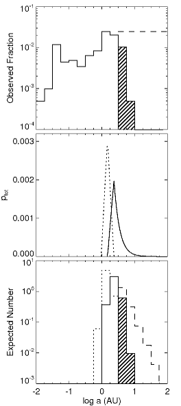
Thus there will be a range in periods from $L/2$ to $L$ where it is possible to get either one or two transits during the mission. If we assume a mission lifetime of $L=3.5$ years and a solar-type star ($R_{\star}=R_{\odot},M_{\star}=M_{\odot}$), we can find the total probability ($\wp_{\rm tr}\wp_{L}$) of observing a planet that transits and exhibits exactly one or exactly two transits as a function of period or semimajor axis. These probability distributions as functions of $a$ are shown in the middle panel of Fig. 1.

For $P\geq L$, the total probability, $\wp_{\rm tot}$, of observing a single transit is

$$\wp_{\rm tot}\equiv\wp_{\rm tr}\wp_{L}=0.002\left(\frac{R_{\star}}{R_{\odot}}\right)\left(\frac{M_{\star}}{M_{\odot}}\right)^{-1/3}\left(\frac{P}{3.5{\rm\,yrs}}\right)^{-5/3}\left(\frac{L}{3.5{\rm\,yrs}}\right).$$ (5)

Thus the probability that the planet will transit and that a single transit will occur during the mission is generally small for periods at the mission lifetime, and beyond this is a strongly decreasing function of the period, $\propto P^{-5/3}$ or $\propto a^{-5/2}$.

The observed distribution of semimajor axes for planets with minimum masses $m_{\rm p}\sin i\geq 0.3~{}M_{\rm Jup}$ is shown in the top panel of Figure 1, where $m_{\rm p}$ is the mass of the planet, $i$ is the orbital inclination, and the data are taken from the “Catalog of Nearby Exoplanets” of Butler et al. (2006). Note that we have included multiple-planet systems. We normalized the distribution by assuming that 8.5% of all stars have planets with $m_{\rm p}\sin i\geq 0.3~{}M_{\rm Jup}$ and $a\leq 3~{}{\rm AU}$ (Cumming et al., 2008). We can extrapolate this distribution to larger semimajor axes by observing that it is approximately constant as a function of $\log a$ and adopting the value found by Cumming et al. (2008), $dN/d\log{a}=4.3\%$. Using this extrapolation, we predict $13.4\%$ and $16.4\%$ of stars have a $m_{\rm p}\sin i\geq 0.3~{}M_{\rm Jup}$ planet within $10~{}{\rm AU}$ and $20~{}{\rm AU}$, respectively, in agreement with Cumming et al. (2008).

We find the number of planets expected for Kepler by convolving this normalized distribution with the probability distribution and multiplying by $N_{\star}=100,000$. We convolve the distribution of semimajor axes with the total transit probability distribution by weighting the probability of observing a transit for each member of the bin to determine an overall probability for the bin. The bottom panel of Fig. 1 shows the resulting distribution of one- and two-transit systems. Integrating this distribution over all semimajor axes out to the limit of current RV observations predicts that Kepler will observe a total of 4.0 single-transit systems and 5.6 two-transit systems during the mission lifetime of $L=3.5\,{\rm yrs}$. If we include the extrapolation of the observed distribution to larger semimajor axes, the integrated number of single-transit systems increases to 5.7; the effect is modest because the probability of observing a transit declines rapidly with increasing semimajor axis ($\wp_{\rm tot}\propto a^{-5/2}$).

Thus, Kepler is likely to detect at least handful of single-transit events. It is important to bear in mind that this is a lower limit. First, our estimate does not include planets with $m_{\rm p}\sin i\lesssim 0.3~{}M_{\rm Jup}$, primarily because RV surveys are substantially incomplete for low-mass, long-period planets. As we will show, Kepler will be able to constrain the periods of planets with radii as small as that of Neptune with the detection of a single transit. Indeed, microlensing surveys indicate that cool, Neptune-mass planets are common (Beaulieu et al., 2006; Gould et al., 2006). Second, Barnes (2007) and Burke (2008) showed that a distribution in eccentricity increases the probability that a planet will transit its parent star. Finally, if the Kepler survey lifetime is extended, the number of detections of long-period transiting planets will also increase.

One might assume that a single-transit event must simply be discarded from the sample because the event is not confirmed by a second transit, and the period cannot be constrained by the time between successive transits. Although we do not expect to see many of them, long-period transiting planets are precious, as the information we could potentially gain by observing these systems when they transit in the future would allow us to greatly enhance our understanding of the physical properties of outer giant planets, and in particular would allow us to compare them directly to our own solar system giants. Thus, these single transit events should be saved, if at all possible.

Figure 1: (top) The observed distribution of semimajor axes for planets with minimum masses $m_{\rm p}\sin i\geq 0.3~{}M_{\rm Jup}$. The shaded region indicates $a\geq 10^{0.5}\,\mathrm{AU}\approx 3\,{\rm AU}$, where we expect the sample to suffer from incompleteness. The dashed line indicates our extrapolation of the distribution, found by assuming the constant distribution in $\log a$ from Cumming et al. (2008). (middle) The total transit probability. The solid line shows the probability that a planet transits and exhibits a single transit during the Kepler mission lifetime. The dotted line shows the same probability for two transits. (bottom) The expected number of one and two-transit events. The probability distribution has been convolved with the observed fraction of planets and multiplied by the number of stars Kepler will observe (100,000) to give the number of single transit systems (solid line) and two transit systems (dotted line) that can be expected. The dashed line shows the convolution of the single transit probability distribution with the extrapolation to larger semimajor axes.

3 Characterizing a Planet

With a few basic assumptions, Kepler photometry of a transiting planet can provide a period for the system that can be combined with precise radial velocity measurements to estimate a mass for the planet. Here we briefly sketch the basics of how these properties can be estimated and what their uncertainties are, and we provide details in the following sections. We assume the planet is much less massive than the star, $m_{\rm p}\ll M_{\star}$, and circular orbits. We consider the impact of eccentricity on our conclusions in §6.

Assuming no limb-darkening and assuming the out-of-transit flux is known perfectly, a transit can be characterized by four observables, namely the fractional depth of the transit $\delta$, the full-width half-maximum of the transit $T$, the ingress/egress duration $\tau$, and the time of the center of transit $t_{c}$. These can be combined to estimate the instantaneous velocity of the planet at the time of transit,

$$v_{\rm tr,p}=2R_{\star}\left(\frac{\sqrt{\delta}}{T\tau}\right)^{1/2}.$$ (6)

For a circular orbit, $v_{\rm tr,p}$ can be used to estimate the period of the planet

$$P=\frac{2\pi a}{v_{\rm tr,p}}=\frac{G\pi^{2}}{3}\rho_{\star}\left(\frac{T\tau}{\sqrt{\delta}}\right)^{3/2},$$ (7)

where we have employed Kepler’s third law assuming that the planet’s mass is much smaller than the star’s mass. Thus, if the stellar density $\rho_{\star}$ is known, then the planet’s period can be estimated from photometry of a single transit (Seager & Mallén-Ornelas, 2003). Note that there is a degeneracy between $\rho_{\star}$ and $P$, so with a single transit $\rho_{\star}$ must be determined by other means in order to derive an estimate of $P$. $\rho_{\star}$ can be estimated via spectroscopy combined with theoretical isochrones, or asteroseismology. The total uncertainty in the period is the quadrature sum of the contribution from the estimate of $\rho_{\star}$ and the contribution from the Kepler photometry (i.e., the uncertainty at fixed $\rho_{\star}$),

$$\left(\frac{\sigma_{P}}{P}\right)_{\rm tot}^{2}=\left(\frac{\sigma_{\rho_{\star}}}{\rho_{\star}}\right)^{2}+\left(\frac{\sigma_{P}}{P}\right)_{\rm Kep}^{2}.$$ (8)

The contribution from Kepler is dominated by the uncertainty in the ingress/egress time $\tau$,

$$\left(\frac{\sigma_{P}}{P}\right)_{\rm Kep}^{2}\approx\frac{9}{4}\left(\frac{\sigma_{\tau}}{\tau}\right)^{2}\approx Q^{-2}\left(\frac{27T}{2\tau}\right),$$ (9)

where we have assumed $\tau\ll T$, and that the number of points taken out of transit is much larger than the number taken during the transit (and thus the out-of-transit flux is known essentially perfectly). Here $Q$ is approximately equal to the total signal-to-noise ratio of the transit,

$$Q\equiv(\Gamma_{\rm ph}T)^{1/2}\delta,$$ (10)

where $\Gamma_{\rm ph}$ is the photon collection rate. For Kepler we assume,

$$\Gamma_{\rm ph}=7.8\times 10^{8}~{}{\rm hr^{-1}}\,10^{-0.4(V-12)},$$ (11)

and thus Kepler will detect a single transit with a signal-to-noise ratio of

$$Q\simeq 1300\,\left(\frac{R_{\star}}{R_{\odot}}\right)^{-3/2}\left(\frac{M_{\star}}{M_{\odot}}\right)^{-1/6}\left(\frac{r_{\rm p}}{R_{\rm Jup}}\right)^{2}\left(\frac{P}{3.5{\rm\,yrs}}\right)^{1/6}10^{-0.2(V-12)},$$ (12)

where $r_{\rm p}$ is the radius of the planet. For a Neptune-size planet with these fiducial parameters, $Q\simeq 150$.

Kepler’s contribution to the uncertainty in the period is,

$$\left(\frac{\sigma_{P}}{P}\right)_{\rm Kep}^{2}=7.7\times 10^{-5}10^{0.4(m_{v}-12)}\left(\frac{R_{\star}}{R_{\odot}}\right)^{4}\left(\frac{M_{\star}}{M_{\odot}}\right)^{1/3}\left(\frac{R_{\rm Jup}}{r_{\rm p}}\right)^{5}\left(\frac{3.5{\rm\,yrs}}{P}\right)^{1/3},$$ (13)

where we have assumed the impact parameter $b=0$. Due to the strong scaling with $r_{\rm p}$ and relatively weak scaling with $P$, there are essentially two regimes. For $r_{\rm p}\gtrsim R_{\rm Nep}$, the uncertainty in $P$ is dominated by uncertainties in the estimate of $\rho_{\star}$, which is expected to be ${\cal O}(10\%)$, whereas for $r_{\rm p}<R_{\rm Nep}$, it is very difficult to estimate the period due to the uncertainty in $\tau$ from the Kepler photometry.

Once the period is known from the photometry, the mass of the planet, $m_{\rm p}$, can be measured with radial velocity observations. For a circular orbit, and for observations spread out over a time that is short compared to $P$, the radial velocity of the star can be expanded about the time of transit, and so approximated by the velocity at the time of transit $v_{0}$, plus a constant acceleration $A_{\star}$,

$$v_{\star}\approx v_{0}-A_{\star}(t-t_{c}),$$ (14)

where $A_{\star}=2\pi K_{\star}/P$, and

$$K_{\star}=\left(\frac{2\pi G}{PM_{\star}^{2}}\right)^{1/3}m_{\rm p}\sin i$$ (15)

is the stellar radial velocity semi-amplitude. Thus,

$$m_{\rm p}=A_{\star}\left(\frac{M_{\star}^{2}}{G}\right)^{1/3}\left(\frac{P}{2\pi}\right)^{4/3}=\frac{1}{16G}g_{\star}^{2}A_{\star}\left(\frac{T\tau}{\sqrt{\delta}}\right)^{2},$$ (16)

where $g_{\star}$ is the surface gravity of the star, and we have assumed $\sin\,i=1$.

The uncertainty in the planet mass has contributions from three distinct sources: the uncertainty in $g_{\star}$, which can be estimated from spectroscopy, the uncertainty in $A_{\star}$, which is derived from RV observations after the transit, and the uncertainties in $T,\,\tau,$ and $\delta$, which are derived from Kepler photometry. In fact, the uncertainty in $\tau$ dominates over the uncertainties in $T$ and $\delta$. Therefore, we may write,

$$\left(\frac{\sigma_{m_{\rm p}}}{m_{\rm p}}\right)^{2}=4\left(\frac{\sigma_{g_{\star}}}{g_{\star}}\right)^{2}+\left(\frac{\sigma_{A_{\star}}}{A_{\star}}\right)^{2}+4\left(\frac{\sigma_{\tau}}{\tau}\right)^{2}.$$ (17)

For reasonable assumptions and long-period planets ($P\gtrsim 1~{}{\rm yr}$), we find that the uncertainty in $A_{\star}$ dominates over the uncertainty in $\tau$.

Assuming that $N$ equally-spaced RV measurements with precision $\sigma_{\rm RV}$ are taken over a time period $T_{\rm tot}$ after the transit, the uncertainty in $A_{\star}$ is,

$$\left(\frac{\sigma_{A_{\star}}}{A_{\star}}\right)^{2} \simeq \frac{12\sigma_{\rm RV}^{2}}{A_{\star}^{2}T_{\rm tot}^{2}N},$$ (18)

$$\simeq 0.85\left(\frac{\sigma_{\rm RV}}{10{\rm\,m\,s}^{-1}}\right)^{2}\left(\frac{3{\rm\,mos}}{T_{\rm tot}}\right)^{2}\left(\frac{20}{N}\right)\left(\frac{M_{\rm Jup}}{m_{\rm p}}\right)^{2}\left(\frac{M_{\star}}{M_{\odot}}\right)^{4/3}\left(\frac{P}{3.5{\rm\,yrs}}\right)^{8/3},$$

where we have assumed $N\gg 1$. Thus, radial velocity observations combined with Kepler photometry can confirm the planetary nature of a Jupiter-sized planet in a relatively short time span. An accurate ($\lesssim 10\%$) measurement of the mass for a Jupiter-mass planet, or even a rough characterization of the mass for a Neptune-mass planet, will require either more measurements, or measurements with substantially higher RV precision. Of course, additional radial velocity observations over a time span comparable to $P$ will further constrain the mass and period.

In $\S$4 and $\S$5, we derive the above expressions for the uncertainty in the mass and the period of the planet using a Fisher information analysis.

4 Estimating the Uncertainty in P

4.1 Uncertainties in the Light Curve Observables

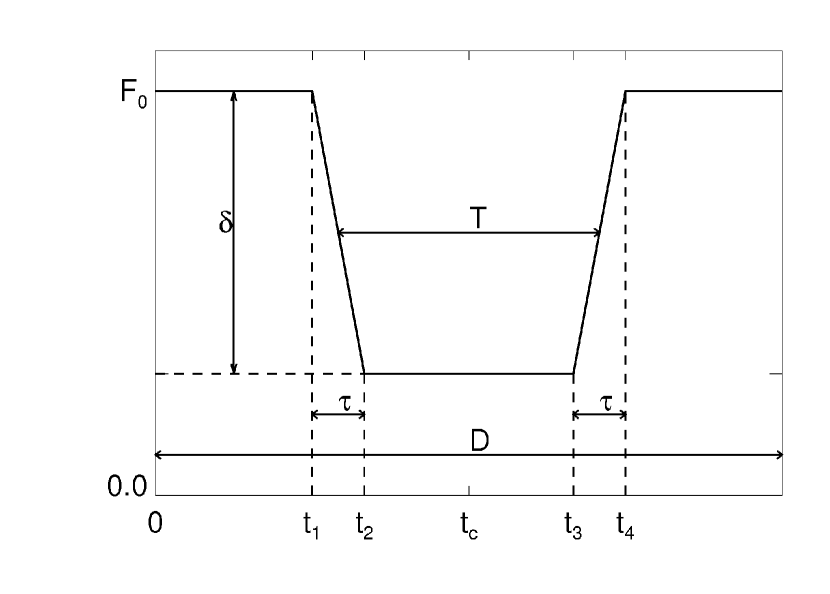
In the absence of significant limb-darkening, a transit light curve can be approximated by a trapezoid that is described by the five parameters $t_{c}$, $T$, $\tau$, $\delta$, and $F_{0}$, where $F_{0}$ is the out-of-transit flux. Figure 2 shows this simple trapezoidal model and labels the relevant parameters. Mathematically, the flux $F$ as a function of time $t$ is given by,

$$F(t)=\left\{\begin{array}[]{ll}F_{0},&t<t_{1},\\ F_{0}-\delta(t-[t_{c}-T/2-\tau/2])/\tau,&t_{1}\leq t\leq t_{2},\\ F_{0}-\delta,&t_{2}<t<t_{3},\\ F_{0}-\delta(1-[(t-[t_{c}-T/2-\tau/2])/\tau]),&t_{3}\leq t\leq t_{4},\\ F_{0},&t_{4}<t,\end{array}\right.$$ (19)

where $t_{1}$ – $t_{4}$ are the points of contact. We also define $D$ to be the total duration of the observations. This model is fully differentiable and can be used with the Fisher matrix formalism to derive exact expressions for the uncertainties in the parameters $t_{c}$, $T$, $\tau$, $\delta$, and $F_{0}$. We note that the definition for $\delta$ we use here differs slightly from the definition we adopted in §3. Here $\delta$ is the depth of the transit (e.g., in units of flux), rather than the fractional depth. These two definitions differ by a factor of $F_{0}$ such that $\delta_{frac}=\delta_{flux}/F_{0}$. However, when $D\gg T$ (as will be the case for Kepler), the uncertainty in $F_{0}$ is negligible, and so one may define $F_{0}=1$, thus making these two parametrizations equivalent.

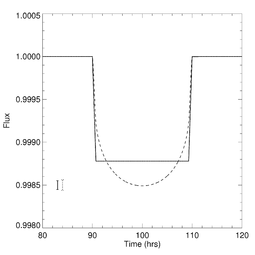
Figure 3 compares this simple model with the exact model computed using the formalism of Mandel & Agol (2002), in this case for a transit of the Sun by Neptune with a 3.5-year period and an impact parameter of $b=0.2$. We see that the trapezoidal model provides an excellent approximation to the exact light curve, and as we will show the analytic parameter uncertainties are quite accurate. We also show the case of significant limb-darkening as expected for a Sun-like star observed in the R-band (similar to the Kepler bandpass). In this case, the match is considerably poorer, but nevertheless we will show the analytic parameter uncertainties we derive assuming the simple trapezoidal model still provide useful estimates (see Carter et al. 2008 for a more thorough discussion).

We derive exact expressions for the uncertainties in $t_{c}$, $T$, $\tau$, $\delta$, and $F_{0}$ by applying the Fisher matrix formalism to the simple light curve model (a detailed explanation of the Fisher matrix is given by Gould 2003). The full details of the derivation are given in the appendix ($\S$8). In the case of the long-period transiting planets that will be observed by Kepler, we can simplify the full expression by making a couple of assumptions. We assume that the flux out of transit, $F_{0}$, is known to infinite precision and that $\tau\ll T\ll D$. The uncertainties in the remaining parameters are,

$$\sigma_{t_{c}} =Q^{-1}\sqrt{\frac{T\tau}{2}},$$ (20)

$$\frac{\sigma_{T}}{T} =Q^{-1}\sqrt{\frac{2\tau}{T}},$$ (21)

$$\frac{\sigma_{\tau}}{\tau} =Q^{-1}\sqrt{\frac{6T}{\tau}},$$ (22)

$$\frac{\sigma_{\delta}}{\delta} =Q^{-1}.$$ (23)

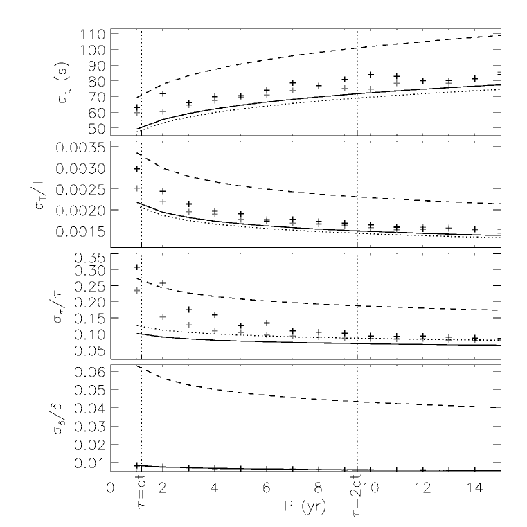
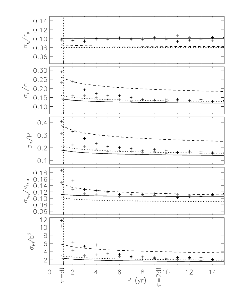
We tested the accuracy of these expressions using Monte Carlo simulations. We generate 1000 light curves for a given set of orbital parameters. We assume that the planet orbits a solar-type star in a circular orbit with an impact parameter of 0.2. We repeat the analysis for four of the solar-system planets: Jupiter, Saturn, Neptune, and Earth. We assume the expected photometric precision for Kepler for a stellar apparent magnitude of $V=12$ (a representative magnitude for Kepler’s stellar sample), a sampling rate of one per $30\,\mathrm{min}$, and a total duration for the observations of $D=200$ hours. Then we fit for the parameters $t_{c}$, $T$, $\tau$, $\delta$, and $F_{0}$ using a down-hill simplex method. The uncertainty in each parameter is taken to be the standard deviation in the distribution of the fits for that parameter. A comparison of the analytic expressions and the Monte Carlo simulations is shown in Fig. 4, where we have plotted the uncertainties as a function of period for a planet with radius $1R_{\rm Nep}$ crossing a star with radius $1R_{\odot}$ at an impact parameter $b=0.2$. We find that the Fisher matrix approximation breaks down as the number of points during ingress/egress becomes small.

We also considered expected uncertainties for the exact uniform source and limb-darkened models for the transit light curve. Mandel & Agol (2002) give the full solution for a transit involving two spherical bodies and provide code for calculating the transit light curve. They also include a limb-darkened solution. These models may be parametrized by the same observables described in our simplified model. The full and limb-darkened light curves are plotted in Fig. 3 as the dotted and dashed curves, respectively. We use the limb-darkening coefficients from Claret (2000) closest to observations of the Sun ($T_{\rm eff}=5750~{}{\rm K}$, $\log(g_{\star})=4.5~{}{\rm\,cm\,s}^{-1}$, $[M/H]=0.0$) in the R-band. We apply the Fisher matrix method to numerical derivatives of these model light curves to compare the uncertainties for the full and limb-darkened solutions with the analytic uncertainties for the trapezoidal model. A comparison of the uncertainties from the different models is shown in Fig. 4. We find that the simplified model is a good approximation for the exact, uniform-source transit model. While the comparison is less favorable with the limb-darkening model, the uncertainties do not differ by more than a factor of a few.

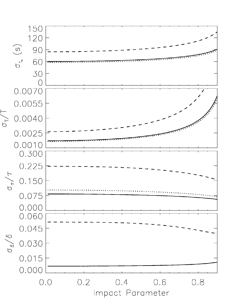
We also compared how the uncertainties in the transit observables varied with impact parameter $b$ for the three models, because varying $b$ will affect the relative sizes of $T$ and $\tau$. These comparisons are shown in Fig. 5 for Neptune in a circular orbit around the Sun with a 3.5-year period. As can be seen from the figure, variations in $b$ have little impact in the uncertainties in the observables for $b\lesssim 0.8$.

Figure 2: The simplified model of a transit light curve showing the points of contact ($t_{1},t_{2},t_{3},t_{4}$), the transit depth ($\delta$), the ingress/egress time ($\tau$), the FWHM duration of the transit ($T$), the total duration of observations ($D$), and the time of the transit center ($t_{c}$).

Figure 3: Three different models of a transit light curve. The solid line shows the simplified trapezoidal model, the dotted line (barely visible) shows the exact, uniform-source light curve, and the dashed line includes the effects of limb-darkening. The exact uniform-source and limb-darkened light curves are calculated using Mandel & Agol (2002). These light curves were generated for a Neptune analog orbiting a solar analog at a period of $P=3.5~{}{\rm yrs}$ and an impact parameter $b=0.2$. Typical error bars for Kepler assuming $V=12.0$ and 30-min sampling (solid) or 20-min sampling (dotted) are indicated.

Figure 4: Uncertainty in observables as a function of period. The uncertainties in $t_{c}$, $T$, $\tau$, and $\delta$ are plotted versus period for Neptune orbiting the Sun with an impact parameter of 0.2. The different line styles indicate the trapezoidal transit model (solid line), the full solution (dotted line), and a model including the effects of limb-darkening (dashed line). Monte-Carlo simulations of the trapezoidal model using 30-minute sampling are shown as crosses. The gray crosses show simulations for 20-minute sampling. The dotted line in the bottom panel is not visible because it is nearly identical to the solid line. The vertical dotted lines mark where the ingress/egress duration $\tau$ is equal to the sampling rate $dt$, as well as where $\tau=2dt$ for 30-minute sampling.

Figure 5: Uncertainty in observables as a function of impact parameter. The uncertainties in $t_{c}$, $T$, $\tau$, and $\delta$ are plotted versus impact parameter for Neptune orbiting the Sun with a period of 3.5 years. The line styles are the same as for Fig. 4. As in Fig. 4, the dotted line in the bottom panel is not visible because it is nearly identical to the solid line.

4.2 Uncertainties in Quantities Derived From the Light Curve

Assuming the planet is in a circular orbit, and assuming the stellar density, $\rho_{\star}$, is estimated from independent information, Seager & Mallén-Ornelas (2003) demonstrated that the planet period, $P$, and impact parameter, $b$, can derived from a single observed transit, with sufficiently precise photometry. In fact, provided independent estimates of $M_{\star}$ and $R_{\star}$ are available, then it is also possible to derive the planet radius, $r_{p}$, semimajor axis, $a$, and instantaneous velocity at the time of transit, $v_{\rm tr,p}$.

The uncertainties in these physical parameters can be calculated through standard error propagation. Equations for these quantities and their uncertainties are given in Eqs. 24–28 (Note that we calculate $b^{2}$ instead of $b$ because numerical methods have difficulty when $T\sqrt{\delta}/\tau\approx 1$). In each case below, the second approximate uncertainty equation is calculated by substituting the variances and covariances of the observables $\tau,\,T$, and $\delta$, and simplifying under the assumption that $\tau\ll T\ll D$.

$$r_{\rm p} = R_{\star}\sqrt{\delta}$$ (24)

$$\sigma_{r_{\rm p}}^{2} = r_{\rm p}^{2}\left(\frac{1}{R_{\star}}\sigma_{R_{\star}}^{2}+\frac{1}{4\delta^{2}}\sigma_{\delta}^{2}\right)$$

$$\simeq r_{\rm p}^{2}\left(\frac{1}{R_{\star}}\sigma_{R_{\star}}^{2}+\frac{1}{4}Q^{-2}\right)$$

$$b^{2} = 1-\frac{T\sqrt{\delta}}{\tau}$$ (25)

$$\sigma_{b^{2}}^{2} = \left[\frac{\delta}{\tau^{2}}\sigma_{T}^{2}+\frac{T^{2}\delta}{\tau^{4}}\sigma_{\tau}^{2}+\frac{T^{2}}{4\tau^{2}\delta}\sigma_{\delta}^{2}-\frac{2T\delta}{\tau^{3}}\sigma_{T\tau}^{2}+\frac{T}{\tau^{2}}\sigma_{T\delta}^{2}-\frac{T^{2}}{\tau^{3}}\sigma_{\tau\delta}^{2}\right]$$

$$\simeq T\delta Q^{-2}\left(\frac{6T^{2}}{\tau^{3}}\right)$$

$$a = \frac{g_{\star}}{4}\left(\frac{T\tau}{\sqrt{\delta}}\right)$$ (26)

$$\sigma_{a}^{2} = a^{2}\left[\frac{1}{g_{\star}^{2}}\sigma_{g_{\star}}^{2}+\frac{1}{T^{2}}\sigma_{T}^{2}+\frac{1}{\tau^{2}}\sigma_{\tau}^{2}+\frac{1}{4\delta^{2}}\sigma_{\delta}^{2}+\frac{2}{T\tau}\sigma_{T\tau}^{2}-\frac{1}{T\delta}\sigma_{T\delta}^{2}-\frac{1}{\tau\delta}\sigma_{\tau\delta}^{2}\right]$$

$$\simeq a^{2}\left[\frac{1}{g_{\star}^{2}}\sigma_{g_{\star}}^{2}+Q^{-2}\left(\frac{6T}{\tau}\right)\right]$$

$$v_{\rm tr,p} = 2R_{\star}\left(\frac{\sqrt{\delta}}{T\tau}\right)^{1/2}$$ (27)

$$\sigma_{v_{\rm tr,p}}^{2} = v_{\rm tr,p}^{2}\left[\frac{1}{R_{\star}^{2}}\sigma_{R_{\star}}^{2}+\frac{1}{4T^{2}}\sigma_{T}^{2}+\frac{1}{4\tau^{2}}\sigma_{\tau}^{2}+\frac{1}{16\delta^{2}}\sigma_{\delta}^{2}+\frac{1}{2T\tau}\sigma_{T\tau}^{2}-\frac{1}{4T\delta}\sigma_{T\delta}^{2}-\frac{1}{4\tau\delta}\sigma_{\tau\delta}^{2}\right]$$

$$\simeq v_{\rm tr,p}^{2}\left[\frac{1}{R_{\star}^{2}}\sigma_{R_{\star}}^{2}+Q^{-2}\left(\frac{3T}{2\tau}\right)\right]$$

$$P = \frac{\pi G}{4}\left(\frac{4}{3}\pi\rho_{\star}\right)\left(\frac{T\tau}{\sqrt{\delta}}\right)^{\frac{3}{2}}$$ (28)

$$\sigma_{P}^{2} = P^{2}\left[\frac{1}{\rho^{2}_{\star}}\sigma_{\rho_{\star}}^{2}+\frac{9}{4T^{2}}\sigma_{T}^{2}+\frac{9}{4\tau^{2}}\sigma_{\tau}^{2}+\frac{9}{16\delta^{2}}\sigma_{\delta}^{2}+\frac{9}{2T\tau}\sigma_{T\tau}^{2}-\frac{9}{4T\delta}\sigma_{T\delta}^{2}-\frac{9}{4\tau\delta}\sigma_{\tau\delta}^{2}\right]$$

$$\simeq P^{2}\left[\frac{1}{\rho^{2}_{\star}}\sigma_{\rho_{\star}}^{2}+Q^{-2}\left(\frac{27T}{2\tau}\right)\right]$$

Of course, the quantities $R_{\star}$, $g_{\star}$, and $\rho_{\star}$ and their uncertainties must be estimated from some other external source of information, such as spectroscopy or theoretical isochrones. We can generally expect that the fractional uncertainties on these quantities will be of order $10\%$. For long-period ($P\gtrsim L=3.5~{}{\rm yrs}$), Jupiter-sized planets, $Q\gg 1$, and thus the variances and covariances of the transit observables will be small in comparison to the expected uncertainties on $R_{\star},\rho_{\star}$, and $g_{\star}$.

The fractional uncertainties in these derived parameters are plotted in Fig. 6. We compared the analytic uncertainties given in Eqs. 24–28 to the Monte Carlo simulations described in Sec. 4.1. The fractional uncertainty in each parameter from the Monte Carlo simulations is one-half the range of the middle 68% of the data divided by the median. Notice that as $\tau$ decreases from $2dt$ to $dt$, the simulations become increasingly disparate from the theoretical expectations. $\sigma_{r_{\rm p}}/r_{\rm p}$ does not show this behavior because it does not depend on $\tau$. In this regime, as $\tau$ decreases, it becomes increasingly probable that only one point will be taken during ingress leaving $\tau$ relatively unconstrained and increasing its uncertainty and the uncertainty of quantities that depend on it.

We now consider in detail the uncertainty in the estimated period. Given that $Q\propto T^{1/2}\delta$, we have that $Q^{-2}(T/\tau)\propto(\delta^{2}\tau)^{-1}$. Since $\tau\propto r_{\rm p}P^{1/3}$ and $\delta\propto r_{\rm p}^{2}$, the contribution to the uncertainty in the period due to the Kepler photometry is a much stronger function of the planet’s radius than its period, $Q^{-2}(27T/2\tau)\propto r_{\rm p}^{-5}P^{-1/3}$. As a result, for a fixed stellar radius $R_{\star}$, the ability to accurately estimate $P$ depends almost entirely on $r_{\rm p}$. Furthermore, because the scaling with $r_{\rm p}$ is so strong, there are essentially two distinct regimes: for large $r_{\rm p}$, the uncertainty in $P$ is dominated by the uncertainty in $\rho_{\star}$, whereas for small $r_{\rm p}$, the period cannot be estimated. The boundary between these two regimes is where the contribution to the uncertainty in the period from $\rho_{\star}$ is equal to the contribution from the Kepler photometry, i.e. where the two terms in the brackets in Eq. 28 are equal. This occurs at a radius of,

$$r_{\rm p,crit}\simeq R_{\rm Nep}\left[10^{0.4(V-12)}\left(\frac{\sigma_{\rho_{\star}}/\rho_{\star}}{0.1}\right)^{-2}\left(\frac{R_{\star}}{R_{\odot}}\right)^{4}\left(\frac{M_{\star}}{M_{\odot}}\right)^{1/3}\left(\frac{3.5{\rm\,yrs}}{P}\right)^{1/3}\right]^{1/5},$$ (29)

assuming $b=0$. Note that $r_{\rm p,crit}$ is a weak or extremely weak function of all of the parameters except $R_{\star}$.

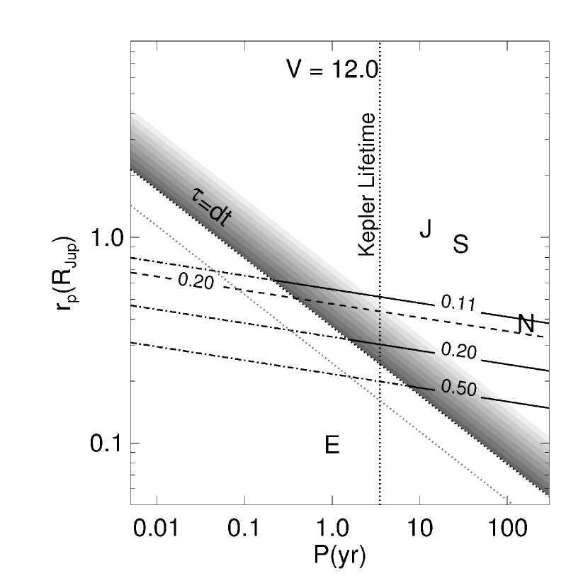
Fig. 7 illustrates this point by showing contours of constant uncertainty in the period as a function of the radius and period of the planet. The calculations are for systems with $R_{\star}=R_{\odot}$, $b=0.2$, and $V=12.0$. This figure shows that for planets larger than the radius of Neptune, the uncertainty in the period will be dominated by the uncertainty in the inferred stellar density, whereas for planets much smaller than Neptune, an accurate estimate of the period from the Kepler light curve will be impossible.

As shown above, the uncertainty in $P$ is dominated by the uncertainty in $\rho_{\star}$ and $\tau$. Our ability to determine $\tau$, and its uncertainty, depends both on its length and how many points we have during the ingress or egress. The length of $\tau$ depends on $v_{\rm tr,p}$ (which is a proxy for $P$ in the circular case), $b$, and $r_{\rm p}$. These properties are intrinsic to the system, but may be derived from the observables. We can explore how the contours shown in Fig. 7 vary with impact parameter. Figure 5 shows that a system with a larger impact parameter will have a smaller fractional uncertainty in $\tau$. Thus, a system with a larger impact parameter would have a smaller fractional uncertainty in $P$ at fixed period and planet radius.

The other effect that influences the contours is the sampling of $\tau$. As the number of points taken during the ingress/egress becomes small, the fractional uncertainty in $\tau$, and hence in $P$, increases. In particular, if only one point is taken during the ingress, then the duration is relatively unconstrained. The probability of taking only one point during the ingress increases linearly from 0 to 1 as $\tau$ decreases from $2dt$ to $dt$. In Fig. 6, the Monte Carlo simulations for the fractional uncertainty in $P$ diverge from the simple model over this range. We indicate this region by the shaded portion of Fig. 7. Where $\tau=dt$, the fractional uncertainty in $P$ can be several times that predicted by the theoretical calculations, but these uncertainties converge as the shading gets lighter towards $\tau=2dt$. Below the line where $\tau=dt$, the uncertainty in $\tau$ increases rapidly, but fortunately, in much of this regime, Kepler will observe multiple transits, and this analysis will be unnecessary. As shown in the figure, a faster sampling rate, such as 1 per 20 min, significantly expands the parameter space over which our theoretical uncertainties are valid.

Figure 6: Uncertainty in derived quantities as a function of period. The uncertainties in $r_{\rm p}$, $a$, $P$, $v_{\rm tr,p}$, and $b^{2}$ are plotted versus period for Neptune orbiting the Sun with an impact parameter of 0.2. The line styles are the same as for Fig. 4. The vertical dotted lines mark where the ingress/egress duration $\tau$ is equal to the sampling rate $dt$, as well as where $\tau=2dt$ for 30-minute sampling.

Figure 7: Contours of constant fractional uncertainty in the period as a function of the period and the planet radius. The model is for a solar-type star with a V magnitude of 12.0 and an impact parameter for the system of 0.2. The dashed line indicates how the fractional uncertainty in $P$ changes with $V$ magnitude; it shows the 0.20 contour for $V=14.0$ and $b=0.2$. The diagonal black dotted line represents the boundary below which the assumptions of Fisher matrix break down (the ingress/egress time $\tau$ is roughly equal to the sampling rate of 1/30 min). Thus, the contours below this boundary are shown as dash-dotted lines. The region between $\tau=2dt$ and $\tau=dt$ is shaded to indicate the increasingly probability of obtaining only one point during ingress or egress leading to an uncertainty in $P$ that is larger than theoretical expectations. The diagonal gray dotted line indicates the $\tau=dt$ boundary for 20-min sampling. The vertical dotted line shows the mission lifetime of Kepler ($L=3.5\,{\rm yrs}$). Solar system planets are indicated.

5 Estimating the Uncertainty in $m_{\rm p}$

The mass of the planet comes from sampling the stellar radial velocity curve soon after the transit is observed. Near the time of transit we can expand the stellar radial velocity,

$$v_{\star}=v_{0}-K_{\star}\sin\left[\frac{2\pi}{P}(t-t_{c})\right]\approx v_{0}-A_{\star}(t-t_{c}),$$ (30)

where $v_{0}$ is the systemic velocity, $K_{\star}$ is the stellar radial velocity semi-amplitude, and $A_{\star}\equiv 2\pi K_{\star}/P$ is the stellar acceleration. Because the planet is known to transit and has a long period, we assume $\sin i=1$. A Fisher matrix analysis of the linear form of Eq. 30 gives the estimated uncertainty in $A_{\star}$ to be

$$\sigma_{A_{\star}}^{2}\simeq\frac{12\sigma_{\rm RV}^{2}}{T_{\rm tot}^{2}N},$$ (31)

where $\sigma_{\rm RV}$ is the radial velocity precision, $T_{\rm tot}$ is the total time span of the radial velocity observations, and $N$ is the number of observations, and we have assumed $N\gg 1$ and that the observations are evenly spaced in time. The details of this derivation are given in the appendix ($\S$8).

Equations for the mass of the planet and the uncertainty are

$$m_{\rm p} = \frac{1}{16G}g_{\star}^{2}A_{\star}\left(\frac{T\tau}{\sqrt{\delta}}\right)^{2}$$ (32)

$$\sigma_{m_{\rm p}}^{2} = m_{\rm p}^{2}\left[\frac{4}{g_{\star}^{2}}\sigma_{g_{\star}}^{2}+\frac{1}{A_{\star}^{2}}\sigma_{A_{\star}}^{2}+\frac{4}{T^{2}}\sigma_{T}^{2}+\frac{4}{\tau^{2}}\sigma_{\tau}^{2}+\frac{1}{\delta^{2}}\sigma_{\delta}^{2}+\frac{8}{T\tau}\sigma_{T\tau}^{2}-\frac{4}{T\delta}\sigma_{T\delta}^{2}-\frac{4}{\tau\delta}\sigma_{\tau\delta}^{2}\right]$$

$$\simeq m_{\rm p}^{2}\left[\frac{4}{g_{\star}}\sigma_{g_{\star}}^{2}+\frac{1}{A_{\star}^{2}}\sigma_{A_{\star}}^{2}+Q^{-2}\left(\frac{24T}{\tau}\right)\right].$$

The approximate expression for the uncertainty in the mass is taken in the limit $\tau\ll T\ll D$. Furthermore, the $Q^{-2}\left(24T/\tau\right)$ term can be neglected in most cases because, as we showed for the corresponding term in uncertainty in the period, it will be very small for planets with radii larger than that of Neptune. The scaling for the $\left(\sigma_{A_{\star}}/{A_{\star}}\right)^{2}$ term is given in Eq. 18.

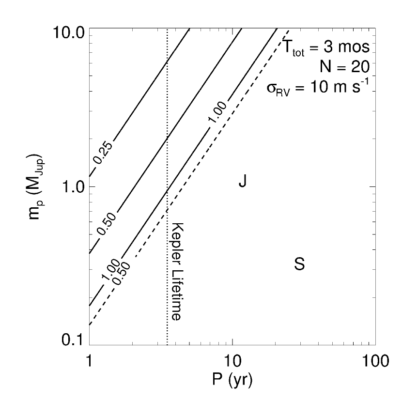
Contours of constant fractional uncertainty in the mass of the planet are shown in Fig. 8 as a function of $P$ and $m_{\rm p}$, assuming $N=20$ radial velocity measurements are taken over $T_{\rm tot}=3$ mos with a precision $\sigma_{\rm RV}=10{\rm\,m\,s}^{-1}$. It shows that the planet mass can be estimated to within a factor of two over this time period, thus establishing the planetary nature of the transiting object. By doubling the length of observations, one can put stronger constraints on the mass of the planet.

There are two points to bear in mind when applying this estimate for the uncertainty in the mass of the planet. First, for $r_{\rm p}\lesssim R_{\rm Neptune}$, the $Q^{-2}(24T/\tau)$ term is no longer small. The second consideration is that as time progresses away from the time of transit, the straight line approximation to the radial velocity curve will break down. In that case, the period will begin to be constrained by the radial velocity curve itself, and the uncertainties should be calculated from a Fisher matrix analysis of the full expression for the radial velocity curve with three parameters: $v_{0}$, $K_{\star}$, and $P$.

Figure 8: Contours of constant uncertainty in $m_{\rm p}$ as a function of $m_{\rm p}$ and $P$. The solid lines show the result for 20 radial velocity measurements with precision of $10~{}{\rm m~{}s^{-1}}$ taken over a period of 3 months after the transit. The dashed line shows the contour for $\sigma_{m_{\rm p}}/m_{\rm p}=0.50$ for 40 observations taken over 6 months. The dotted line indicates the mission lifetime of 3.5 years. The positions of Jupiter and Saturn are indicated.

6 Eccentricity

The results presented in the previous sections assumed circular orbits. Given that the average eccentricity $e$ of planets with $P\geq 1~{}{\rm yr}$ is $e\simeq 0.3$, this is not necessarily a good assumption. In this section, we assess the effects of non-zero eccentricities on the ability to characterize single-transit events detected by Kepler. We note that our discussion has some commonality with the study of Ford et al. (2008), who discuss the possibility of characterizing the orbital eccentricities of transiting planets with photometric observations. However, our study addresses this topic from a very different perspective.

In §3 we demonstrated that, under the assumption that $e=0$, the planet period $P$ and mass $m_{\rm p}$ can be inferred from two observables: the velocity of the planet at the time of transit $v_{\rm tr}$, and the projected acceleration of the star $A_{\star}$. In the case of a non-zero eccentricity, there are two additional unknown parameters: the eccentricity $e$ and the argument of periastron of the planet $\omega_{p}$. Thus, with only two observables ($v_{\rm tr}$ and $A_{\star}$) and four unknowns ($P,m_{\rm p},e,\omega_{p}$), it is not possible to obtain a unique solution.

Although a unique solution to the planet parameters does not exist using the observable parameters alone, it may nevertheless be possible to obtain an interesting constraint on $P$ and/or $m_{\rm p}$ by adopting reasonable priors on $e$ and $\omega_{p}$. From the transit observables, one can estimate the velocity of the planet at the time of transit (Eq. 6). In the case of $e\neq 0$, this is given by,

$$v_{\rm tr,p}=\frac{2\pi a}{P}\frac{1+e\sin\omega_{p}}{(1-e^{2})^{1/2}},$$ (33)

where here and throughout this section we assume $\sin i=1$. Solving for $P$,

$$P=\frac{2\pi GM_{\star}}{v_{\rm tr,p}^{3}}\left[\frac{1+e\sin\omega_{p}}{(1-e^{2})^{1/2}}\right]^{3}.$$ (34)

For a fixed value of $e$, the inferred period relative to the assumption of a circular orbit has extremes due to the unknown value of $\omega_{p}$ of

$$\left(\frac{\Delta P}{P}\right)_{min/max}=\left(\frac{1+e}{1-e}\right)^{\pm 3/2}.$$ (35)

Taking a typical value for the eccentricity of $e=0.3$, this gives a range of inferred periods of $0.4-2.5$ relative to the assumption of a circular orbit. In fact, because the probability that a planet with a given $a$ transits its parent star depends on $e$ and $\omega_{p}$ (Barnes, 2007; Burke, 2008), a proper Bayesian estimate, accounting for these selection effects, might reduce the range of inferred values for $P$ significantly.

What can be learned from RV observations immediately after the transit? Expanding the stellar projected velocity around the time of transit, we can write,

$$v_{\star}=v_{0}+eK_{*}\cos{\omega_{p}}-A_{\star}(t-t_{c})+\frac{1}{2}J_{\star}(t-t_{c})^{2}.$$ (36)

The projected acceleration of the star at the time of transit is,

$$A_{\star}=\frac{Gm_{\rm p}}{a^{2}}\left(\frac{1+e\sin\omega_{p}}{1-e^{2}}\right)^{2}.$$ (37)

This can be combined with $v_{\rm tr,p}$ to derive the mass of the planet,

$$m_{\rm p}=\frac{GM_{\star}^{2}}{v_{\rm tr,p}^{4}}A_{\star}(1+e\sin\omega_{p})^{2}$$ (38)

Thus, for a fixed eccentricity, the inferred mass relative to the assumption of a circular orbit has extremes of,

$$\left(\frac{\Delta m_{\rm p}}{m_{\rm p}}\right)_{min/max}=(1\pm e)^{2},$$ (39)

which for $e=0.3$ yields a range of $0.5-1.7$, which is generally smaller than the contribution to the uncertainty in $m_{\rm p}$ due to the measurement uncertainty in $A_{\star}$ for our fiducial case of $m_{\rm p}=M_{\rm Jup}$ and $P=3.5~{}{\rm yrs}$ (see Eq. 18) .

We may also consider what can be learned if it is possible measure the curvature of the stellar radial velocity variations immediately after transit. The projected stellar jerk is given by,

$$J_{\star}=\frac{4\pi Gm_{\rm p}}{Pa^{2}}\frac{(1+e\sin\omega_{p})^{3}e\cos\omega_{p}}{(1-e^{2})^{7/2}}.$$ (40)

This can be combined with $v_{\rm tr}$ and $A_{\star}$ to provide an independent constraint on a combination of the eccentricity and argument of periastron,

$$\frac{e\cos\omega_{p}}{(1+e\sin\omega_{p})^{2}}=\frac{GM_{\star}J_{\star}}{2A_{\star}v_{\rm tr}^{3}}.$$ (41)

Unfortunately, it will be quite difficult to measure $J_{\star}$. Using the same Fisher formalism as we used to estimate the uncertainty in $A_{\star}$ (§8), assuming $N$ evenly-spaced RV measurements with precision $\sigma_{\rm RV}$, taken over time span $T_{\rm tot}$ after the transit, the uncertainty in $J_{\star}$ is,

$$\sigma_{J_{\star}}^{2}\simeq\frac{720\sigma_{\rm RV}^{2}}{NT_{\rm tot}^{4}},$$ (42)

where we have assumed $N\gg 1$. For our fiducial parameters, the fractional uncertainty in $J_{\star}$ is,

$$\left(\frac{\sigma_{J_{\star}}}{J_{\star}}\right)^{2}\simeq 710\left(\frac{\sigma_{\rm RV}}{10{\rm\,m\,s}^{-1}}\right)^{2}\left(\frac{3{\rm\,mos}}{T_{\rm tot}}\right)^{4}\left(\frac{20}{N}\right)\left(\frac{M_{\rm Jup}}{m_{\rm p}}\right)^{2}\left(\frac{M_{\star}}{M_{\odot}}\right)^{4/3}\left(\frac{P}{3.5{\rm\,yrs}}\right)^{10/3}\left(\frac{e\cos{\omega_{p}}}{0.3}\right)^{-2},$$ (43)

where we have approximated $e\cos{\omega_{p}}(1+e\sin{\omega_{p}})^{3}(1-e^{2})^{-7/2}\sim e\cos{\omega_{p}}$. We conclude that, in order to obtain interesting constraints on the eccentricity of long-period planets detected by Kepler, higher-precision RV measurements taken over a baseline comparable to $\sim P$ will be needed.

7 Summary

The discovery of long-period transiting planets along with subsequent follow-up observations would greatly enhance our understanding of the physics of planetary atmospheres and interiors. Such planets would allow us to gather constraints in a regime of parameter space currently only occupied by our own giant planets, namely planets whose energy budgets are dominated by their residual internal heat, rather than by stellar insolation. These constraints, in turn, might provide new insights into planet formation. In this paper, we demonstrated that it will be possible to detect and characterize such long-period planets using observations of single transits by the Kepler satellite, combined with precise radial velocity measurements taken immediately after the transit. Indeed, these results can be generalized to any transiting planet survey using the scaling relations we provide, and it may be particularly interesting to apply them to the COnvection, ROtation & planetary Transits (CoRoT) mission (Baglin, 2003).

We calculated that Kepler will see a few long-period, single transit events and showed that, for circular orbits, the period of the system can be derived from the Kepler light curve of a single event. We derived an expression for the uncertainty in this period and showed that it is dominated by the uncertainty in the stellar density derived from spectroscopy (which we assume is $\sim 10\%$) for planets with radii larger than the radius of Neptune, rather than being dependent on the properties of the transit itself. This method can also be applied to planets that Kepler will observe more than once, so that the second time a planet is expected to transit Kepler can make a selective improvement to its time sampling to better characterize the transit.

We have also shown how the mass of the planet can be constrained by acquiring precise ($\sim 10~{}{\rm m~{}s^{-1}}$) radial velocity measurements beginning shortly after the transit occurs. We have shown that 20 measurements over 3 months can measure the mass of a Jupiter-sized object to within a factor of a few and that extending those observations to 40 measurements over 6 months significantly reduces the uncertainty in the mass. Knowing the mass to within a factor of a few in such a short time can distinguish between brown dwarfs and planets rapidly and allow us to maximize our use of radial velocity resources.

We explored the effect of eccentricity on the ability to estimate the planet mass and period. Allowing for a non-zero eccentricity adds two additional parameters, and as a result it is not possible to obtain a unique solution for the planet mass, period, eccentricity, and argument of periastron. However, by adopting a reasonable prior on the eccentricity of the planet, the period and mass of the planet can still be estimated to within a factor of a few. Detailed characterization of the planet properties will require precision RV measurements obtained over a duration comparable to the period of the planet.

Thus, in the interest of “getting the most for your money,” we have shown that the sensitivity of Kepler extends to planets with periods beyond its nominal mission lifetime. With the launch of the Kepler satellite, we are poised to discover and characterize several long-period transiting systems, provided that we are prepared to look for them.

8 Appendix: Detailed Derivations

8.1 Derivation of the Uncertainties in the Light Curve Observables

The Fisher matrix formalism is a simple way to estimate the uncertainties in the parameters, $\alpha$, of a model $F(x)$, that is being fit to a series of measurements $x_{k}$ with measurement uncertainties $\sigma_{k}$. The covariance of $\alpha_{i}$ with $\alpha_{j}$ is given by the element $c_{ij}$ of the covariance matrix $c$, where $c=b^{-1}$ and the entries of $b$ are given by,

$$b_{ij}\equiv\displaystyle\sum_{k=1}^{N_{d}}\frac{\partial F(x_{k})}{\partial\alpha_{i}}\frac{\partial F(x_{k})}{\partial\alpha_{j}}\frac{1}{\sigma_{k}^{2}},$$ (44)

where $N_{d}$ is the number of data points. In the limit of infinite sampling ($N_{d}\rightarrow\infty$) and fixed precision, $\sigma_{k}=\sigma$,

$$b_{ij}\rightarrow\frac{1}{D\sigma^{2}}\displaystyle\int_{0}^{D}\frac{\partial F(x)}{\partial\alpha_{i}}\frac{\partial F(x)}{\partial\alpha_{j}}\,dx,$$ (45)

where the interval of interest is given by $x=[0,D]$, and in this case $D$ is the total duration of observations. Thus, if the partial derivatives of a model with respect to its parameters are known, then the uncertainties in those parameters can be estimated (Gould, 2003).

For the simplified transit model described in $\S$4.1, the observable parameters are $\alpha=[t_{c},T,\tau,\delta,F_{0}]$. For a sampling rate $\gamma$, the $b$ matrix is,

$$b=\frac{\gamma}{\sigma^{2}}\left(\begin{array}[]{ccccc}\frac{2\delta^{2}}{\tau}&0&0&0&0\\ 0&\frac{\delta^{2}}{2\tau}&0&\frac{\delta}{2}&-\delta\\ 0&0&\frac{\delta^{2}}{6\tau}&-\frac{\delta}{6}&0\\ 0&\frac{\delta}{2}&-\frac{\delta}{6}&T-\frac{\tau}{3}&-T\\ 0&-\delta&0&-T&D\end{array}\right).$$ (46)

The covariance matrix is,

$$c=b^{-1}=\left(\frac{\sigma^{2}}{\gamma T\delta^{2}}\right)\left(\begin{array}[]{ccccc}\frac{\tau T}{2}&0&0&0&0\\ 0&-\frac{\tau T(D\tau-2DT+2T^{2})}{t_{out}t_{f}}&-\frac{\tau^{2}T(D-2T)}{t_{out}t_{f}}&-\frac{\tau T\delta(D-2T)}{t_{out}t_{f}}&\frac{\tau T\delta}{t_{out}}\\ 0&-\frac{\tau^{2}T(D-2T)}{t_{out}t_{f}}&-\frac{\tau T(5D\tau-4\tau^{2}-6DT+6T^{2})}{t_{out}t_{f}}&\frac{\tau T\delta(D-2\tau)}{t_{out}t_{f}}&\frac{\tau T\delta}{t_{out}}\\ 0&-\frac{\tau T\delta(D-2T)}{t_{out}t_{f}}&\frac{\tau T\delta(D-2\tau)}{t_{out}t_{f}}&\frac{T\delta^{2}(D-2\tau)}{t_{out}t_{f}}&\frac{T\delta^{2}}{t_{out}}\\ 0&\frac{\tau T\delta}{t_{out}}&\frac{\tau T\delta}{t_{out}}&\frac{T\delta^{2}}{t_{out}}&\frac{T\delta^{2}}{t_{out}}\end{array}\right),$$ (47)

where $t_{f}\equiv T-\tau$ is the duration of the flat part of the eclipse and $t_{out}\equiv D-\tau-T$ is the time spent out of eclipse. Thus, the uncertainty on the ingress/egress time, $\sigma_{\tau}$, is given by

$$\sigma_{\tau}=\sqrt{c_{33}}=\frac{\sigma}{\sqrt{\gamma}}\sqrt{\frac{-\tau(5D\tau-4\tau^{2}-6DT+6T^{2})}{\delta^{2}t_{out}t_{f}}}.$$ (48)

Define $Q\equiv\sqrt{\gamma T}(\delta/\sigma)$. Then, in the limit $\tau\ll T$, the uncertainties in the observable parameters are given by,

$$\sigma_{t_{c}} =Q^{-1}\sqrt{\frac{T\tau}{2}}$$ (49)

$$\frac{\sigma_{T}}{T} =Q^{-1}\sqrt{\frac{2\tau}{T}}$$ (50)

$$\frac{\sigma_{\tau}}{\tau} =Q^{-1}\sqrt{\frac{6T}{\tau}}$$ (51)

$$\frac{\sigma_{\delta}}{\delta} =Q^{-1}\sqrt{\frac{1}{\left(1-\frac{T}{D}\right)}}$$ (52)

$$\frac{\sigma_{F_{0}}}{F_{0}} =0\mbox{ , since in general, $\delta\ll F_{0}$}.$$ (53)

Note that $Q$ is approximately the total signal-to-noise ratio of the transit. Assuming that the photometric uncertainties are limited by photon noise, we have that $\gamma/\sigma^{2}=\Gamma_{\rm ph}$, where $\Gamma_{\rm ph}$ is the photon collection rate. This recovers the expression for $Q$ in §3.

A more detailed analysis of the variances and covariances of the transit observables can be found in Carter et al. (2008).

8.2 Derivation of the Uncertainties from the Radial Velocity Curve

A similar analysis can be done for the radial velocity curve, except that we use Eq. 44 and consider discrete observations. The radial velocity for a circular orbit is

$$v_{\star}=v_{0}-K_{\star}\sin\left[\frac{2\pi}{P}(t-t_{c})\right]$$ (54)

Expanding about $t_{c}$ gives

$$v_{\star}=v_{0}-K_{\star}\frac{2\pi}{P}(t-t_{c})=v_{0}-A_{\star}(t-t_{c}),$$ (55)

where $A_{\star}$ is the stellar projected acceleration at the time of the transit,

$$A_{\star}=\frac{2\pi K_{\star}}{P}.$$ (56)

Consider $N$ measurements of $v_{\star}$, each with precision $\sigma_{\rm RV}$, taken at times $t_{k}$. Fitting these measurements to the linear model in Eq. 55, we can estimate the uncertainties in the parameters $v_{0}$ and $A_{\star}$ using the Fisher matrix formalism,

$$b=\frac{1}{\sigma^{2}}\left[\begin{array}[]{cc}N&-\displaystyle\sum_{k=1}^{N}(t_{k}-t_{c})\\ -\displaystyle\sum_{k=1}^{N}(t_{k}-t_{c})&\displaystyle\sum_{k=1}^{N}(t_{k}-t_{c})^{2}\end{array}\right].$$ (57)

The covariance matrix is the inverse of $b$,

$$c=\frac{\sigma^{2}}{\left[\displaystyle\sum_{k=1}^{N}(t_{k}-t_{c})^{2}\right]-\left[\displaystyle\sum_{k=1}^{N}(t_{k}-t_{c})\right]^{2}}\left[\begin{array}[]{cc}\displaystyle\sum_{k=1}^{N}(t_{k}-t_{c})^{2}&\displaystyle\sum_{k=1}^{N}(t_{k}-t_{c})\\ \displaystyle\sum_{k=1}^{N}(t_{k}-t_{c})&N\end{array}\right].$$ (58)

If the points are evenly spaced by $\Delta t$

$$\displaystyle\sum_{k=1}^{N}(t_{k}-t_{c})=\displaystyle\sum_{k=1}^{N}k\Delta t=\frac{N(N+1)}{2}\Delta t,$$ (59)

$$\displaystyle\sum_{k=1}^{N}(t_{k}-t_{c})^{2}=\displaystyle\sum_{k=1}^{N}(k\Delta t)^{2}=\frac{N(N+1)(2N+1)}{6}\Delta t^{2},$$ (60)

and thus,

$$c = \frac{\sigma^{2}}{N(N-1)\Delta t^{2}}\left[\begin{array}[]{cc}2(2N+1)\Delta t^{2}&6\Delta t\\ 6\Delta t&\frac{12}{(N+1)}\end{array}\right].$$ (63)

The uncertainty in the projected stellar acceleration is,

$$\sigma_{A_{\star}}^{2}=\frac{\sigma_{\rm RV}^{2}}{N(N-1)(N+1)(\Delta t)^{2}}.$$ (64)

In the limit as $N\rightarrow\infty$, the covariance matrix reduces to,

$$c = \frac{\sigma_{\rm RV}^{2}}{\Delta t^{2}}\left[\begin{array}[]{cc}\frac{4\Delta t^{2}}{N}&\frac{6\Delta t}{N^{2}}\\ \frac{6\Delta t}{N^{2}}&\frac{12}{N^{3}}\end{array}\right].$$ (67)

Defining the total length of observations as $T_{\rm tot}\equiv N\Delta t$, we can also write,

$$c = \frac{\sigma_{\rm RV}^{2}}{T_{\rm tot}^{2}}\left[\begin{array}[]{cc}4\frac{T_{\rm tot}}{N}&6\frac{T_{\rm tot}}{N}\\ 6\frac{T_{\rm tot}}{N}&\frac{12}{N}\end{array}\right],$$ (70)

and so the uncertainty $A_{\star}$ in the limit of $N\rightarrow\infty$ becomes,

$$\sigma_{A_{\star}}^{2}=\frac{12\sigma_{\rm RV}^{2}}{T_{\rm tot}^{2}N}.$$ (71)

References

- Baglin (2003) Baglin, A. 2003, Advances in Space Research, 31, 345
- Barnes (2007) Barnes, J. W. 2007, PASP, 119, 986
- Basri et al. (2005) Basri, G., Borucki, W. J., & Koch, D. 2005, New Astronomy Review, 49, 478
- Beaulieu et al. (2006) Beaulieu, J.-P., Bennett, D. P., Fouqué, P., Williams, A., Dominik, M., Jørgensen, U. G., Kubas, D., Cassan, A., Coutures, C., Greenhill, J., Hill, K., Menzies, J., Sackett, P. D., Albrow, M., Brillant, S., Caldwell, J. A. R., Calitz, J. J., Cook, K. H., Corrales, E., Desort, M., Dieters, S., Dominis, D., Donatowicz, J., Hoffman, M., Kane, S., Marquette, J.-B., Martin, R., Meintjes, P., Pollard, K., Sahu, K., Vinter, C., Wambsganss, J., Woller, K., Horne, K., Steele, I., Bramich, D. M., Burgdorf, M., Snodgrass, C., Bode, M., Udalski, A., Szymański, M. K., Kubiak, M., Wiȩckowski, T., Pietrzyński, G., Soszyński, I., Szewczyk, O., Wyrzykowski, Ł., Paczyński, B., Abe, F., Bond, I. A., Britton, T. R., Gilmore, A. C., Hearnshaw, J. B., Itow, Y., Kamiya, K., Kilmartin, P. M., Korpela, A. V., Masuda, K., Matsubara, Y., Motomura, M., Muraki, Y., Nakamura, S., Okada, C., Ohnishi, K., Rattenbury, N. J., Sako, T., Sato, S., Sasaki, M., Sekiguchi, T., Sullivan, D. J., Tristram, P. J., Yock, P. C. M., & Yoshioka, T. 2006, Nature, 439, 437
- Borucki et al. (2004) Borucki, W., Koch, D., Boss, A., Dunham, E., Dupree, A., Geary, J., Gilliland, R., Howell, S., Jenkins, J., Kondo, Y., Latham, D., Lissauer, J., & Reitsema, H. 2004, in ESA Special Publication, Vol. 538, Stellar Structure and Habitable Planet Finding, ed. F. Favata, S. Aigrain, & A. Wilson, 177–182
- Burke (2008) Burke, C. J. 2008, arXiv:0801.2579, 801
- Butler et al. (2006) Butler, R. P., Wright, J. T., Marcy, G. W., Fischer, D. A., Vogt, S. S., Tinney, C. G., Jones, H. R. A., Carter, B. D., Johnson, J. A., McCarthy, C., & Penny, A. J. 2006, ApJ, 646, 505
- Carter et al. (2008) Carter, J. A., Yee, J. C., Eastman, J., Gaudi, B. S., & Winn, J. N. 2008, arXiv:0805.0238, 805
- Charbonneau et al. (2005) Charbonneau, D., Allen, L. E., Megeath, S. T., Torres, G., Alonso, R., Brown, T. M., Gilliland, R. L., Latham, D. W., Mandushev, G., O’Donovan, F. T., & Sozzetti, A. 2005, ApJ, 626, 523
- Charbonneau et al. (2002) Charbonneau, D., Brown, T. M., Noyes, R. W., & Gilliland, R. L. 2002, ApJ, 568, 377
- Claret (2000) Claret, A. 2000, A&A, 363, 1081
- Cumming et al. (2008) Cumming, A., Butler, R. P., Marcy, G. W., Vogt, S. S., Wright, J. T., & Fischer, D. A. 2008, arXiv:0803.3357, 803
- Deming et al. (2005) Deming, D., Seager, S., Richardson, L. J., & Harrington, J. 2005, Nature, 434, 740
- Ford et al. (2008) Ford, E. B., Quinn, S. N., & Veras, D. 2008, arXiv:0801.2591, 801
- Gould (2003) Gould, A. 2003, arXiv:astro-ph/0310577
- Gould et al. (2006) Gould, A., Udalski, A., An, D., Bennett, D. P., Zhou, A.-Y., Dong, S., Rattenbury, N. J., Gaudi, B. S., Yock, P. C. M., Bond, I. A., Christie, G. W., Horne, K., Anderson, J., Stanek, K. Z., DePoy, D. L., Han, C., McCormick, J., Park, B.-G., Pogge, R. W., Poindexter, S. D., Soszyński, I., Szymański, M. K., Kubiak, M., Pietrzyński, G., Szewczyk, O., Wyrzykowski, Ł., Ulaczyk, K., Paczyński, B., Bramich, D. M., Snodgrass, C., Steele, I. A., Burgdorf, M. J., Bode, M. F., Botzler, C. S., Mao, S., & Swaving, S. C. 2006, ApJ, 644, L37
- Mandel & Agol (2002) Mandel, K. & Agol, E. 2002, ApJ, 580, L171
- Rowe et al. (2007) Rowe, J. F., Matthews, J. M., Seager, S., Miller-Ricci, E., Sasselov, D., Kuschnig, R., Guenther, D. B., Moffat, A. F. J., Rucinski, S. M., Walker, G. A. H., & Weiss, W. W. 2007, arXiv:0711.4111, 711
- Seager & Mallén-Ornelas (2003) Seager, S. & Mallén-Ornelas, G. 2003, ApJ, 585, 1038