Tracing the equation of state and the density of cosmological constant along z
Abstract
We investigate the equation of state in a non–parametric form using the latest compilations of distance luminosity from SNe Ia at high z. We combine the inverse problem approach with a Monte Carlo to scan the space of priors. On the light of the latest high redshift supernova data sets, we reconstruct . A comparison between a sample including the latest results at z 1 and a sample without those results show the improvement achieved by observations of very high z supernovae. We present the prospects to measure the variation of dark energy density along z by this method.
Keywords: classical tests of cosmology – supernova type Ia
1 Introduction
The acceleration of the rate of expansion of the Universe, first discovered through supernovae [1, 2] is being examined through more extended samples of those distance indicators. In the next decade, large samples of supernovae and an increased coverage in z of the measurements of baryon acoustic oscillations (BAO) would allow to obtain the expansion rate and the equation of state [3, 4]. Complementary information on the matter density and global curvature provided by the CMB measurements from Planck [5] and weak lensing surveys [6] would enable to establish a better range of allowed regions in . SNe Ia together with BAO measurements up to very high z can be combined to restrict the range of possibilities of the empirical behavior of dark energy. By recovering the empirical behavior of one expects to test whether the acceleration of the expansion of the Universe indicates modifications of gravity beyond GR, whether it is due to the presence of vacuum energy or it is associated with a light scalar field ([7, 8, 9, 10, 11, 12, 13, 14, 15, 16]).
The recovery of the function from a given sample of data has been attempted proposing fitting functions or expansion series of along z in ways to accomodate a wide range of dark energy candidates. There has been some debate on the effect that choosing particular models for those functions or truncating the expansion series in z might have in deriving possible evolution [17, 18, 19].
Here, we use an approach to obtain without imposing any constraints on the form of the function. This is obtained through a generalized nonlinear inverse approach. The inverse approach formulated by Bakus and Gilbert [20] has been widely used in geophysics and solar structure physics. In this approach, the mere fact that the continuous functional has to be derived from a discrete number of data implies the non–uniqueness of the answer. It has also been shown that, even if the data were dense and with no uncertainty, there would be more than one solution to many specific inverse problems such as the determination of the density structure of the earth from the data on the local gravitational field at its surface, and others. This lack of uniqueness comes from the way in which the different equations reflect in the observables used. The problem of the determination of dark energy faces such degeneracy. In the luminosity distance along z from supernovae and other cosmic distance indicators, enters in an integral form, which limits the possibility to access to . In earlier examinations of the degeneracy in obtained through cosmic distance indicators, a range of solutions giving the same luminosity distance along z were pointed out [21]. As more data would constrain at various redshifts the reconstruction should become more successful. Here, we examine this using the latest compilations by Wood–Vasey et al (2007) [22] and Davis al (2007) [23] which use supernovae gathered by many collaborations and add new ones from ESSENCE, SNLS and the Higher–Z Team.
To compare with a significant body of work which analyses the data using the expansion to first order [24, 25], we will also formulate this approach for the case of determination of discrete parameters. We examine from current data the possibility of determining at present the values of and its first derivative and compare with previous results. It is known (see for instance [18]) that this approximation does not allow to recover properly the value of at high z. And it has been argued [19] that this expansion might bias towards faster evolution. It is, however, a very useful approach to restrict quintessence proposals. Given its widespread use, we include here the discrete case with the two parameters and .
In the following section, we introduce the inverse approach and deduce the equations for both the continuous and the discrete case. Then, we show the reconstruction of with current SNeIa data. Finally, we draw our conclusions.
2 Inverse problem
2.1 Non–parametric non–linear inversion
The inverse problem provides a powerful way to determine the values of functional forms from a set of observables. This approach is useful when the information along a certain coordinate, in our case information on , emerges in observables coupled with information at all other z as it happens with the luminosity distance. Dark energy is here addressed using the non–linear non–parametric inversion. Most frequently, when the parameters to be determined are a set of discrete unknowns, the method used is a least squares. But the continuous case, where functional forms are to be determined, requires a general inverse problem formulation. The inverse method used here is a Bayesian approach to this generalization [26].
We consider a flat universe with only two dominant constituents (at present): cold matter and dark energy. Therefore we characterize the cosmological model by the density of matter, , and by the index of the dark energy equation of state,
| (1) |
The vector of unknowns M has then a discrete and a continuous component,
| (2) |
On the other hand, the observational data are SNe Ia magnitudes. We have a finite set of magnitudes, , and consider the following theoretical equation, the magnitude-redshift relation in a flat universe relating the unknowns to the observational data:
| (3) |
where is the Hubble-free luminosity distance
| (4) |
with
| (5) |
| (6) |
We redefine our data and convert the original SNe magnitudes to dimensionless distance coordinates :
| (7) |
| (8) |
where is the distance modulus. With this definition, we deal directly with a function , the only part which depends on the cosmological model.
After the corresponding transformations, the observables are now described by a vector of components, , and by a covariance matrix, . This method can handle correlated measurements, where non–diagonal elements are different from zero (observations i and j being correlated). But, at present, those have not been estimated for the composite samples of distance indicators. We would then use:
| (9) |
Similarly, the unknown vector of parameters is described by its a priori value, , and the covariance matrix, . The function describing is expected to be smooth, and this leads to no null covariance between neighboring points in z for . Thus, the covariance matrix has the form:
| (10) |
where a choice is made for the non–null covariance between z and z′, . This choice is taken to be as general as possible. It would define the smoothness required in the solution by setting the correlation length between errors in z and z′ (this gives the length scale in which the function can fluctuate between redshifts). The amplitude of the fluctuation of the function is given by the dispersion at z.
Thus for a Gaussian choice, is described as:
| (11) |
which means that the variance at z equals and that the correlation length between errors is . Another possible choice for is an exponential of the type:
| (12) |
while no difference in the results is found by those different choices.
This is all the information we have beforehand, and with that we are interested in determining the best estimator for M. The probabilistic approach we will use incorporates constraints from priors through the Bayes theorem, i.e, the a posterori probability density for the vector M containing the unknown model parameters given the observed data D, is linked to the likelihood function L and the prior density function for the parameter vector as:
| (13) |
The theoretical model described by the operator , which connects the model parameters M with the predicted data , is to agree as closely as possible with the observed data y. Assuming that both the prior probability and the errors in the data are distributed as Gaussian functions, the posterior distribution becomes:
| (14) |
where ∗ stands for the adjoint operator. The best estimator for M, , is the most probable value of M, given the set of data y. The condition is reached by minimizing the misfit function:
| (15) |
which is equivalent to maximize the Gaussian density of probability when data and parameters are treated in the same way. This Bayesian approach helps to regularize the inversion.
Let us now define the operator G represented by the matrix of partial derivatives of the dimensionless distance coordinate, which will simplify subsequent notation. Its kernel will be denoted by as defined in the next equations.
| (16) |
with
| (17) |
| (18) |
As shown in Eq. 3 or equivalently Eq. 7, the inverse problem is nonlinear in the parameters, thus the solution is reached iteratively in a gradient based search. To minimize in Eq. 15, one demands stationarity. For the nonlinear case the solution has to be implemented as an iterative procedure where [26]:
| (19) |
Since we are working in a Hilbert space with vectors containing functional forms, the above operator products give rise to scalar products of the functions integrated over the domain of those functions. The expressions transform into having the products rewritten in terms of the kernels of the operators [27].
We will indicate the scalar product by “ ” and it is defined as it can be seen from this example:
| (20) |
The components of the vector of unknowns , which in our case will be both and , are then obtained from:
| (21) |
where
| (22) |
| V | |||||
| (23) | |||||
| S | |||||
| (24) |
In the case of the dark energy equation of state and the matter density the expressions reduce to
| (25) |
| (26) |
where , is given by the product (22) with:
| (27) | |||||
| (28) |
To test the accuracy of the inversion we use the a posteriori covariance matrix. It can be shown (see [28, 27]) that for the linear inverse problem with Gaussian a priori probability density function, the a posteriori probability density function is also Gaussian with mean Eq. 2.1 and covariance Eq. 29. Although its value is only exact in the linear case it is a good approximation here, since the luminosity distance is quite linear on the equation of state at low redshift.
| (29) | |||||
In an explicit form, the standard deviations from this covariance read
| (30) |
| (31) |
where the symbols with tilde are the a posteriori values, whereas the symbols without represent the a priori ones. It must be stressed that the uncertainty in the final does depend on the a priori assumption of the uncertainty. In fact, the same could depend on the prior. For avoiding a dependence of the result and its error on the prior we use Monte Carlo methods later in the analysis.
There are other parameters which help to interpret the results. From the form of Eq. 29 we see that the operator is related to the obtained resolution. This is usually called the resolving kernel . The more this term resembles the -function the smaller the a posteriori covariance function is. In fact, in the linear case, the resolving kernel represents how much the results of the inversion differ from the true model. It equals to be the filter between the true model and its estimated value [20, 26]. In any applied case, it is a low band pass filter which depends on the data available and the details requested from the model. In a useful way, it can also be expressed in terms of the a priori and the a posteriori covariance matrices:
| (32) |
This expression will be evaluated numerically to quantify the resolution and information generated in the inversion.
2.2 Discrete parameters
In the previous section we have obtained the results for a set of a continuous function and a discrete parameter, but we can also consider the case of various discrete parameters. It was pointed out that a succesful parameterization for modeling a large variety of dark energy models is obtained by considering expanded around the scale factor . The earlier parameterization to first order in z given by proved unphysical for the CMB data and a poor approach to SN data at z 1. For the case of moderate evolution in the equation of state, the most simple (two–parameter) description of so far proposed is [25, 24]:
| (33) |
where the scale factor and turns out to be:
| (34) |
We use now this particular form for the function commonly used to study the behaviour of dark energy to solve iteratively for and :
| (35) |
| (36) |
where
| (37) |
| (38) |
The a posteriori variance is for these parameters:
| (39) |
| (40) |
3 Determination of
In the following, we determine using the inverse approach described above and the SNeIa by Davis et al. [23] which contains samples of high–z supernovae by various collaborations (the Supernova Cosmology Project, the High–Z Team, SNLS, the Higher–z team and ESSENCE).
Explicitly, one obtains the value of and at a given redshift with the equations of section 2.1 (Eqs. 25, 26, 30 and 31). In all the cases, it is assumed a flat universe, where the equations have been deduced, and a good knowledge for the density of matter: .
The a priori model as we will show is arbitrary for , but determines where the solution is searched. To avoid the possibility of having converged to a secondary minimum just because the prior is too far from the absolute one, we have also carried out a Monte Carlo (MC) exploration of the a priori model space. A flat distribution of 1000 models between has been randomly generated, and then the iterative process of inversion has been applied for all of them. We used for this inversion 1000 data sets obtained by bootstrap resampling of the original one. The MC exploration and the bootstrap approach allows to obtain the variance and deviation at every z in the non–parametric function . The resulting is obtained in this way.
Our results show with a Monte Carlo exploration with priors ranging from to that the obtained solution is stable.
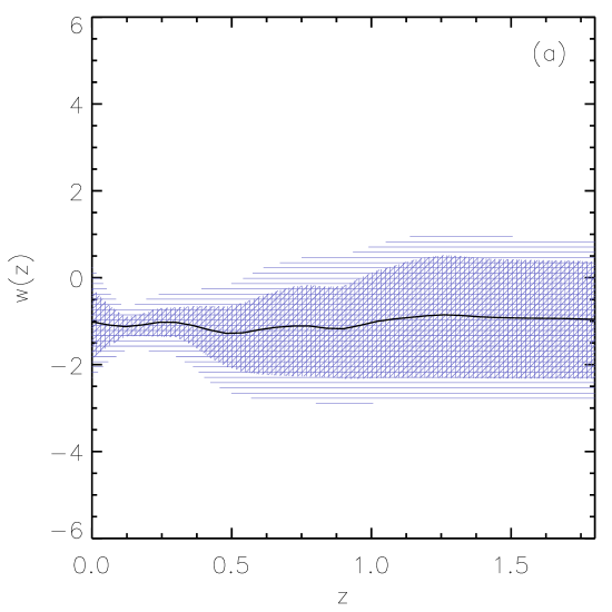
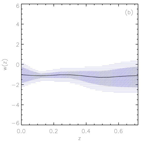
The solution using the 192 supernovae (60 from ESSENCE, 57 from SNLS and 45 nearby ones and 30 by Riess et al. 2006) is shown in Figure 1. The calculation uses redshift intervals of z 0.06. Various functional forms for the covariance have been tried giving the same results (covariance as in Eq. 12 or the Gaussian Eq. 11 give similar results). This calculation does not restrict fast evolving as the correlation length is kept to allow fast changes of slope (). In a situation where the data are scarce with very wide priors in the function , the solution can iterate between saddle points and local minima as few data do provide a landscape with no strong minima. However, in our case, the sample available for is large enough to allow to find the solution.
As it has been seen in Figure 1, at low and intermediate redshift the data delimit a narrow band of possible solutions. At low and intermediate redshift, where the inversion is reliable, there is no sign of any significant evolution. The cosmological constant is always within intervals.
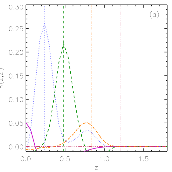
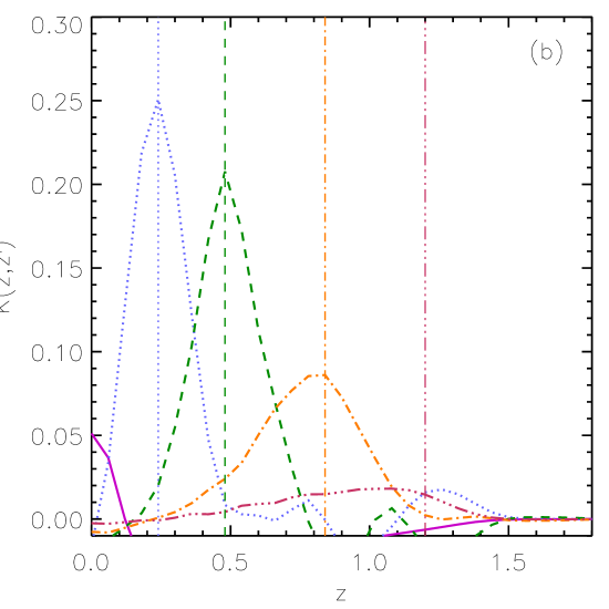
In Figure 1 the black solid line indicates the evolution of the equation of state, whereas the shadowed regions represents the 1 and 2 intervals. In Figure 2 the resolving kernels at z and are shown. It can be seen that only the prior is recovered at high redshift, where there is no information coming from data and the resolving kernels are almost flat. While Figure 1 show the results for the inversion using the [23] sample, very similar results are found if using the sample from [22]. The resolving kernels (Figure 2) indicate that the function is generally not well resolved at individual redshifts, well beyond the redshift range z . At high redshift, z for example, we observe a very wide and extremely flat , meaning that this redshift is not resolved at all by the data. The reliability of the inversion peaks in the range of z 0.2–0.5 where the information is maximum. This is also found in other analyses, though most of the reconstructions [31, 29, 19, 30] have been done prior to the availability of these combined samples.
Finally, one can particularize the continuos form of to a parameterization and compare the results with other analyses. Using the equations from Section 2.2 for , and with priors , and we obtained a positive evolution of the equation of state for the full data set: , (when excluding the highest z HST supernovae , ). This result agrees with the continuous evolutions seen before, as it is expected for a smooth and globally monotonous behaviour. For a constant equation of state, both data sets favour a cosmological constant within its intervals with a value of in the first case and in the second one.
4 A running cosmological constant as an inverse problem
We now use the power of the inverse method to detect an evolution of the cosmological constant. We interpret the unknown function as a running cosmological constant, but it can be interpreted as well as a general function of the dark energy density.
A running lambda can occur in various different scenarios (see for instance [11, 32] and references therein). We want to determine a general function such that
| (41) |
where is the value of for z 0. We use equations Eq. 4 and 5 to obtain the G matrix. We calculate the form of the best by computing in iterations until numerical convergence is obtained.
We tested various degrees of prior knowledge on . We display here the situation where we have a very precise knowledge of as it is expected after the Planck mission. If we knew well the matter density, we would see the evolution of , as in Figure 3.
The procedure for the inversion is the same as for the barotropic index of the equation of state. The uncertainty on the prior on is set to . The Monte Carlo exploration of the -space is made in the range . Since we are using the same data sets as in previous sections, we expect the same resolution. Therefore we use the same grid resolution.
For the two samples, VW07 and D07, the result of the inversion is quite similar. A constant density cannot be discarded. The reconstruction can not provide further information beyond redshift 0.6, but gives the behavior in the range 0 to 0.6. If we relax the prior knowledge of to a range of 0.03 we find a similar mean behavior but with a wider range of allowed values for . Figure 3 is shown for purposes of indicating the enormous value of the complementary information to be provided in the next future.
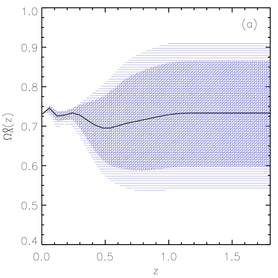
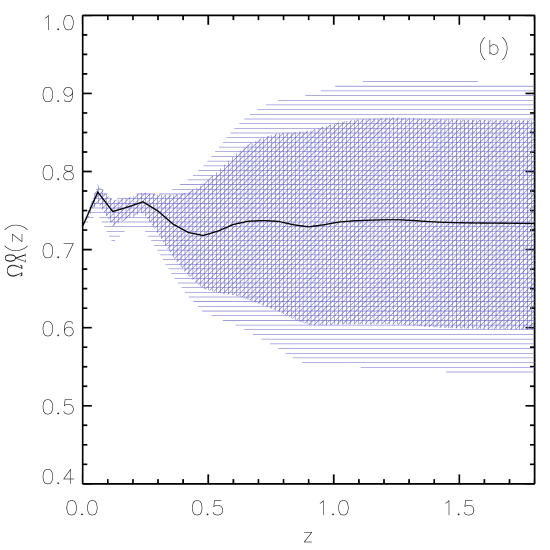
These reconstructions can be compared with the behavior of the cosmological constant in the running scenarios. Up to now, the obtained smooth evolutions down to redshifts lower than 1 are compatible with various scenarios for running cosmological constant as no fast changes are expected in the past Gyrs. Scenarios of moderate evolution with 0.1 [32] can be easily discarded with a good knowledge of .
5 Summary and conclusions
We introduce here an Inverse Problem approach to determine as a continuous function in a model–independent and non–parametric way. The resulting algorithm retrieves without imposing any constraints on the form of the function. The method uses Bayesian information such as the area where this solution is to be found, which can be quite unrestrictive. The approach explored here enables to see at which z is the maximum information on or in various samples.
The exploration of dark energy applying this method to the present SNe Ia sample helps to answer the question on whether there is evidence in the evolution of along z.
With the sets of 162 SNeIa and 192 SNe Ia [23, 22] we find compatible at 1 with a cosmological constant. The larger data set [23] shows improvement in the resolving kernels at high z. Error bars in both cases are big enough to make evident the limited knowledge that we have on . However, the bulk of data to come in the next decade and the complementary probes would allow to draw the behavior of and with much higher precision. This method can be applied to the determination of with both SNe Ia and BAO measurements.
References
References
- [1] Riess A G et al , 1998 Astron. J. 116 1009
- [2] Perlmutter S et al , 1999 Astrophys. J. 517 565
- [3] Bassett B A, Nichol B & Eisenstein D J 2005 Astronomy & Geophysics 46 526 [astro-ph/0510272]
- [4] Wang Y 2007 (Preprint 0710.3885)
- [5] http://www.rssd.esa.int/index.php?project=PLANCK
- [6] Heavens A F, Kitching T D & Taylor A N , 2006 Mon. Not. R. Astron. Soc. 373 105
- [7] Padmanabhan T 2003 Phys. Rep. 380 235
- [8] Sahni V and Starobinsky A 2006 Int. J. Mod. Phys. D 15, 2105
- [9] Copeland E J, Sami M & Tsujikawa S 2006 Int. J. Mod. Phys. D 15 1753
- [10] Ruiz–Lapuente P 2007 Class. Quantum Grav 24 R91
- [11] Nobbenhuis S 2006 Found. Phys. 36 631
- [12] Polarski D 2006 AIP Conf. Proc. 861 1013 [arXiv: astro-ph/0605532]
- [13] Stojkovic D, Starkman G D and Matsuo R 2008 Phys. Rev. D 77 063006 [arXiv: hep-ph/0703364)
- [14] Padmanabhan T 2008 Gen. Rel. Grav. 40 529 [arXiv:gr-qc/07052533]
- [15] Durrer R & Maartens R 2007 Gen. Rel. Grav 40 301 [arXiV 0711.0077]
- [16] Elizalde E, Jhingan S, Nojiri S, Odintsov S.D, Sami M & Thongkool I 2008 Eur. Phys. J. C53 447 [arXiv 0705.1211]
- [17] Bassett B A, Corasaniti P S & Kunz M, 2004 Astrophys. J. 617 L1 [astro-ph/0407364]
- [18] Bassett B A et al. 2007 [arXiv:0709.0526]
- [19] Riess A G et al , 2007 [astro-ph/0611572] Astrophysical Journal 656 98
- [20] Backus G and Gilbert F, 1970 Philos. Trans. R. Soc. London. Ser. A.366 123
- [21] Maor I, Brustein R & Steinhardt P J, 2001 Phys. Rev. Lett. 86 6
- [22] Wood-Vasey W M et al , 2007 Ap J 667, 694 [astro-ph/0701041]
- [23] Davis T M et al , 2007 Ap J 667, 716 [astro-ph/0701510]
- [24] Linder E V, 2003 Phys. Rev. Lett. 90, 091301
- [25] Chevallier M and Polarski D, 2001 Int. J. Mod. Phys. D 10 213 [gr-qc/0009008]
-
[26]
Tarantola A and Valette B, 1982 Rev. Geophys. & Space Phys. 20(2) 219
Tarantola A, Inverse Problem Theory, 1987 Elsevier, Amsterdam
http://www.ccr.jussieu.fr/tarantola/ - [27] Tarantola A and Nercessian A, 1984 Geophys. J. R. Astr. Soc. 76 299
- [28] Tarantola A and Valette B, 1982 J. Geophys. 50 159
- [29] Nesseris S and Perivolaropoulos L 2007 JCAP 0702 025 [astro-ph/0612653]
- [30] Perivolaropoulos L 2005 JCAP 0510 001
- [31] Zunckel C & Trotta R, 2007 Mon. Not. R. Astron. Soc. 380 865 [astro-ph/0702695]
- [32] España-Bonet C, Ruiz–Lapuente P, Shapiro I.L & Sola J 2004 JCAP 0402 006