INTEGRAL observations of the variability of OAO 1657$-$415

Abstract

Context. The Galactic Plane Scan (GPS) was one of the core observation programmes of the INTEGRAL satellite. The highly variable accreting pulsar OAO 1657$-$415 was frequently observed within the GPS.

Aims. We investigate the spectral and timing properties of OAO 1657$-$415 and their variability on short and long time scales in the energy range $6-160$ keV.

Methods. Using standard extraction tools and custom software for extracting INTEGRAL data we analysed energy-resolved light curves with a time resolution of one second – mainly data of the ISGRI instrument. We also analysed phase-averaged broad band spectra – including JEM-X spectra – and pulse-phase resolved spectra of ISGRI.

Results. During the time covered by the INTEGRAL observations, the pulse period evolution shows an initial spin-down, which is followed by an equally strong spin-up. In combining our results with historical pulse period measurements (correcting them for orbital variation) and with stretches of continuous observations by BATSE, we find that the long-term period evolution is characterised by a long-term spin-up overlayed by sets of relative spin-down/spin-up episodes, which appear to repeat quasi-periodically on a 4.8 yr time scale. We measure an updated local ephemeris and confirm the previously determined orbital period with an improved accuracy. The spectra clearly change with pulse phase. The spectrum measured during the main peak of the pulse profile is particularly hard. We do not find any evidence of a cyclotron line, wether in the phase-averaged spectrum or in phase-resolved spectra.

1 Introduction

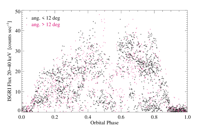
Figure 1: Orbital profile from 2687 individual science windows in the ISGRI energy range $20-40$ keV for source offset angles $<12\degr$ (black squares) and $12\degr-15\degr$ (red dots). Though the performance of the IBIS instrument significantly decreases for angles larger than $10\degr$, the count rate values for offset angles in the range $12\degr-15\degr$ are consistent with the count rates for angles below $12\degr$. The sharp decrease near phase 0.55 is clearly visible.

The accreting pulsar OAO 1657$-$415 was discovered by Polidan et al. (1978) with the Copernicus satellite. White & Pravdo (1979) detected a $38.22$ s pulsation, whereas the binary orbit and the eclipsing nature of the high mass binary system were discovered by Chakrabarty et al. (1993). The orbital period was later improved by Bildsten et al. (1997) from BATSE measurements to $P_{\mathrm{orb}}=(10\aas@@fstack{d}44809\pm 0\aas@@fstack{d}00030)$. As OAO 1657$-$415 lies in a heavily absorbed region, an optical counterpart could not be identified up to a limit of $V>23$, but an infrared counterpart was found by Chakrabarty et al. (2002). The infrared properties of OAO 1657$-$415 were found to be consistent with a highly reddened B supergiant. Analysing ASCA observations Audley et al. (2006) found a dust-scattered X-ray halo whose evidence decays through the eclipse. Using this halo they estimated a distance of $7.1\pm 1.3$ kpc. This is consistent with a source distance of $6.4\pm 1.5$ kpc derived by Chakrabarty et al. (2002) from photometric infrared measurements. The pulsar was found to show a long-term spin-up from $38.218$ s (White & Pravdo, 1979) to $37.329$ s (Chakrabarty et al., 2002) with intermediate spin-down periods (Bildsten et al., 1997) (see Table 2). This corresponds to an averaged long-time period derivative of $\dot{P}=-1.3\times 10^{-9}s\,s^{-1}$. For a time span of about 3300 days there are nearly continuous BATSE observations available with daily pulse period and flux values. Analysing the spin-up and spin-down episodes of BATSE data, Baykal (1997) found that the most natural explanation of X-ray flux and angular acceleration fluctuations is the formation of episodic accretion disks from stellar wind accretion. Lovelace et al. (1999) developed a model for magnetic, propeller driven outflows that cause a rapidly rotating magnetised star accreting from a disk to spin-down. Another model was introduced by Dai & Li (2006) in which they assume, in contrast to the model of Lovelace et al. (1999), that accretion continues during the (soft) propeller stage. This avoids otherwise occurring singularity problems and also leads to the fact that no significant changes in the X-ray luminosity occur during the spin transitions.

The spectral models commonly used for fitting the spectra of OAO 1657$-$415 usually include an absorbed power law model for the low energy part of the spectrum. For the high energy part an exponential cutoff power law model or a power law with high energy cutoff is used (see Sect. 4.1 for a definition of these models).

Orlandini et al. (1999) searched for cyclotron lines in BeppoSAX spectra of OAO 1657$-$415 and were able to fit a broad Lorentzian line at 30 keV with a width of 28 keV, using the exponential cutoff model for the continuum. As the width was quite large and not well constrained, they fixed the width at 10 keV, which changed the line position to 36 keV. Using the high energy cutoff continuum model, it was found that adding an absorption line did not significantly improve the fit. So Orlandini et al. (1999) concluded that the spectrum of OAO 1657$-$415 above 10 keV can be modelled by a series of three power laws with increasing steepness, such that no cyclotron line is needed.

Also, a fluorescence iron line emission was observed in this source with several instruments, e.g. ASCA (Audley et al., 2006), Chandra/HETGS (Chakrabarty et al., 2002), RXTE (Baykal, 2000), BeppoSAX (Orlandini et al., 1999) and Ginga (Kamata et al., 1990).

2 Observations and data reduction

The satellite INTEGRAL (Winkler et al., 2003a) is equipped with three instruments for the X- and $\gamma$-ray range: the spectrometer SPI (20 keV – 8 MeV) (Vedrenne et al., 2003), the imager IBIS (15 keV – 10 MeV) (Ubertini et al., 2003), and the X-ray monitor JEM-X ($3-60$ keV) (Lund et al., 2003). The imager IBIS consists of the low energy CdTe detector layer ISGRI ($15-1000$ keV) (Lebrun et al., 2003) and the high energy CsI detector layer PICsIT ($0.175-10.0$ MeV) (Labanti et al., 2003). IBIS has a fully coded field of view (FOV) of $9^{\circ}$ and a partially coded FOV of $19^{\circ}$ (50%). In this paper we have used ISGRI observations of OAO 1657$-$415, which were mainly part of the INTEGRAL Galactic Plane Scan (GPS). Being part of the core program of INTEGRAL, the GPS observations were performed as a sawtooth pattern along the accessible part of the Galactic plane with an extension in latitude of $\pm 10\degr$ (Winkler et al., 2003b). A total of 2687 science windows were available. One INTEGRAL science window (SCW) is a single observation of about 2000 s, so the total time of data acquisition was roughly $\sim 5$ Ms. The data used range from revolution 36 (MJD 52 668) up to revolution 463 (MJD 53 946).

Spectra were obtained also from JEM-X data. Due to a smaller FOV (fully coded $4\aas@@fstack{\circ}{}8$, partially (50%) coded $7\aas@@fstack{\circ}{}5$), only 41 science windows (SCWs) from JEM-X1 and 46 SCWs from JEM-X2 were available (selected from the SCWs used for ISGRI data, but with the angular distance of the centre of the FOV to the source restricted to $<4\aas@@fstack{\circ}{}5$). These were JEM-X2 observations of February and March 2003 and JEM-X1 observations from August 2004 to April 2005. As these 87 SCWs are just a small fraction of the total SCWs available from ISGRI observations, only phase-averaged spectra were produced (OSA 6.0), but no timing analysis was done for JEM-X data.

Generally, the observational data have been reduced using the Offline Scientific Analysis (OSA) software v. 6.0 provided by the INTEGRAL Science Data Centre, ISDC (Courvoisier et al., 2003). For generating spectra and pulse profiles from ISGRI data (spectral timing), an alternative software provided by the IASF Palermo (Ferrigno et al., 2007) was used.

For the timing analysis (including spectral timing analysis) we selected all observations for which OAO 1657$-$415 was within $12\degr$ from the centre of the FOV (this is recommended by ISDC since the reliability of the flux determination is reduced when the source is located in the outer parts of the partially coded FOV of ISGRI). For all existing science windows we determined the orbital phase and selected only data in the orbital phase interval from 0.1 to 0.9, thus excluding data during the eclipse.

Furthermore, we included only those science windows for which the count rate is above 15 s^-1 in the energy interval $20-40$ keV, corresponding to the “high state” (see below). The reason for this is that the timing analysis (the determination of the pulse period and in particular the determination of the pulse phase), needs data with a sufficient signal to noise ratio to yield significant results. All above mentioned restrictions left 842 science windows out of 2687 available (see also Fig. 1, which shows data from all available SCWs). Our results are therefore applicable to this “high state” only.

Figure 2: Averaged orbital profile in the ISGRI energy band $20-40$ keV. This profile was calculated from 1797 science windows for which the angular distance to the telescope axis was less than $12\degr$ (see text for description of error bars). The dashed line connects values giving the number of science windows (right axis) used for the respective averages.

3 Timing analysis

3.1 The orbital profile

Figure 1 shows the mean count rates from 2687 science windows in the ISGRI energy band $20-40$ keV as a function of orbital phase, which was calculated using the ephemeris of Bildsten et al. (1997) ($T_{90}$ = MJD 48 515.99 and $P_{\mathrm{orb}}$ = 10.448 09 d). The large scatter in this figure reflects the strong intrinsic variability of OAO 1657$-$415. Fig. 2 shows the averaged orbital profile, which was calculated from 1852 science windows (MJD $52\,668-53\,946$) for which the angular distance of OAO 1657$-$415 from the centre of the FOV was less than $12\degr$. The dashed line shows the number of science windows for each data point. In general, we confirm the asymmetric shape of the profile as it was measured by Wen et al. (2006) with ASM on board RXTE. In contrast to these measurements, the INTEGRAL observations show a remarkable minimum at phase 0.55, which is visible also in the ASM data averaged for the time range MJD $52\,668-53\,946$ (Fig. 3). The data presented by Wen et al. (2006) cover a time range of roughly 8.5 years ($\sim$ MJD $50\,160-53\,240$), which is much wider than the time range we analysed. We conclude therefore that the dip seen in our data might be a temporary phenomenon.

The lack of data points around $10-15$ counts s^-1 (cps) at orbital phases above 0.4 apparent in Fig. 1 may suggest the existence of a bimodal intensity distribution, defining a “high state” and a “low state” of this source.

The formal uncertainties of the count rates in Fig. 2 are negligible, but an unpredictable scatter is introduced by the fact that only in rare cases the continuous measurements span a complete orbit. Due to the intrinsic variability of the source the available data points do not represent a homogeneously averaged profile. The number of data points (Science Windows) per phase bin used to calculate the average flux varies between 40 and nearly 170. To evaluate the influence of the non-homogeneity of this sampling, we calculated profiles with a constant number of 30 SCWs per phase bin, randomly chosen from the available SCWs. We calculated 10 000 of these profiles and plotted the range between minimum and maximum values for each phase bin as “error bars” to Fig. 2. A discussion is given in Sect. 5.

Figure 3: Averaged orbital profile (ASM, $2-10$ keV) plotted from quick-look results provided by the ASM/RXTE team. This curve is calculated from 12830 single dwell values (sum band intensity) covering the used INTEGRAL observation period from MJD $52\,668-53\,946$. The error bars are quadrature averages of the flux errors. The dashed line shows the number of dwells per data point (right axis).

Figure 4: Determination of the centre of eclipse by fitting straight lines to ingress and egress. The dashed lines denote the width of the strips (0.03 phase units), which were used to determine the number of data points falling into the strips left and right to the fitted straight lines (see text). Only data points from SCWs with offset angles $<12\degr$ were used for this analysis (see Fig. 1).

Using the scatter plot shown in Fig. 1 we have determined the properties of the eclipse. The data points left and right of the apparent eclipse define a rather sharp boundary in phase space (orbital phase vs. count rate), leaving only a few individual outlying points. We fitted these boundaries by straight lines by maximising the differences in data points that fall into strips of predefined widths left and right to these lines (see Fig. 4). For ingress we fitted a line from 37 cps down to the maximum eclipse intensity of $\sim 3$ cps and the egress line from 3 cps to 20 cps. The strip widths were varied from 0.01 to 0.05 in phase units. No significant change of the fit parameters was observed for strip widths in the range $0.02-0.04$. We therefore used the average values obtained from the fits with 3 widths of 0.02, 0.03 and 0.04. The intersections of the ingress and egress lines with the bottom count rate are at orbital phases 0.899(5) and 1.052(5) (corresponding to MJD 52 662.84(5) and MJD 52 664.44(5), respectively), such that we set the centre of eclipse to phase 0.976(5) (MJD 52 663.64(5)), and the half width of the full eclipse to 0$\aas@@fstack{d}$80(3) (or $27\aas@@fstack{\circ}{}6\pm 1\aas@@fstack{\circ}{}0$). The MJD values are determined in such a way that they fall into the last orbit before our observations. The straight lines for ingress and egress are described by slopes (change of count rates) of 34 cps d^-1 and 28 cps d^-1, respectively, making the ingress faster than the egress by a factor of 1.2. We note that the above description gives upper limits to the speed of ingress or egress, individual events may be slower.

Table 1: Pulse periods of OAO 1657$-$415 as measured during the INTEGRAL GPS in 11 observation groups. The date is the centre of the observation time interval.

Grp.	Date	Range	Period	$\dot{P}$
	[MJD]	[d]	[s]	[$10^{-9}\leavevmode\nobreak\ s\,s^{-1}$]
1	52672.03	$\pm$0.67	37.1467 (1)
2	52711.48	$\pm$12.87	37.1645 (5)	$2.9\pm 1.0$
3	52859.94	$\pm$0.18	37.2028 (5)
4	52869.95	$\pm$0.91	37.2005 (5)
5	52908.42	$\pm$0.35	37.2008 (5)
6	53054.92	$\pm$0.07	37.2262 (50)
7	53232.53	$\pm$0.53	37.2712 (2)
8	53255.48	$\pm$0.36	37.2819 (3)
9	53464.74	$\pm$1.63	37.2060 (15)
10	53650.10	$\pm$0.57	37.1137 (7)
11	53789.58	$\pm$5.32	37.1209 (6)

3.2 Pulsar period analysis

The pulse period analysis was performed in steps, successively improving the accuracy of the analysis. This was necessary because of the strong variation in the pulse period over the time covered by the INTEGRAL GPS observations. We started out with an ISGRI light curve in the $20-200$ keV energy range with a time resolution of 1 s (produced by the IASF Palermo software${}^{\ref{fn_palermo}}$). The bin times were first converted to the solar system bary centre and then corrected for binary motion using the ephemeris of Bildsten et al. (1997) ($T_{90}$ = MJD 48 515.99(5), $P_{\mathrm{orb}}=10\aas@@fstack{d}448\,09(30)$, $a\sin i=106.0(5)$ lt-sec, $e=0.104(5)$ and $\omega=93(5)\degr$). For each SCW a period search with epoch folding was performed. This led to first estimates of the pulse periods and already clearly showed a strong variation with time. As a next step we produced pulse profiles combining four to five SCWs. A phase connection analysis of these profiles – by using the mean profile as a template and fitting the individual profiles to this template – (Deeter et al., 1981; Nagase, 1989; Muno et al., 2002) yielded significantly more accurate periods. A further refinement was reached using a smoothing technique: pulse profiles were generated (with the so far best pulse period) for data sets of at least eight SCWs, where the start of each data set was shifted by one SCW as compared to the start of the previous one. This produced “running mean pulse profiles” with good photon statistics, from which the final pulse periods were again determined by the phase connection technique (the loss of statistical independence between consecutive pulse profiles does not pose a problem here). The above described procedure was performed for each of the eleven groups of observations (the groups contained 12 to 273 SCWs). The final periods are listed in Table 1 and plotted in Fig. 5. Due to the short integration times it was generally not possible to measure a period derivative within one group of observations – except for group no. 2, for which we find a local $\dot{P}$ of $(2.9\pm 1.0)\times 10^{-9}$ s s^-1 (see Table 1). Phase connection between the groups was not possible, as the large gaps in time did not allow the unambiguous determination of the number of pulsar periods.

Figure 5: Period evolution of OAO 1657$-$415 as determined in this work from INTEGRAL ISGRI data (Table 1). The typical error of 0.004 s shown here was assumed for periods estimated by the epoch folding method. The actual errors for the plotted periods estimated by the phase connection method are in general about a factor of 10 lower. The $\dot{P}$ value for the second data point is indicated by the slope of a short line (whose length does not represent the time interval of the evaluated observations).

The period evolution over the time covered by the INTEGRAL GPS (Fig. 5) is basically a triangular function showing an initial spin-down with a mean $\dot{P}=+2.5\times 10^{-9}$ s s^-1, followed by a spin-up with a mean $\dot{P}=-4.8\times 10^{-9}$ s s^-1. As will be shown below, the long-term mean spin-up in OAO 1657$-$415 is $\dot{P}=-1.24\times 10^{-9}$ s s^-1, meaning that the values measured by INTEGRAL during the spin-down and spin-up episodes are symmetric with respect to the long-term mean value of the period derivative.

Table 2: Historic pulsar periods, corrected for binary doppler shift. The errors given for the corrected periods are taken from the errors given for the observed periods (except for the value marked ^a).

Date	Obs. Period	Corr. Period	Orb. Phase	Instrument	Reference
[MJD]	[s]	[s]
43755.2	38.218	38.2393 (40)	0.34	HEAO A-2	White & Pravdo (1979)
44110.2	38.019	38.0424 (90)	0.32	Einstein MPC	Parmar et al. (1980)
45535	37.885	37.8671 (90) a	0.69	Tenma GSPC	Nagase et al. (1984)
47237.5	37.747	37.7289 (10)	0.63	Ginga LAC	Kamata et al. (1990)
47258.5	37.725	37.7058 (10)	0.64	Ginga LAC	Kamata et al. (1990)
47589.5	37.713	37.7355 (30)	0.32	Ginga LAC	Kamata et al. (1990)
47977	37.853	37.8652 (200)	0.41	SIGMA	Mereghetti et al. (1991)
48305	37.7897	37.7621 (3)	0.81	ART-P	Sunyaev et al. (1991)
48490	37.6726	37.6707 (15)	0.51	SIGMA	Sunyaev et al. (1991)
50683.954		37.347411 (6) b		RXTE	Baykal (2000)
50708.5	37.39	37.3649 (100)	0.85	ASCA	Audley et al. (2006)
51950.84	37.329	37.3019 (200)	0.75	Chandra HETGS/ACIS-S	Chakrabarty et al. (2002)

• averaged over 5 days, resulting in an increased error

• published value already corrected for binary motion, $\dot{P}=+(4.56\pm 0.13)\times 10^{-9}$ s s^-1

3.3 Long-term pulse period evolution

Figure 6 shows the long-term evolution of the pulse periods for all data available to us. There are essentially three groups of data. First group: the “historical periods” as taken from the literature and summarised in Table 2. All except one of these reported periods were without binary correction, since most of them were determined before the detection of the binary nature of OAO 1657$-$415. Therefore we have applied the binary correction using the orbital parameters of Bildsten et al. (1997). Second group: BATSE data as taken from public archives^, and a complementing (and partially overlapping) data set provided through private communication by Mark Finger. The third group is represented by the data we processed from INTEGRAL observations presented in this paper.

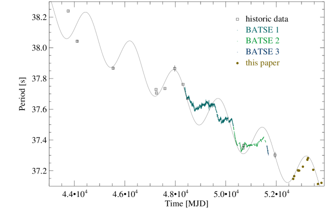
Figure 6: Long-term period evolution of OAO 1657$-$415. The historic data from the literature (see Table 2) were corrected for binary motion. The BATSE data are from public archive (1,3) and private communication by Mark Finger (2). The sinusoid with a period of 4.8 yr, superposed on a linear long-term spin-up, is to guide the eye to emphasise a quasi-periodic behaviour.

The complete set of data in Fig. 6 is described by a mean spin-up rate of $\dot{P}_{\mathrm{mean}}=-1.24\times 10^{-9}$ s s^-1. On top of this long-term mean spin-up deviations are observed with episodes of strong relative ($\dot{P}-\dot{P}_{\mathrm{mean}}$) spin-up and spin-down. In some of the spin-down episodes even the absolute spin-down $\dot{P}$ is quite strong (as in the first half of our measurements around MJD 53 000). The appearance in time of the deviations is suggestive of a quasi-periodic behaviour. We do not claim a formal value for the period, but show in Fig. 6 a model modulation by a sine curve with an amplitude of 0.13 s and a period of 1750 d (4.8 yr), which reproduces the main features of the long-term evolution. One could consider this period as the characteristical time for a typical spin-down/spin-up cycle.

3.4 Binary ephemeris

After having used the binary ephemeris of Chakrabarty et al. (1993) and Bildsten et al. (1997) for the pulse period analysis (as discussed in Section 3.2), we have analysed the non-binary-corrected light curve data from the INTEGRAL GPS in order to establish our own local ephemeris. We again made use of “running mean pulse profiles” (from sets of in general eight SCWs, the start of each set shifted by one SCW as compared to the previous one) and the phase connection techniques. For each of the 11 observation groups (see Table 1) a local ephemeris was established, which – except for observation 2 – are generally not very accurate because the observations are short and the intrinsic pulse period shows a strong variation with time (see above). Observation 2, however, samples about 2.5 binary cycles reasonably densely, such that a fit of the pulse arrival time delays (Fig. 7) can be performed and an ephemeris established. We find (keeping the orbital elements as before): $T_{90}=$ MJD $52\,663.893(10)$. Adding all other observations to the analysis yields the same result (with increased uncertainty).

Figure 7: Observed pulse delay times for the second observation period, which covers about 2.5 orbital cycles. The solid line shows the best fit for the orbital parameters (see Sect. 3.4). The residuals (observed $-$ calculated, lower panel) show some variation that may well be due to real pulse period variations on time scales shorter than one orbital period.

There is no indication for a secular change of the orbital period. Assuming $\dot{P}_{\mathrm{orb}}=0$, we can combine our new ephemeris with values from the past to arrive at a new sidereal period. Using, e.g., the $T_{90}$ of Chakrabarty et al. (1993) of MJD 48 515.99(5), and dividing the time difference to our ephemeris by 397 orbital cycles, we arrive at $P_{\mathrm{sid}}=P_{\mathrm{orb}}=10\aas@@fstack{d}448\,12\pm 0\aas@@fstack{d}000\,13$. Our $P_{\mathrm{orb}}$ is consistent with the value of Bildsten et al. (1997) within our uncertainty, which is reduced by a factor of 2.5 in comparison to that of Bildsten et al. (1997). Table 3 shows the current best set of orbital parameters.

We have done the same for the observed times of mid-eclipse: if the elapsed time between our mid-eclipse (MJD 52 663.64(5), see above) and that of Chakrabarty et al. (1993) (their Table 1: MJD 48 515.897(72)) is divided by 397 cycles we find $P_{\mathrm{ecl}}=10\aas@@fstack{d}447\,7\pm 0\aas@@fstack{d}000\,3$. The period found from eclipse timing is consistent (within uncertainties) with that found using the orbital ephemeris determined from pulse timing analysis. We point out that this need not be the case: with the finite eccentricity of $e=0.104$ apsidal motion is expected, and $P_{\mathrm{ecl}}$ is only equal to $P_{\mathrm{orb}}$ if $P_{\mathrm{ecl}}$ is found from averaging over one (or more) complete apsidal period(s) (see e.g. Deeter et al. 1987). But so far, the apsidal period of OAO 1657$-$415 is not known.

For the time covered by the INTEGRAL GPS observations we find that the centre of eclipse is earlier than our $T_{90}$ by $\Delta T=0\aas@@fstack{d}25\pm 0\aas@@fstack{d}05$. Using the values in Table 1 of Chakrabarty et al. (1993) we estimate that also in 1991/92 the eclipse was earlier than $T_{90}$ by $\Delta T=0\aas@@fstack{d}1\pm 0\aas@@fstack{d}05$. In principle, such observed time differences $\Delta T$ can be used to find the longitude of periastron. To first order $\Delta T=T_{\mathrm{ecl}}-T_{90}=-(P_{\mathrm{orb}}/\pi)\leavevmode\nobreak\ e\cos\omega$ (Deeter et al., 1987), where $\omega$ is the longitude of periapsis and $e$ the eccentricity. From the change of $\omega$ the rate of apsidal advance (and the apsidal period) can be found. Unfortunately, neither the data of Chakrabarty et al. (1993) nor our own data are accurate enough to yield a meaningful constraint.

Table 3: Current best set of orbital parameters: $T_{90}$ and period as estimated in this work, $a\sin\leavevmode\nobreak\ i$, eccentricity and $\omega$ taken from Bildsten et al. (1997).

Parameter	Value		Unit
Epoch ($T_{90}$)	52663.	893(10)	MJD
Period	10.	44812(13)	d
$a\sin\leavevmode\nobreak\ i$	106.	0(5)	lt-sec
eccentricity	0.	104(5)
$\omega$	93(5)		deg

Figure 8: Energy-resolved pulse profiles. The relative intensity scale is normalised to the average count rate level (horizontal dashed line) in the corresponding energy interval. The percentage values indicate the pulsed fraction. The pulsed fraction of the highest energy interval was set to 100%, as the negative minimum flux values were set to zero. The top panel shows the hardness ratio (see text). The vertical dashed lines denote the four phase intervals for which spectra were extracted. The pulse phase limits of the four intervals are: $\mathrm{a}=0.025-0.250$, $\mathrm{b}=0.25-0.50$, $\mathrm{c}=0.50-0.75$ and $\mathrm{d}=0.750-1.025$.

Figure 9: Variation of the pulsed fraction with energy. Horizontal bars denote the energy range for which the pulsed fraction was calculated.

3.5 Energy-resolved pulse profiles

With the above determined pulse periods, pulse profiles in seven different energy intervals (covering the range $20-160$ keV) of 720 SCWs were produced and superposed (using the sharp rise of the main pulse as phase reference - we call this pulse phase 0). The final energy-resolved pulse profiles are displayed in Fig. 8. The pulsation is clearly detected up to the highest energy range ($120-160$ keV).

The profiles consist of at least three components, the amplitudes of which decrease during the course of the pulse. For easier comparison the profiles for the different energy intervals are shown in the same relative scale (except for the energy range $120-160$ keV, where the plot needs a different scale due to the higher pulsed fraction and the larger errors). The pulsed fraction – indicated as percentage in Fig. 8 – increases linearly with energy in the range $30-70$ keV (Fig. 9). We calculated the pulsed fraction from the minimum and maximum flux values in the corresponding energy interval as $f_{\mathrm{pulsed}}=(F_{\mathrm{max}}-F_{\mathrm{min}})/(F_{\mathrm{max}}+F_{\mathrm{min}})$. This is – at least in the case of sinusoidal pulse profiles – equivalent to the standard definition $f_{\mathrm{pulsed}}=F_{\mathrm{pulsed}}/(F_{\mathrm{pulsed}}+F_{\mathrm{constant}})$, calculated from the values of the pulsed and the constant flux parts. It should be noted that negative $F_{\mathrm{min}}$ values were set to zero to avoid calculated pulsed fractions larger than 100%, which is the case for the highest energy interval shown in Fig. 8.

Also obvious from the plot is that the first maximum becomes asymmetric at higher energies, which indicates a harder spectrum in phase interval a (defined in Fig. 8). The top panel of Fig. 8 shows the hardness ratio calculated as ratio of the photon fluxes in the $40-160$ keV band to those in the $20-40$ keV band.

4 Spectral modelling

4.1 Introduction

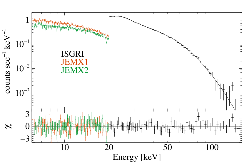
Figure 10: Phase-averaged broadband spectrum for ISGRI, JEM-X1, JEM-X2. The fitted model was HIGHECUT. To avoid artefacts in the residuals of the fit, the transition to the high energy cutoff was smoothed with an additional Gaussian absorption. The fit parameters are given in Table 4.

Table 4: Table of fit parameters for the phase-averaged broad band spectrum shown in Fig. 10 for two different spectral models (see text). A systematic error of 2% was assumed. The uncertainties given are at 90% confidence level for single parameter errors ($\chi^{2}_{\mathrm{min}}+2.7$).

Compon.	Parameter	Unit	Model A	Model B	Ref. a	Ref. b	Ref. c	Ref. d	Ref. e
phabs	$N_{\mathrm{H}}$ (JEM-X1, ISGRI)	$10^{22}$ cm-2		$0$ (frozen)	1.29	14.1	41	12.7	7.2
phabs	$N_{\mathrm{H}}$ (JEM-X2)	$10^{22}$ cm-2		$18.4^{+3.7}_{-3.6}$
powerlaw	$\Gamma$ (JEM-X2, ISGRI)		$1$ (frozen)	$1.27{\pm 0.05}$	1.07		1.0	0.83	0.60
powerlaw	$\Gamma$ (JEM-X1)		$1.3$ (frozen)	$1.27{\pm 0.05}$
powerlaw	normalisation (1 keV)	(keV cm2 s)-1	$0.055^{+0.003}_{-0.002}$	$0.12{\pm 0.02}$	0.06		0.046
highecut	Cutoff energy	keV	$21.6^{+1.0}_{-1.4}$	$24.4{\pm 0.9}$	12.82			13.0	$<$5.0
highecut	Folding energy	keV	$19.0{\pm 0.2}$	$21.2{\pm 0.5}$	29.37			21.2	17.0
gaussian	Fe line centre	keV			6.65	6.4 / 7.1	6.4	6.47	6.60
gaussian	Fe line width $(\sigma)$	keV			0.40	0.2 / 0.3	0.044	0.42	0.24
gaussian	Total flux in Fe line	$10^{-3}$ (cm2 s)-1			2.77	0.74 / 0.25	0.8		3.0
energy range		keV	6–160	6–160	3–100	0.5–10	4–8	1–100	3–40
red. $\chi^{2}$			1.00	0.94
DOF			258	253

^a Baykal (2000); ^b Audley et al. (2006), non eclipse spectrum, 2 Fe lines; ^c Chakrabarty et al. (2002); ^d Orlandini et al. (1999); ^e Kamata et al. (1990)

Due to calibration uncertainties below 20 keV and low flux above 160 keV the useable range of the ISGRI spectra was $20-160$ keV. The JEM-X spectra were used in the $6-20$ keV range, which we consider as the most reliable range. All spectra are background subtracted.

We used the following components for our spectral models: An absorbed power law model ($\exp[-\sigma(E)N_{\mathrm{H}}]E^{-\Gamma}$, XSPEC model phabs*powerlaw – in the following ABSPL), which influences only the JEM-X part of the spectra. The second component was an exponential cutoff power law model ($E^{-\Gamma}\exp[-E/E_{\mathrm{f}}]$, XSPEC model cutoffpl – in the following CUTOFFPL) or a power law with high energy cutoff ($E^{-\Gamma}\exp[-(E-E_{\mathrm{c}})/E_{\mathrm{f}}]$ if $E>E_{\mathrm{c}}$, else $E^{-\Gamma}$; XSPEC model powerlaw*highecut – in the following short HIGHECUT). These components are mainly determined by the ISGRI part of the spectra.

Being not able to fit the spectra with CUTOFFPL plus cyclotron absorption as described by Orlandini et al. (1999), we used in our analysis the HIGHECUT model (Model A in Table 4). In order to avoid artefacts in the residuals usually produced by the XSPEC highecut model at $E_{\mathrm{c}}$ (Kretschmar et al., 1997), the function was smoothed with a Gaussian absorption gabs as successfully exercised by Coburn et al. (2002). The centre of this Gaussian was set to $E_{\mathrm{c}}$ plus 1 keV (from experience with other spectra and confirmed by the fitting procedure). The width $\sigma$ and the depth $\tau$ of the Gaussian were found to be 2.2 keV and 0.9, respectively, and were subsequently fixed at these values.

The photon index $\Gamma$ for the ISGRI part of the phase-averaged spectra (Fig. 10) was fixed to unity, which is justified by the JEM-X2 part of the spectrum and is consistent with other spectral fits reported in literature (see Table 4). The JEM-X1 spectra show a significantly different photon index of 1.3 (the errors for all $\Gamma$ values are 0.05). There are several possible explanations for this behaviour: First, the JEM-X1 spectra cover the orbital phases from 0.25 to 0.65, while the JEM-X2 spectra are mainly located in the phase intervals $0.1-0.25$ and $0.65-0.8$. Second, they originate from different time intervals: JEM-X2 from MJD $52\,671-52\,869$ and JEM-X1 from MJD $53\,232-53\,795$. A third possibility might be the existence of uncertainties in the spectral calibration of the two instruments.

This difference in the JEM-X spectra could also be well fitted by an additional photon absorption in the JEM-X2 spectra (ABSPL, see Sect. 4.1). Model B in Table 4 shows the parameters in this model, which is formally Model A multiplied by the XSPEC model phabs. The photon index $\Gamma$ was kept identical for all 3 spectral parts (ISGRI, JEM-X1, JEM-X2). No absorption was assumed for the ISGRI and JEM-X1 part, while for JEM-X2 cold matter absorption was fitted. The fit led to a $N_{\mathrm{H}}$ of $(18.4\pm 3.6)\times 10^{22}\mathrm{cm}^{-2}$, which is within the range of other literature values shown in Table 4. This finding could imply that the spectra near the eclipse are more absorbed than in the centre of the orbital profile. On the other hand it could also mean that at least part of the strong variability of OAO 1657$-$415 is due to variable absorption, which was higher during the JEM-X2 part of the observation.

4.2 Pulse-phase resolved spectroscopy

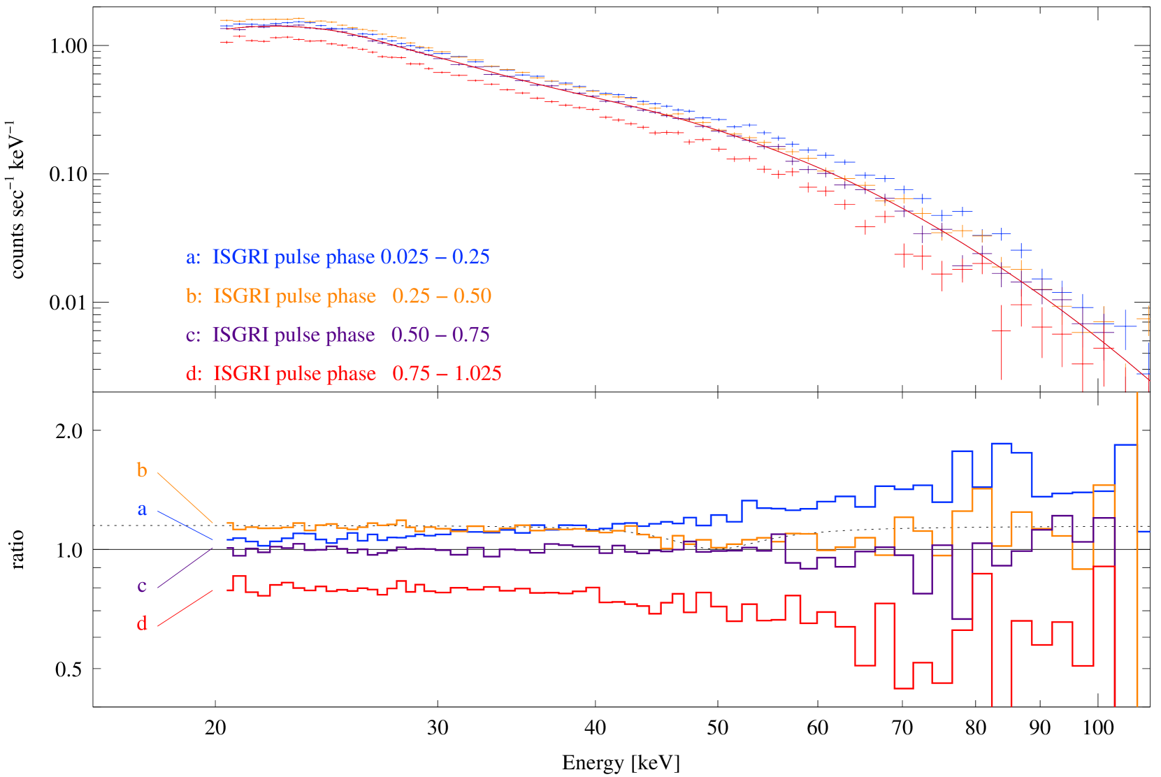
Figure 11: Phase-resolved ISGRI spectra for the four phase intervals as defined in Fig. 8. The solid line in the upper panel is the model fit of the phase-averaged spectrum as shown in Fig. 10 (model A of Table 4). To enhance the differences between the spectra of the four phase intervals the lower panel gives the ratios between the four spectra and the model of the phase-averaged spectrum in a logarithmic scale. The dotted line in the lower panel corresponds to a fit of spectrum b with a line feature at 49.3 keV.

We have investigated ISGRI spectra from the four pulse phase intervals indicated in Fig. 8. The spectra are shown in Fig. 11. We fitted all data using the HIGHECUT model, keeping the power law index fixed to $\Gamma=1.0$. The results are given in Table 5.

Table 5: Fit parameters for the spectral model HIGHECUT, Model A in Table 4. In the last line the fit parameters for the second phase interval are given for the same model, but multiplied by a cyclotron absorption^a. The uncertainties given are at 90% confidence level for single parameter errors ($\chi^{2}_{\mathrm{min}}+2.7$). No systematic errors were considered.

Phase		Red. $\chi^{2}$	DOF	$\Gamma$	Normalisation at 1 keV	Cutoff Energy	Folding Energy
					[$10^{-2}$ (keV cm2 s)-1]	[keV]	[keV]
0.025 –	0.25	0.99	68	1	6.1${}_{-0.3}^{+0.5}$	20.1${}_{-0.3}^{+0.6}$	21.4${}_{-0.3}^{+0.6}$
0.25 –	0.5	1.30	68	1	6.2${}_{-0.2}^{+0.4}$	22.0${}_{-0.3}^{+0.5}$	18.1${}_{-0.3}^{+0.5}$
0.5 –	0.75	1.02	68	1	5.4${}_{-0.2}^{+0.5}$	22.1${}_{-0.3}^{+0.6}$	18.7${}_{-0.3}^{+0.6}$
0.75 –	1.025	1.26	68	1	4.2${}_{-0.1}^{+0.2}$	23.2${}_{-0.3}^{+0.6}$	17.1${}_{-0.3}^{+0.6}$
0.25 –	0.5	1.03	68	1	6.4${}_{-0.2}^{+0.5}$	20.9${}_{-0.9}^{+1.9}$	19.1${}_{-0.3}^{+0.5}$

^a The cyclotron line parameters (XSPEC model cyclabs) were: energy 49.3 keV, width 5.4 keV, depth 0.136. These parameters were fixed after fitting them to a spectral range of $20-60$ keV, so that for the fit parameters shown in the last line also a DOF value of 68 is valid.

4.3 Search for cyclotron resonance scattering features

As cyclotron resonance scattering features are observed in several pulsars (see discussion in Sect. 5.2) we tried to find possible evidence of a cyclotron line feature. We therefore calculated the ratio of the spectra from the four phase intervals to the phase-averaged spectrum (model A of Table 4 with ISGRI parameters). In this way, differences between the individual spectra and features within these spectra are enhanced. The four individual spectra and the ratios are shown in Fig. 11. While spectrum c (pulse phase $0.5-0.75$) is nearly identical to the pulse-phase averaged spectrum (the ratio in the lower panel of Fig. 11 is around 1.0), spectrum a (phase $0.025-0.25$) is clearly harder and spectrum d (phase $0.75-1.025$) is clearly softer. Spectrum b (phase $0.25-0.5$) shows a slight “peculiarity”: there seem to be two components to the spectrum with a transition between 45 keV and 55 keV, or alternatively, a depression around these energies. Formally, a cyclotron line can be fitted with a centroid energy of 49.3 keV. The $\chi^{2}$ is reduced to 0.9 (DOF = 41) from 1.2 (DOF = 44), resulting in an F-Test value of 1 %, which is usually not considered as sufficient to state the detection of a cyclotron absorption line – also one should keep in mind that it is in general not correct to use an F-Test to test for the presence of a line (Protassov et al., 2002).

5 Summary and Discussion

5.1 The orbital profile

In the averaged light curve (Fig. 2) we found a dip at phase interval 0.55, which is confirmed by ASM measurements (Fig. 3) taken in the same time interval as the INTEGRAL observations, but homogeneously sampled. The dip is more pronounced in our INTEGRAL data, but we cannot exclude that this is an effect from the inhomogeneous sampling in the INTEGRAL data (see dashed line in both figures) with a minimum of measurements at the minimum of the profile. In order to evaluate the effects of the sampling we ran a statistical simulation, used to produce the “error bars” in Fig. 2. These bars show the range between the minimum and maximum values evaluated from 10 000 profiles calculated from 30 randomly chosen SCWs per phase bin. The dip around orbital phase 0.5 is always present, in line with the ASM results.

We note that the average profile should not be seen as a template for individual light curves, it rather seems to be the result of a random process. Some individual light curves have a maximum in the phase interval $0.2-0.5$, others (and more) have a maximum in the interval $0.6-0.85$. So the strong variability of the source may be weakly correlated with the orbital phase in such a way that the chance for a “low state” is quite high at phase 0.55.

The physical origin of this orbital modulation is still unclear. Topics to be discussed in this context should comprise absorption, scattering, a (partial) blockage of the line of sight to the neutron star, or variations of the accreted wind. All of these mechanisms will be subject to further investigations.

As the pulsar can be considered as a point source compared to its B supergiant companion, the slope of the ingress and egress indicates a soft transition from the stellar atmosphere to the stellar wind region with a decreasing optical thickness for the radiation emitted by the pulsar. The density profile of the outer regions of the supergiant was modelled by Bulik et al. (2005) with an exponential density distribution. They fitted the modelled absorption to the observed folded light curve, which was composed from 480 INTEGRAL SCWs. This model did not account for the asymmetric shape of the orbital profile and should be refined in a further analysis.

5.2 Timing analysis

The INTEGRAL observations extend the long-term monitoring of OAO 1657$-$415 and cover a period with a torque reversal from strong spin-down to strong spin-up. We have compiled all available pulse period measurements from the literature and, where necessary, converted the values to the intrinsic neutron star spin period. We find that the long-term spin-up is continued and determine a mean rate of $\dot{P}=-1.24\times 10^{-9}s\,s^{-1}$. The spin-down/spin-up behaviour observed by INTEGRAL, together with the historical data imply a quasi-periodic variation of the pulse period with a period of roughly 5 years, superimposed on the long-term mean spin-up.

The orbital elements were determined from pulse timing analysis. Combining our results with previous data we determine an orbital period with improved accuracy: $P_{\mathrm{orb}}=10\aas@@fstack{d}448\,12\pm 0\aas@@fstack{d}000\,13$. We find a difference between $T_{90}$ and the centre of eclipse of $(0\aas@@fstack{d}3\pm 0\aas@@fstack{d}1)$, which is consistent with the previously determined value, and does not allow a conclusion about a possible apsidal advance.

The long-term evolution of the spin period is similar to that of Her~X-1. In this object a quasi-periodic spin-up/down variation is found with a period of about 5 yr, (as in OAO 1657$-$415) superimposed on a long-term spin-up (Staubert et al., 2006). Since in Her X-1 the period variations are correlated with the 35 d turn-on behaviour and the quasi-periodically repeating anomalous low states, this phenomenon is generally connected to the precessing accretion disk and an associated variation in the mass accretion onto the neutron star.

In contrast to Her X-1, however, OAO 1657$-$415 is a high mass, wind accreting system and we have no direct evidence of an accretion disk. Also no correlation between flux and period change is observed (İnam & Baykal, 2000). So the conditions are probably different compared to the low mass X-ray binary Her X-1. OAO 1657$-$415 is probably better compared to other high mass X-ray binaries (HMXB), e.g. Cen~X-3 and Vela~X-1. The long-term frequency histories presented by Bildsten et al. (1997) for several pulsars, show a secular spin up for Cen X-3 with a weak quasi periodic modulation of about 5 to 8 years. For Vela X-1, on the other hand, a secular spin down is shown, but with a torque reversal around MJD 44 000 (spin up to spin down) and possibly also around MJD 49 000 (spin down to spin up). Between these dates also a quasi periodic characteristics of the period evolution with a period around 5 years might be inferred. We note here that these quasi-periodic pulse period variations, seen in several accreting X-ray pulsars, have not found much attention in the literature.

In addition to the long-term quasi-periodicity we have found variations of the pulsar period on time scales shorter than the orbital period (residuals in Fig. 7). Bildsten et al. (1997) have discussed power spectra of torque fluctuations for several objects, including OAO 1657$-$415. While Her X-1 and Vela X-1 showed a white noise power density spectrum, Cen X-3 shows red noise. For OAO 1657$-$415 Bildsten et al. (1997) also noted a red noise spectrum. But a closer look at the power density spectrum shows a slight increase in power density for frequencies above the orbital frequency of about $1\times 10^{-6}$ Hz. OAO 1657$-$415 has the highest power density at high frequencies of all pulsars presented in Bildsten et al. (1997), which is consistent with our finding of pulse period changes on time scales much shorter the orbital period. Also Blondin et al. (1990) expect fluctuations in the spin-up/spin-down on short time scales as a result of changes in the sign and magnitude of the accretion torque.

5.3 The pulse profile

The energy-resolved pulse profiles show a complex structure with one main peak followed by at least two somewhat weaker peaks. The spectrum of the rising part of the main peak is clearly harder than in the other parts of the pulse.

The change of spectral hardness with pulse phase is commonly observed. Below 10 keV this behaviour might be modelled by a variation of an absorbing column density $N_{\mathrm{H}}$ (e.g. Cen X-3, Santangelo et al., 1999a) but for energies above $10-20$ keV cold absorption plays no role anymore. A mixture of different emission regions, as proposed by Kraus et al. (1996) to explain energy-resolved pulse profiles of Cen X-3, might explain the observed profiles, but such detailed theoretical modelling is beyond the scope of this paper.

As in many other accreting pulsars, e.g. 4U~0115+63 (Tsygankov et al., 2007) or GX 1+4 (Ferrigno et al., 2007), the pulsed fraction increases with energy. Tsygankov et al. (2007) point out that in the accretion column the region emitting harder photons is closer to the neutron star surface and therefore can be more obscured during certain pulse phases than the region higher up emitting photons of lower energy.

5.4 Spectral analysis

The broad band spectrum, composed from ISGRI and JEM-X spectra could be modelled by the HIGHECUT model. We could not find an indication for a cyclotron absorption in the phase-averaged spectrum.

Blondin et al. (1990) have done hydrodynamic simulations of the accretion by a neutron star from stellar wind in massive X-ray binaries. Their work points to episodic changes of the mass accretion rate, which results in corresponding changes of the X-ray luminosity on a time scale of hours. They also find a variation of integrated column density, which varies with orbital phase in such a way that it is highest near eclipse and lowest at orbital phase 0.5. This is in good agreement with our findings for the JEM-X1 and JEM-X2 spectra, which show a higher absorption near eclipse.

Phase-resolved spectra were produced from ISGRI observations for 4 phase intervals. These spectra show significant differences. Phase $0.025-0.25$, covering the rising part of the main pulse peak, shows the hardest spectrum, while phase $0.75-1.025$ has the softest spectrum. Phase $0.5-0.75$ fits nearly exactly the phase-averaged spectrum, while phase $0.25-0.5$ shows a feature at about 50 keV, which is reminiscent of a cyclotron absorption line, but with a significance too weak to prove its existence.

Apart from not being able to detect a cyclotron line in our data, it would not be unlikely to find such a line in the spectrum of phase interval $0.25-0.5$, as it is common to several pulsars that cyclotron lines are visible only – or at least most prominent – in the falling part of the main pulse, e.g. 4U 0115+63 (Santangelo et al., 1999b), GX~301-2 (Kreykenbohm et al., 2004), Cen X-3 (Burderi et al., 2001), Vela X-1 (Kreykenbohm et al., 2002) and possibly also GX 1+4, which shows a likewise weak absorption feature at 34 keV (Ferrigno et al., 2007).

6 Conclusions

We have presented a spectral and timing analysis of INTEGRAL observations of OAO 1657$-$415, which span a time range of about 3.5 years. Though we found our results to be compatible with similar observations of other high mass X-ray binaries, we state that a consistent model for OAO 1657$-$415 is still missing. Such a model should explain the nature of the strong variability and its possibly weak correlation with the orbital phase. Also the origin of the fluctuations of the pulse period with its observed long-term quasi periodic behaviour should be addressed by this model. Detailed analysis is also required to explain the rather complex structure of the pulse profiles. Further observations with continuous coverage of OAO 1657$-$415 would be required to settle the question of a potential spectral feature in the falling part of the main peak of the pulse profile.